Making Maps from Planck LFI 30GHz Data with Asymmetric Beams and Cooler Noise

The Planck satellite will observe the full sky at nine frequencies from 30 to 857 GHz. Temperature and polarization frequency maps made from these observations are prime deliverables of the Planck mission. The goal of this paper is to examine the effects of four realistic instrument systematics in the 30 GHz frequency maps: non-axially-symmetric beams, sample integration, sorption cooler noise, and pointing errors. We simulated one year long observations of four 30 GHz detectors. The simulated timestreams contained cosmic microwave background (CMB) signal, foreground components (both galactic and extra-galactic), instrument noise (correlated and white), and the four instrument systematic effects. We made maps from the timelines and examined the magnitudes of the systematics effects in the maps and their angular power spectra. We also compared the maps of different mapmaking codes to see how they performed. We used five mapmaking codes (two destripers and three optimal codes). None of our mapmaking codes makes an attempt to deconvolve the beam from its output map. Therefore all our maps had similar smoothing due to beams and sample integration. This is a complicated smoothing, because every map pixel has its own effective beam. Temperature to polarization cross-coupling due to beam mismatch causes a detectable bias in the TE spectrum of the CMB map. The effects of cooler noise and pointing errors did not appear to be major concerns for the 30 GHz channel. The only essential difference found so far between mapmaking codes that affects accuracy (in terms of residual root-mean-square) is baseline length. All optimal codes give essentially indistinguishable results. A destriper gives the same result as the optimal codes when the baseline is set short enough (Madam). For longer baselines destripers (Springtide and Madam) require less computing resources but deliver a noisier map.

1 Introduction

Starting in 2003, Planck Working Group 3 (the “CTP” group) undertook a comparison of mapmaking codes in increasingly realistic situations. The approach to realism proceeded in four steps, named after the locations of working meetings of the group (Cambridge, Helsinki, Paris, and Trieste). Results from the Cambridge, Helsinki, and Paris steps have been presented in previous papers (Poutanen et al. Pou06 (2006), Ashdown et al. 2007a , 2007b ). Here we present results from the Trieste simulations, designed to determine how mapmaking codes handled four aspects of real Planck data not included in previous simulations. The first was non-axially-symmetric beams. In previous simulations, we assumed that the beams on the sky were axially symmetric Gaussians. The second was the effect of detector sample integration, which introduces an effective smearing of the sky signal along the scanning direction. The third was “cooler noise”, representing the effect of temperature fluctuations induced in the focal plane by the 20 K sorption cooler. The fourth was the pointing errors. In previous simulations, we assumed that the detector pointings were known without error in the mapmaking. In this paper we present the results of this latest round of simulations, which are realistic enough to allow us to draw some preliminary conclusions about mapmaking. We also outline additional work that must be done before final conclusions can be drawn.

The organization of the paper is as follows. In Section 2 we describe the simulations that produced the time-ordered data (TOD) streams that were inputs to our mapmaking. In Section 3 we give the inputs that were used in these simulations. In Section 4 we describe the mapmaking codes we used in this study. Section 4 details the changes that we made in those codes since our earlier Paris simulation round. Section 5 gives the results of our Trieste simulation round and the computational resource requirements of our mapmaking codes are listed in Section 6. Finally we give our conclusions and proposal for future mapmaking tests in Section 7. In Appendix A we describe an analytic model that we used in explaining the effects of beam mismatch in the CMB maps. Appendix A also shows how we can use this model to correct these effects from the observed spectrum.

2 Simulations

We used the Level-S simulations pipeline (Reinecke at al. Rei06 (2006)) to generate 1-year intervals of simulated detector observations (time-ordered data streams, or TODs). As in the Paris round (Ashdown et al. 2007b ) all simulations were done at 30 GHz, the lowest Planck frequency. This was chosen, because the TOD and maps are the smallest in data size for this frequency, minimizing the computer resources required for the simulations, and because the beams are furthest from circular, emphasizing one of the effects we are trying to study. We simulated the relevant sky emissions (CMB, dipole, diffuse galactic foreground emissions, and the strongest extragalactic point sources) in both temperature and polarization, plus a number of instrumental effects: uncorrelated (white) noise, correlated ($1/f$) noise, noise from sorption cooler temperature fluctuations, both circular and elliptical detector beams, sample integration, semi-realistic nutation of the satellite spin axis, and fluctuations of the satellite spin rate.

TODs 366 days long were generated for the four 30 GHz LFI detectors (Low Frequency Instrument), with $1.028\times 10^{9}$ samples per detector corresponding to a sampling frequency of $f_{\mathrm{s}}=32.5$ Hz.

For every sky component we made four different simulated TODs. A TOD included the effects of either axially symmetric or asymmetric Gaussian beams and the sample integration was either on or off. We call these four TODs as

• Symmetric beams & no sampling

• Symmetric beams & sampling

• Asymmetric beams & no sampling

• Asymmetric beams & sampling.

For the instrument noise (uncorrelated + correlated) we used the noise TODs of the Paris round (Ashdown et al. 2007b ). Finally, we had a TOD of the cooler noise. Maps were later made from different combinations of these TODs.

3 Inputs

3.1 Scanning strategy

The correspondence between the sample sequence of the TOD and locations on the sky is determined by the scan strategy. The Planck satellite will orbit the second Lagrangian point ($L_{2}$) of the Earth-Sun system (Dupac & Tauber Dup05 (2005)), where it will stay near the ecliptic plane and the Sun-Earth line.

Planck will spin at $\sim 1$ rpm on an axis pointed near the Sun-Earth line. The angle between the spin axis and the optical axis of the telescope (telescope line-of-sight, see Fig. 2) is $85\degr$; the detectors will scan nearly great circles on the sky. The spin axis follows a circular path around the anti-Sun direction with a period of six months; the angle between the spin axis and the anti-Sun direction is 7 .^∘5. The spin axis thus follows a cycloidal path across the sky, (like the one we used in our Paris round, Ashdown et al. (2007b )). In this simulation the spin axis is repointed hourly. During each repointing the projection of the spin axis onto the ecliptic moves by a fixed 2.^′5. Our simulation had 8784 repointings in total. We assumed non-ideal satellite motion, with spin axis nutation and variations in the satellite spin rate.

The scan strategy planned for flight differs from the one used here only in that instead of repointing once per hour with a fixed offset in ecliptic longitude, we will repoint in 2^′ intervals along the cycloid. To maintain the 2.^′5 hr^-1 average rate of motion along the ecliptic, the time spent at a given spin axis pointing will vary somewhat.

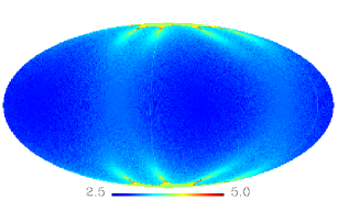
Figure 1: Number of hits per pixel ($n_{\mathrm{hit}}$) for the scan strategy applied in this study. The hit map is shown in the ecliptic (left) and galactic (right) coordinates. The latter map shows the areas of the ecliptic poles more clearly. Both maps include the hits of all four LFI 30 GHz detectors. The scale is $\log_{10}(n_{\rm{hit}})$.

Spin rate variations were chosen randomly at every repointing from a truncated Gaussian probability distribution with parameters (0 .^∘1 s^-1 RMS, 0 .^∘3 s^-1 max). The abbreviation “RMS” refers to the root-mean-square.

The satellite spin axis nutated continuously according to the satellite dynamics. The nutation amplitude was chosen randomly at every repointing to mimic the disturbance that the repointing maneuver causes in the spin axis motion. In this simulation the Gaussian distribution of nutation amplitudes ranged from $0\hbox{\hbox to0.0pt{.\hss}\kern 0.80002pt}^{\scriptscriptstyle\prime}\hbox{\kern-0.29999pt}006$ to $16\hbox{\hbox to0.0pt{.\hss}\kern 0.80002pt}^{\scriptscriptstyle\prime}\hbox{\kern-0.29999pt}4$, with mean and standard deviation values of $1\hbox{\hbox to0.0pt{.\hss}\kern 0.80002pt}^{\scriptscriptstyle\prime}\hbox{\kern-0.29999pt}2$ and $0\hbox{\hbox to0.0pt{.\hss}\kern 0.80002pt}^{\scriptscriptstyle\prime}\hbox{\kern-0.29999pt}8$. The nutation amplitudes of the repointings were all $\leq 3\hbox{\hbox to0.0pt{.\hss}\kern 0.80002pt}^{\scriptscriptstyle\prime}\hbox{\kern-0.29999pt}2$ except for two large excursions (out of 8784) of $4\hbox{\hbox to0.0pt{.\hss}\kern 0.80002pt}^{\scriptscriptstyle\prime}\hbox{\kern-0.29999pt}3$ and $16\hbox{\hbox to0.0pt{.\hss}\kern 0.80002pt}^{\scriptscriptstyle\prime}\hbox{\kern-0.29999pt}4$. This level of nutation is many times larger than is (now) expected in flight.

The discussion of the performance of the Planck pointing system is outside the scope of this paper. Our simulation of pointing is based on the results of a detailed simulation of the spacecraft pointing dynamics. In the simulations of this paper the satellite attitude (“satellite pointing”) was sampled at 1 Hz. In flight the Planck attitude will be sampled at a higher rate.

We used the HEALPix pixelisation scheme (Górski et al. 2005a ) with $N_{\rm side}=512$. A map of the full sky contains $12N_{\rm side}^{2}$ pixels. The Stokes parameters Q and U at a point on the sky are defined in a reference coordinate system ($\mathbf{e}_{\theta},\mathbf{e}_{\varphi},\mathbf{n}$), where the unit vector $\mathbf{e}_{\theta}$ is along the increasing $\theta$ direction, $\mathbf{e}_{\varphi}$ is along the increasing $\varphi$ direction, and $\mathbf{n}$ points to the sky (Górski et al. 2005b ). The angles $\theta$ and $\varphi$ are the polar and azimuth angles of the spherical polar coordinate system used for the celestial sphere.

The number of hits per pixel from all detectors is shown in Fig. 1. At this resolution every pixel was hit.

3.2 Telescope beams

The horns of the LFI detectors sit in the Planck telescope focalplane (Fig. 2). The center of the field of view, which is empty in the figure, is populated with the beams of the HFI bolometers (High Frequency Instrument). There are two 30 GHz horns in the focalplane. The corresponding beams are labelled with “27” and “28” in Fig. 2. Behind each horn we have two detectors tuned to orthogonal linear polarizations, called LFI-27a, LFI-27b, LFI-28a, and LFI-28b. For simplicity, we refer hereafter the field of view as focalplane.

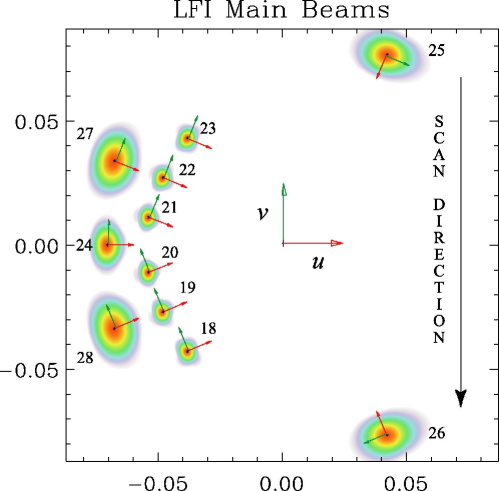
Figure 2: Footprint of the Planck LFI focalplane on the sky as seen by an observer looking towards the satellite along its optical axis. The origin of a right-handed $uv$-coordinate system is at the center of the focalplane (telescope line-of-sight). The $z$-axis is along the line-of-sight and points towards the observer. Labels “18–23” refer to 70 GHz horns, “24–26” refer to 44 GHz horns, and “27–28” refer to 30 GHz horns. Each beam has its own coordinate system as shown in the figure. The coordinate axes show the polarization orientations for the co–polar beams of the “a” and “b” radiometers. The focalplane scans the sky as the satellite spins. The scanning direction is indicated by an arrow. The $+u$ axis points to the spin axis of the satellite. The centers of the 30 GHz beams sweep $\backsim$$1\degr$ from the ecliptic poles when the spin axis is in the ecliptic plane. In Appendix A we need the angle from the scan direction to the $u$-axis of horn “27”. This angle is 67 .^∘5.

The time-ordered data were simulated using two sets of beams. The first set were circular Gaussian beams of the same beamwidth for all of the detectors. The second set were the best-fit elliptical beams for the LFI 30 GHz detectors. The beam parameters that we used in our simulations, are given in Table 1. These were obtained by fitting a bivariate Gaussian to the co–polar component of each beam over the whole angular area in which each beam was calculated. For the 30 GHz beams this was $-0.026<$ $u$,$v$ $<0.026$.

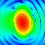
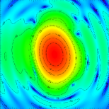
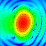
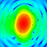
Figure 3: Contour plot in the $uv$-plane ($-0.026<$ $u$,$v$ $<0.026$) of the main beam co-polar component computed for the 30 GHz feed horns, assuming an ideal telescope. The color scale goes from -90 to 0 dB. The fit bivariate Gaussian contours are superimposed with dotted lines. From left to right the beams are for LFI-27a/b and LFI-28a/b. They are perfectly symmetric beams with respect to the $u$-axis because of the symmetry of the Planck LFI optics.

TABLE 1

Beams

Detector       FWHM^a Ellipticity^b $$\psi_{\rm pol}^{c} \psi_{\rm ell}^{d} \phi_{\rm uv}^{e} \theta_{\rm uv}^{e} \psi_{\rm uv}^{e} 32\hbox{\hbox to0.0pt{.\hss}\kern 0.80002pt}^{\scriptscriptstyle\prime}\hbox{\kern-0.29999pt}1865 \ldots - 32\hbox{\hbox to0.0pt{.\hss}\kern 0.80002pt}^{\scriptscriptstyle\prime}\hbox{\kern-0.29999pt}1865 \ldots - 32\hbox{\hbox to0.0pt{.\hss}\kern 0.80002pt}^{\scriptscriptstyle\prime}\hbox{\kern-0.29999pt}1865 - \ldots - 32\hbox{\hbox to0.0pt{.\hss}\kern 0.80002pt}^{\scriptscriptstyle\prime}\hbox{\kern-0.29999pt}1865 - \ldots - 32\hbox{\hbox to0.0pt{.\hss}\kern 0.80002pt}^{\scriptscriptstyle\prime}\hbox{\kern-0.29999pt}2352 - 32\hbox{\hbox to0.0pt{.\hss}\kern 0.80002pt}^{\scriptscriptstyle\prime}\hbox{\kern-0.29999pt}1377 - 32\hbox{\hbox to0.0pt{.\hss}\kern 0.80002pt}^{\scriptscriptstyle\prime}\hbox{\kern-0.29999pt}2352 - - 32\hbox{\hbox to0.0pt{.\hss}\kern 0.80002pt}^{\scriptscriptstyle\prime}\hbox{\kern-0.29999pt}1377 - -$$ Symmetric 27a.        1.0 0 .^∘2 153 .^∘6074 4 .^∘3466 22 .^∘5 27b.        1.0 89 .^∘9 153 .^∘6074 4 .^∘3466 22 .^∘5 28a.        1.0 0 .^∘2 153 .^∘6074 4 .^∘3466 22 .^∘5 28b.        1.0 89 .^∘9 153 .^∘6074 4 .^∘3466 22 .^∘5 Asymmetric 27a.        1.3562 0 .^∘2 101 .^∘68 153 .^∘6074 4 .^∘3466 22 .^∘5 27b.        1.3929 89 .^∘9 100 .^∘89 153 .^∘6074 4 .^∘3466 22 .^∘5 28a.        1.3562 0 .^∘2 78 .^∘32 153 .^∘6074 4 .^∘3466 22 .^∘5 28b.        1.3929 89 .^∘9 79 .^∘11 153 .^∘6074 4 .^∘3466 22 .^∘5

^aGeometric mean of full width at half maximum (FWHM) of the major and minor axes of the beam ellipse. Symmetric beam FWHM was chosen to be the arithmetic mean of the two FWHMs of the asymmetric beams. In practice the beamwidths will not be known to this level of precision, but we give additional significant figures here to show the level of variation of the widths, and to reflect what was actually used in the simulations.

^bRatio of the FWHMs of major and minor axes.

^cAngle between $$u$$-axis and polarization sensitive direction (see Fig. 2).

^dAngle between $$u$$-axis and beam major axis (see Fig. 2). This angle is irrelevant for axially symmetric beams.

^eAngles giving the position of the detectors in the focalplane. They give the rotation of the detector $$uvz uvz$$-coordinate system from its initial pointing and orientation (aligned with the telescope line-of-sight -axes) to its actual pointing and orientation in the focalplane (see Fig. 2).

Realistic main beams have been simulated in the co- and x-polar basis according to the Ludwig’s third definition (Ludwig Ludwig (1973)) in $uv$-spherical grids with 301 $\times$ 301 points ($\Delta u=\Delta v\simeq 10^{-4}$). Each main beam (Fig. 3) has been computed in its own coordinate system in which the power peak falls in the center of the $uv$-grid and the major axis of the polarization ellipse is along the $u$-axis. In this condition, a well defined minimum appears in the x-polar component in correspondence to the maximum of the co-polar component.

Main beam simulations have been performed using the physical optics considering the design telescope geometry and nominal horn location and orientation on the focalplane as described in Sandri et al. (San04 (2004)). The computation was carried out with GRASP8, a software developed by TICRA (Copenhagen, Denmark) for analysing general reflector antennas. The field of the source (feed horn) has been propagated on the subreflector to compute the current distribution on the surface. These currents have been used for evaluating the radiated field from the sub reflector. The calculation of the currents close to the edge of the scatterer has been modeled by the physical theory of diffraction. The radiated field from the sub reflector has been propagated on the main reflector and the current distribution on its surface is used to compute the final radiated field in the far field.

In this paper we considered the effects of the co-polar main beams only and did not include the effects of the x-polar beams in our simulations. In making maps from data with both circular and elliptical beams, we can quantify the effect of the elliptical beams in the maps and in the power spectra derived from the maps.

3.3 Signal sampling and integration

The readout electronics of the LFI 30 GHz channel sample the signal measured by the detectors at 32.5 Hz. The value recorded in each sample is the average of the measured signal over the period since the last sample. This non-zero integration time has the effect of widening of the beam along the scan direction. If the spin speed remains constant throughout the mission, this effect cannot be separated from the shape of the beam.

To quantify this effect, the TOD have been simulated using two options for the sampling. The first is to use instantaneous sampling, where the signal is not integrated over the past sample period, rather the sample value is given by the sky signal at the instant the sample is recorded. This option gives an idealized result to compare to the realistic sampling behaviour.

In the second and realistic option, there is an additional effect which must be taken into account. In the Level-S simulation pipeline, the pointing of the detector is sampled at the same rate as the signal from the detector and given at the instants the samples are taken. However, the effect of the integration time is to smear the sample over the past sample period; in effect, the reported pointing lags the signal by half a sample period. In order to minimise the residuals in the mapmaking, some of the codes used to produce the results in this paper can perform an interpolation to shift the pointing back by half of a sample period to the middle of the sample.

3.4 Noise

3.4.1 Detector noise

We used the instrument noise from our Paris round of simulations (Ashdown et al. 2007b ). Its uncorrelated (white) noise was simulated at the level specified in the detector database. Its nominal standard deviation per sample time was $\sigma$ = 1350 $\mu$K (thermodynamic (CMB) scale). Correlated $1/f$ noise was simulated from a power spectrum with a knee frequency of 50 mHz and slope $-1.7$. For the details of the noise generation see Ashdown et al. 2007b . Subsequent tests of the 30 GHz flight detectors show a lower knee frequency than 50 mHz, so these simulations can be taken as providing a conservative upper limit on $1/f$ noise. No correlation was assumed between the noise TODs of different detectors. For the optimal and Madam mapmaking codes, perfect knowledge of the noise parameter values was assumed in the mapmaking phase.

3.4.2 Sorption cooler temperature fluctuations

The Planck sorption cooler has two interfaces with the instruments, LVHX1 with HFI and LVHX2 with LFI (LVHX = Liquid-Vapor Heat eXchanger). The nominal temperature of LVHX1 is 18 K, providing precooling for the HFI 4-K cooler. The HFI 4-K cooler in turn cools the HFI housing and the LFI reference loads. The temperature of the HFI housing is stabilized by a Proportional-Integral-Differential (PID) control. LVHX2 determines the ambient temperature of the LFI front end. Its nominal temperature is 20 K.

Temperature fluctuations from the coolers affect the LFI data in three ways. First, fluctuations in LVHX2 propagate through the LFI structure to the LFI horns, resulting in fluctuations in additive thermal noise from the throats of the horns (where the emissivity is highest). Second, fluctuations in the LFI structure driven by LVHX2 propagate to HFI both by radiation and by conduction through struts supporting the HFI, and thence the LFI reference loads. Any temperature fluctuations of the reference loads will appear as spurious signals in the LFI detectors. A significant part of these fluctuations are suppressed by the HFI 4-K PID control, but the 30 GHz loads are between the struts and the control stage, so fluctuations are incompletely suppressed. Third, temperature fluctuations of the LFI reference loads are also driven by LVHX1, propagated indirectly through HFI. This last effect is quite small.

A coupled LFI/HFI thermal model was not available when the work reported in this paper was performed, so we were unable to include all of these effects realistically. Instead, in this paper we consider only the direct effect of LVHX2 instabilities on the feeds.

The propagation of LVHX2 temperature fluctuations to LFI output signals involves two transfer functions (TF):

• TF1 describes how the temperature fluctuations of the cold end propagate to the temperature fluctuations of the LFI front end.

• TF2 describes how the fluctuations of the ambient temperature of the LFI front end translate into a variation of the output signal of a detector.

The Planck LFI instrument team developed TF1 from the LFI thermal model. TF2 is described in Seiffert et al. (Sei02 (2002)). The thermal mass of the LFI front end suppresses fast temperature variations, so TF1 rolls off steeply at high frequencies. TF2 is a constant multiplier that is different for detectors of different frequency channels. The impact of the sorption cooler temperature fluctuations on the output signals of the LFI detectors has been discussed by Mennella et al. (Men02 (2002)).

For this study, simulated cooler TODs for the four LFI 30 GHz detectors were generated as follows. The LFI instrument team applied TF1 and TF2 to a $\backsim$100 hour sequence of LVHX2 cold end temperatures taken during cooler operation, producing a $\backsim$100 hour segment of data that approximates the fluctuations as they would appear at the output of an LFI 30 GHz detector. Three hours of these data from the beginning and end of the chunk are shown in Fig. 4. The cooler signal has a distinct periodicity, whose cycle time is $\backsim$760 s. Every sixth peak is stronger than the other peaks. Fig. 4 shows that the cycle time and the amplitude of the sorption cooler fluctuations remain stable over the $\backsim$100 hour period.

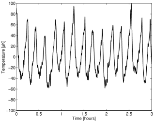
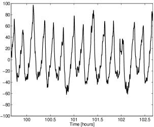
Figure 4: Variations of the output signal (TOD) of an LFI 30 GHz detector caused by the temperature fluctuations of the sorption cooler cold end. We show here the beginning (left) and the end (right) of a $\backsim$100 hour segment of data. The signal is a result of applying LFI thermal transfer functions to the cold end temperature data measured from the sorption cooler flight hardware. The thermal transfer functions were derived from the LFI thermal model developed by the Planck LFI instrument team. The vertical axis is antenna temperature in microkelvins at 30 GHz.

We used linear interpolation to increase the sampling rate of the cooler signal (Fig. 4) from its original 1 Hz to the detector sampling rate 32.5 Hz. After that we glued a number of these $\backsim$100 hour segments one after another to obtain a one year long cooler TOD. We used a $\backsim$10 hour overlap in the boundaries of the successive segments. The segments were manually adjusted in the time axis to give a good alignment of the fluctuation peaks and valleys in the overlap region. Finally we multiplied the end of a previous segment with linear weights descending from 1 to 0 and the beginning of the next segment with linearly ascending weights (ascending from 0 to 1) before summing the segments in the overlap region.

The resolution of the LFI thermal transfer function model could not distinguish between different detectors at 30 GHz at the time of this work. Therefore, in this paper all four LFI 30 GHz detectors were represented by the same one-year-long cooler TOD.

3.5 Dipole

The temperature Doppler shift arises from the (constant) motion of the solar system relative to the last scattering surface and from the satellite motion relative to the Sun. The latter signal is usually used for the calibration of the CMB observations. In this paper we assumed a perfect calibration and did not study the effects of calibration errors in our maps. We therefore chose to include the temperature Doppler shift of the solar system motion in our simulations, but we did not include the part that arises from the satellite motion relative to the Sun.

3.6 CMB

As in the Paris round (Ashdown et al. 2007b ), the CMB template used here is WMAP (Wilkinson Microwave Anisotropy Probe) constrained as described in the following, and included in the version 1.1 of the Planck reference sky. It is modelled in terms of the spherical harmonic coefficients, $a_{\ell m}^{T,E,B}$, where $T$ refers to temperature, and $E$ and $B$ refer to the polarization modes. The $a_{\ell m}^{T,E,B}$ were determined for multipoles up to $\ell=3000$.

For $\ell<70$, the $a_{\ell m}^{T}$ were obtained by running the anafast code of the HEALPix package on the first-year WMAP CMB template obtained by Gibbs sampling the data (Eriksen et al. Eri04 (2004)). The $a_{\ell m}^{E}$ were then given by

$$a_{\ell m}^{E}=a_{\ell m}^{T}\frac{C_{\ell}^{TE}}{C_{\ell}^{TT}}+\left(\frac{x_{\ell m}+iy_{\ell m}}{\sqrt{2}}\right)\sqrt{C_{\ell}^{EE}-\frac{C_{\ell}^{TE}}{C_{\ell}^{TT}}C_{\ell}^{TE}},$$ (1)

where $C_{\ell}^{XY}$ $(X,Y=T,E)$ is the best fit angular power spectrum to the WMAP data, and $x_{\ell m}$ and $y_{\ell m}$ are Gaussian distributed random variables with zero mean and unit variance. For $m=0$, the imaginary part of $y_{\ell m}$ and the $\sqrt{2}$ were not applied.

For $\ell>70$, we used the synfast code to generate the $a_{\ell m}^{T,E}$ as a random realization of the $C_{\ell}$ coefficients of the theoretical WMAP best fit cosmological model.

3.7 Foreground emission

With the exception of the Sunyaev-Zel’dovich (SZ) signal from clusters of galaxies, foregrounds have been modelled according to v1.1 of the Planck reference sky, as for the CMB case. In this section we describe how the various components have been modeled. SZ sources and extra-Galactic radio sources have been added since Ashdown et al. (2007b ).

3.7.1 Diffuse emission

We include synchrotron emission from free electrons spiraling around the Galactic magnetic field and bremsstrahlung emitted by electrons scattering onto hydrogen ions. We also include the emission from thermal dust grains; although subdominant with respect to the other components at intermediate and high Galactic latitudes, the brighest dusty emission regions across the Galactic plane are still relevant at 30 GHz. The total intensity information on these components is obtained from non-Planck frequencies, 408 MHz and 3000 GHz for synchrotron and dust, respectively, as well as $H\alpha$ regions tracing the bremsstrahlung. No comparable all-sky information exists for the linear polarization component. The latter has been simulated by exploiting data at low and intermediate latitudes in the radio and microwave bands (see Ashdown et al. 2007b for details).

3.7.2 Extra-galactic radio sources

Emission from unresolved extra-Galactic radio sources has been obtained from existing catalogues as well as models, extrapolating to 30 GHz. The input catalogues were the NRAO VLA Sky Survey (NVSS, Condon et al. Con98 (1998)) and the Sydney University Molonglo Sky Survey (SUMSS, Mauch et al. Mau03 (2003)) at 1.4 GHz and 0.843 GHz, respectively, which cover only part of the sky, as well as the Parkes-MIT-NRAO (PMN, Wright et al. 1996a ) survey at 4.85 GHz, which covers the entire sky except for tiny regions around the poles. The catalogues were combined by degrading and smoothing the higher resolution observations to match those of the lower resolution surveys. To avoid double counting of background sources, the average flux of the NVSS and SUMSS surveys was evaluated after the removal of the one at 4.85 GHz. That average flux was then subtracted from the summed 4.85 GHz sources in these higher resolution surveys. In order to obtain a uniform map and account for the fact that the NVSS and SUMSS have only partial sky coverage, sources were copied randomly into the survey gaps from other regions until the mean surface density as a function of the $\sim$1 GHz flux was equal to the overall mean down to 5 mJy. Note that the percentage of simulated sources is small($\sim$4%) and mostly located in the Galactic plane.

The frequency extrapolation proceeds as follows. Sources were divided into two classes according to their spectral index $\alpha$, where the flux $S$ scales as $\nu^{-\alpha}$: flat spectrum with $\alpha<0.5$, and steep spectrum with $\alpha\geq 0.5$. Sources measured at a single frequency were assigned randomly to a class, with $\alpha$ drawn from two gaussian probability distributions, one for each class, with mean and variance estimated from the sample of sources with flux measurements at two frequencies. In the extrapolation at 30 GHz, corrections to the power law approximation were accounted for by including the multifrequency data from the WMAP (Bennett et al. 2003) ) in order to derive distributions of differences, $\delta\alpha$, between spectral indices above and below 20 GHz. For polarization, the polarization angle was drawn randomly from a flat prior over the $[0,\pi]$ interval, while the polarization percentage was drawn from a probability distribution derived from observations concerning the flat and steep spectrum sources at 20 GHz.

In the generation of TODs, sources with a flux above 200 mJy were treated through the point source convolver code within the Level-S package; the remaining sources were used to generate a sky map that was added to the diffuse emissions.

3.7.3 Sunyaev-Zel’dovich effect from Galaxy clusters

We used the Monte Carlo simulation package developed by Melin et al. (Mel06 (2006)) to generate the SZ cluster catalog in a $\Lambda$CDM cosmology ($\Lambda$CDM = cold dark matter with dark energy). Cluster mass $M$ and redshift $z$ were sampled according to the mass function by Jenkins et al. (Jen01 (2001)), and we placed the clusters uniformly on the sky, ignoring any spatial correlations. The primordial normalization, parametrized by $\sigma_{8}$, the average mass variance within spheres of $8h^{-1}$ Mpc, was chosen to be $0.99$. We normalized the temperature-mass relation following Pierpaoli et al. (Pie03 (2003)) to match the local X-ray temperature function, $T_{*}=1.3$ keV, and cut the input catalog at $10^{14}$ solar masses.

The simulation assigns velocities to the cluster halos from the velocity distribution with variance calculated according to linear theory. These velocities could be used to calculate the polarized SZ signal, although this feature was not implemented in this work. The SZ simulations in this paper are therefore unpolarized. Future simulations will include SZ polarization.

We attributed to each cluster halo an isothermal $\beta$-model gas profile at the temperature given by our adopted $T$-$M$ relation, (see Melin et al. Mel06 (2006) for details). We fixed $\beta=2/3$ and the core radius of each cluster to $r_{\rm c}=0.1r_{\rm vir}$, i.e., one tenth of the virial radius $r_{\rm vir}$; the latter was calculated using the spherical collapse model. The remaining quantity is the total gas mass (or central density), which we determined by setting the gas mass fraction $f_{\rm gas}=0.9\cdot\Omega_{\rm B}/\Omega_{\rm M}$ (baryons and total matter). Thus the catalogue is characterized by mass, redshift, position on the sky, gas temperature, and density profile. From this information we calculate the total integrated SZ flux density, $S_{\nu}$, at the observation frequency, and then divide the catalog at 10 mJy into a set of bright and faint sources. The bright catalog contained $\sim$20,000 sources that were used by the point source convolver code in the Level-S package to generate beam smoothed SZ point-sources in the TODs. We combined the catalog of fainter clusters into a sky map that was added to the other diffuse emissions.

4 Mapmaking codes

Two characteristics of mapmaking codes are important. One is accuracy, that is, how close a given code comes to recovering the input sky signal in the presence of noise and other mission and instrumental effects. The other is resources required, that is, how much processor time, input/output time, memory, and disk space are required to produce the map.

Ideally, accuracy could be maximized and resource requirements minimized in one and the same code. Not surprisingly, this is not the case. However, one can imagine different regimes of mapmaking, with different requirements. On the one hand, high-accuracy will be of paramount importance for the Planck legacy maps. Because such maps need be produced infrequently, the code can be quite demanding of resources if necessary. On the other hand, resources required will be critical in the intermediate steps of the Planck data analysis (e.g., in systematics detection, understanding, and removal), where a great many maps must be made, and where Monte Carlo methods will be needed to characterise noise, errors, and uncertainties.

We used mapmaking codes of two basic types, “destripers”, and “optimal” codes (sometimes called generalized least squares or GLS codes, notwithstanding the fact that destriping codes also solve GLS equations). Key features of the mapmaking codes are summarized in Table 2.

TABLE 2

Features

Code Madam MADmap MapCUMBA ROMA Springtide

Algorithm. Destriping Optimal Optimal Optimal Destriping

Noise estimate needed. Optional^a Yes Yes Yes No

Baselines. $$>1$$ s  min

Compressed pointing. Yes Yes No No Yes

Shifted pointing^c. Yes Yes Yes No Yes

Small memory mode. Yes Yes No No Yes

Used in DPC^d pipeline. LFI HFI LFI HFI

^aNoise estimate is needed for short ($$<1$$ min) baselines.

^bOptimal codes may be considered as destripers with a baseline given by the detector sampling rate.

^cTo correct the pointing shift caused by the sample integration.

^dData Processing Center.

MADmap, MapCUMBA, and ROMA employ optimal algorithms, in the sense that they compute the minimum-variance map for Gaussian-distributed, stationary detector noise (see Wright 1996b , Borrill Bor99 (1999), Doré et al. Dor01 (2001), Natoli et al. Nat01 (2001), Yvon & Mayet Yvo05 (2005), and de Gasperis et al. deG05 (2005) for earlier work on optimal mapmaking). The three codes operate from similar principles and solve the GLS mapmaking equation efficiently using iterative conjugate gradient descent and fast Fourier transform (FFT) techniques. To be accurate, these codes require a good estimate of the power spectrum of noise fluctuations.

Springtide and Madam employ destriping algorithms. They remove low-frequency correlated noise from the TOD by fitting a sequence of constant offsets or “baselines” to the data, subtracting the fitted offsets from the TOD, and binning the map from the cleaned TOD (see Burigana et al. Bur97 (1997), Delabrouille Del98 (1998), Maino et al. Mai99 (1999), Mai02 (2002), Revenu et al. Rev00 (2000), Sbarra et al. Sba03 (2003), Keihänen et al. Kei04 (2004), Kei05 (2005) for earlier work on destriping and Efstathiou Efs05 (2005), Efs07 (2007) for destriping errors). As we will see, baseline length is a key parameter for mapmaking codes. Baseline length is adjustable in destriping codes. In the short baseline limit, the destriping algorithm (with priors on the low-frequency noise) is equivalent to the optimal algorithm. Similarly, optimal codes may be considered as destripers with a baseline given by the detector sampling rate.

The destriper Springtide operates on scanning rings. First, it compresses the data by binning them in 1-hour ring maps. It then solves for and subtracts an offset for each ring map, and constructs the final output map. Due to compression of data to rings, Springtide can run in small memory, but its long baselines (1 hour) leave larger residuals in the map at small angular scales. A recent feature allows Springtide to compute the hour-long ring maps using a one minute baseline destriper, then the final output is constructed as before. This double-destriping improves the maps at the cost of longer runtime.

MADmap, Springtide, and Madam can use compressed pointing information, meaning that they can interpolate the detector orientation from the sparsely sampled (1 Hz) satellite attitude measurements. The other mapmaking codes require the full set of detector pointings sampled at the detector sampling rate. The main benefits of the compressed pointing are significant savings in disk space and I/O.

Full descriptions of the codes have been given in our previous papers (Poutanen et al. Pou06 (2006), Ashdown et al. 2007a , 2007b ). Changes from previous versions are detailed below.

4.1 Madam

Madam is a destriping code with a noise filter. The user has the option of turning the noise filter off, in which case no prior information on noise properties is used. Mapmaking with Madam for the case of noise filter turned off is discussed in Keihänen et al. Kei08 (2008).

The baseline length is a key input parameter in Madam. The shorter the baseline, the more accurate are the output maps. It can be shown theoretically that when the baseline length approaches the inverse of the sampling frequency, the output map approaches the optimal result.

A number of improvements have been made to Madam since the Paris round of simulation (Ashdown et al. 2007b ). The code constructs the detector pointing from satellite pointing, saving disk space and I/O time. In case two detectors have identical pointing, as is the case for a pair of LFI detectors sharing a horn antenna, pointing is stored only once, dropping the memory requirement to half.

Further, the code uses a lossless compression algorithm which greatly decreases the memory consumption at long baselines. Madam also allows a “split-mode”, where the data are first destriped in small chunks (e.g., 1 month) using short baselines. These chunks are then combined and re-destriped, using longer baselines. The split-mode decreases memory consumption substantially. The cost is that run time increases and map quality decreases somewhat as compared to the standard mode. The split-mode can be used in many ways. One may for instance destripe data from 12 detectors in 3 parts, each consisting of data from four detectors.

With these improvements, Madam offers wide flexibility in terms of computational resources used. The most accurate maps are obtained with a short baseline length and fitting all the data simultaneously. This alternative requires the maximum memory. The memory requirement can be reduced either by choosing a longer baseline, or by using the split-mode.

The Madam maps of this study were destriped using a single set of short baselines (i.e., the split-mode was not used). Unless otherwise noted the baseline length was 1.2 s.

The earlier Polar code (Ashdown et al. 2007a , 2007b ), corresponding to Madam with noise filter turned off, is now merged into Madam.

4.2 Springtide

A number of improvements have been made to Springtide since the work reported in Ashdown et al. (2007a ) and (2007b ).

Springtide now uses the M3 data abstraction library to read TOD and pointing (see section 4.4). Instead of reading the detector pointing information from disk, M3 can use the Generalised and Compressed Pointing (GCP) library to perform an on-the-fly calculation of the positions of the detectors from the satellite attitude data.

Springtide is now capable of making maps at a number of resolutions in the same run. This requires that a hierarchical pixelation such as HEALPix be used for the maps. The destriping must be performed at a sufficiently high resolution so that the sky signal is approximately constant across a pixel. Once the offsets describing the low-frequency noise are subtracted from the rings, they can be binned to make the output map at any resolution equal to or lower than that used for the destriping.

4.3 MapCUMBA

The current version (2.2) has been modified in several ways relevant to this study.

While the pointing information is generally provided in spherical coordinates, the mapmaking algorithm only requires the pixel indexing. To reduce the memory expense of storing both forms of pointing information while mapping one to the other, the pointing is read from disk into a small buffer (whose size can be adjusted by the user) and is immediately mapped into the final pixel index stream. The drawback of this scheme is that it is generally much faster to read the same amount of data from disk in one piece than in several small pieces. In the configuration tested, the I/O buffer has to be kept larger than $10^{7}$ samples for the I/O not to dominate the total run time.

Since the preconditioned conjugate gradient (PCG) algorithm used in MapCUMBA involves repeated overlap-add Fourier transforms of fixed length, it is beneficial to use highly optimized FFT algorithm such as fftw-3. We found the 1D Fourier transform offered by fftw-3.0.0, with a ‘measured’ plan selection algorithm and a length of 262144, to be twice as fast as the one implemented in fftw-2.1.5, offsetting both the more cumbersome interface of fftw-3, and the overhead associated with the ‘measured’ plan selection over the ‘estimated’ one.

4.4 MADmap

MADmap is the optimal mapmaking component of the MADCAP suite of tools, specifically designed to analyse large CMB data sets on the most massively parallel high performance computers. Recent refinements to MADmap include options to reduce the memory requirement (at the cost of some additional computations), and to improve the computational efficiency by choosing the distribution of the time ordered data over the processors to match the requirements of a particular analysis. Like Springtide, MADmap uses the M3 data abstraction and the GCP libraries.

M3 allows an applications programmer to make a request to read a data subset that is independent of the file format of the data and the way the data are distributed across files. In addition it supports “virtual files”, which do not exist on disk and whose data are constructed on the fly—specifically used here by MADmap to construct the inverse time-time noise correlation functions from a spectral parametrization of the noise. This abstraction is mediated through the use of an XML description of the data called a run configuration file (or runConfig), which also provides a convenient way of ensuring that exactly the same analysis is executed by different applications—MADmap and Springtide here.

GCP provides a way to reduce the disk space and IO requirements of mapmaking codes. Instead of storing the explicit pointing solution for every sample of every detector, we store only the pointing of the satellite (generalized) every second (compressed) and reconstruct via M3 the full pointing for a particular set of samples for a particular detector through on-the-fly interpolation and translation only when it is requested by the application. In this analysis—mapping only the four slowest-sampled of 72 Planck detectors, comprising a little over 1% of the data—the use of the GCP library reduced the disk space and IO requirements for MADmap and Springtide from 92 to 1.5 GB.

MADmap uses the PCG algorithm to solve the GLS problem. This requires applying the pointing matrix and its transpose once on each iteration of the PCG routine. When running in high memory mode the sparse satellite pointing is expanded once using GCP, and the entire portion of the pointing matrix for the time samples assigned to a processor is stored in its memory (in packed sparse form) to be reused in each PCG iteration. When running in low memory mode only small portions of the pointing matrix that fit into a buffer are expanded in sequence and the buffer sized pointing matrix is used and then overwritten. This exchanges memory used for computation time spent within the GCP library, but this allows for the analysis of very large data sets on systems where the memory requirements would otherwise be prohibitive. The GCP library has been optimized to be very computationally efficient, including the use of vectorized math libraries, and typically consumes about 1/3 of the run time in a MADmap job in low memory mode. In low memory mode the memory consumption scales with the number of pixels, essentially independent of the (very much larger) number of time samples.

The other feature recently added to MADmap is an alternative distribution of time ordered data over the processors. The only distribution available in previous versions of MADmap was to concatenate all the detectors’ time streams into a single vector and distribute this over the processors so that each processor analyses the same number of contiguous detector samples. This distribution is still an option in MADmap, but there is now an alternative which saves memory and cycles in certain circumstances by reducing the amount of compressed pointing data that each processor must calculate and store. In the alternative distribution each processor analyses data for a distinct interval of time for all of the detector samples that occur in that time interval. These time intervals are chosen so that each processor has the same total number of samples (regardless of gaps in detector data). This implies that each processor analyses data from every detector. Note that each processor stores a distinct portion of the compressed pointing (modulo small overlaps to account for noise correlations). This distribution will also allow future versions of MADmap to include the analysis of inter-channel noise correlations. The runs described in this paper were all done with the original concatenated distribution for time ordered data.

4.5 ROMA

ROMA is now stable at version 5.1 (the same as was employed for Ashdown et al. (2007a ), (2007b )), which makes use of fftw-3.1.2. Nonetheless, a few minor improvements have been performed to optimize speed (by tuning some fftw parameters) and memory usage. In addition, a new I/O module has been developed for the sake of the present simulations that allows timelines containing different sky components to be read in quickly and then mixed together.

5 Results of mapmaking

In this section we quantify the results of our mapmaking exercise. Our main goal was to examine the effects of detector main beams. To compare the maps and the effects of systematics upon them, we define three auxilliary maps:

• input map represents the true sky. In some cases it contains the CMB alone; other cases it includes the dipole and foregrounds as well. The CMB part of the input map contains no $B$-mode power.

• smoothed input map is the input map smoothed with an axially symmetric Gaussian beam and a pixel window function.

• binned noiseless map refers to the ($I,Q,U$) map obtained by summing up the noiseless time-ordered data, accounting for the detector orientation. This is the best map of an ideal noiseless situation.

The binned noiseless map (${\mathbf{m}}^{B}$) is produced from the noiseless TOD (${\mathbf{s}}$) as

$${\mathbf{m}}^{B}=\left(\mathbf{P}^{T}\mathbf{P}\right)^{-1}\mathbf{P}^{T}{\mathbf{s}},$$ (2)

where $\mathbf{P}$ is the pointing matrix, which describes the linear combination coefficients for the $(I,Q,U)$ pixel triplet to produce a sample of the observed TOD. Each row of the pointing matrix has three non-zero elements.

The temperature of a pixel of the smoothed input map is an integral of the (beam smoothed) sky temperature over the pixel area. In the binned noiseless map the corresponding pixel temperature is not a perfect integral, but a mean of the observations falling in that pixel. This pixel sampling is not as uniform as the integration in the smoothed input map. Therefore the difference of the binned noiseless map and the smoothed input map has some pixel scale power due to this difference in pixel sampling. We call this difference pixelization error in this paper. For asymmetric beams there is the additional effect that different observations centered on the same pixel may fall on it with a different orientation of the beam, resulting in a different measured signal.

For CMB, dipole, and foreground emissions we made four different simulated TODs, depending on whether the beams were axially symmetric or asymmetric Gaussians, and whether the sample integration was on or off (see Sect. 2).

The widths of the symmetric beams were identical in all four LFI 30 GHz detectors, whereas the widths and orientations of the asymmetric beams were different. The difference of the detector beam responses is called the beam mismatch. For the case of sample integration, the time stamps of the detector pointings were assigned to the middle of the sample integration interval. When the sample integration was turned off, the observations of the sky signal were considered instantaneous and the timings of the detector pointings coincided with them.

The mapmaking methods discussed here utilize the detector pointing information only to the accuracy given by the output map pixel size. The methods use the pointing matrix $\mathbf{P}$ (see Eq. (2)) to encode the pointings of the detector beam centers and the directions of their polarization sensitive axes. None of our mapmaking codes makes an attempt to remove the beam convolution from its output map. Therefore an output map pixel is convolved with its own specific response (effective beam), i.e., the mean of the beams (accounting for their orientations) falling in that pixel. Recently, deconvolution mapmaking algorithms have been developed that can produce maps in which the smoothing of the beam response has been deconvolved. These methods lead to maps that approximate the true sky (Burigana & Sáez Bur03 (2003), Armitage & Wandelt Arm04 (2004), Harrison et al. Har08 (2008)). These methods are sufficiently different from the ones considered here that different methods of comparison must be used, and we therefore do not include detailed description of them in this paper.

An output map of a mapmaking code can be considered as a sum of three components: the binned noiseless map, the residual noise map; and an error map that arises from the small-scale (subpixel) signal structure that couples to the output map through the mapmaking (Poutanen et al. Pou06 (2006), Ashdown et al. 2007b ). We call the last error map the signal error map. We use the term residual map, when we refer to the sum of the signal error and residual noise maps. Because the signal error arises from the signal gradients inside the output map pixels, smaller pixel size (i.e., higher map resolution) leads to a smaller signal error. Our earlier studies have shown that for a typical Planck map (e.g., $N_{\rm side}$ = 512 or smaller pixels), the signal error is a tiny effect compared to the CMB signal itself or to the residual noise (Poutanen et al. Pou06 (2006), Ashdown et al. 2007b ). Therefore a Planck signal map is nearly the same as the corresponding binned noiseless map. It is a common characteristic of all our maps.

Generally, the binned noiseless map contribution in the output map is (cf. Eq. (2))

$${\mathbf{m}}^{B}=\left(\mathbf{P}^{T}\mathbf{C}_{n}^{-1}\mathbf{P}\right)^{-1}\mathbf{P}^{T}\mathbf{C}_{n}^{-1}{\mathbf{s}},$$ (3)

where $\mathbf{C}_{n}$ is the diagonal time-domain covariance matrix of the detector white noise floor. Its diagonal elements will not equal in general; for example, the white noise RMS of the detectors can be different. However, in this study all detectors are assumed to have the same white noise and therefore the matrix $\mathbf{C}_{n}$ can be ignored and Eq. (2) gives the correct binned noiseless map contribution.

In this study we assume that the residual noise map contains residues of the uncorrelated (white) and correlated ($1/f$) instrument noise and the residues of the sorption cooler fluctuations.

The ($I,Q,U$) maps we made in this study were pixelized at $N_{\rm side}$ = 512. At this resolution every pixel was observed (full sky maps) and their polarization directions were well sampled. The rcond’s of the 3$\times$3 $\mathbf{N}_{\rm obs}$ matrices were larger than 0.3.

Unless otherwise noted the maps are presented in ecliptic coordinates and thermodynamic (CMB) microkelvins. The units of angular power spectra are thermodynamic microkelvins squared.

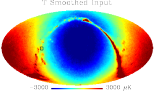
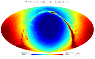
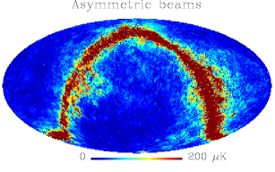
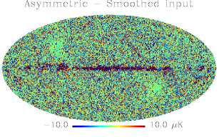
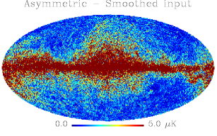
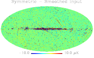
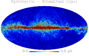
Figure 5: Madam maps made from simulated noiseless TODs. Maps on the left are temperature maps. Those on the right give the magnitude of the polarization vector ($P=\sqrt{Q^{2}+U^{2}}$). All maps contain CMB, dipole and foreground emissions. Top row: Smoothed input maps. Second row: Madam maps. These maps include the effects of asymmetric beams and sample integration. Third row: Difference of the above Madam map and the smoothed input map. Bottom row: Same as above, but for symmetric beams. The maps of the top and second rows are in ecliptic coordinates, whereas the difference maps are in galactic coordinates. The latter coordinates were chosen to give a clearer view to the ecliptic pole regions (see the light green areas of the asymmetric difference map). Small patches of noiseless Madam temperature maps are shown in Figs. 6 and 7.

To demonstrate the effects of beams in our maps, we made maps from the noiseless TODs containing CMB, dipole, and foreground emissions. We show the Madam maps as an example in Fig. 5. Corresponding maps of the other mapmaking codes would look similar. We can hardly see any differences between the noiseless output map and the smoothed input map (see the two upper rows of Fig. 5). To reveal the differences, we subtract the smoothed input map from the output map (bottom two rows of Fig. 5). The beam window functions of the symmetric and asymmetric beams differ mainly at high-$\ell$ (see Sect. 5.1.2), which makes mainly small angular (pixel) scale differences in the maps. Therefore the difference map of the asymmetric beams contains more small-scale residuals than the difference map of the symmetric beams. The ecliptic pole regions of the sky are scanned in several directions, which makes the effective beam of the asymmetric case more symmetric and therefore closer to the effective beam of the symmetric case. Therefore the difference of the noiseless output map of the asymmetric beams and the smoothed input map becomes small in the vicinity of the ecliptic poles (see the light green areas of the difference map of the third row of Fig. 5). The angular diameter of these areas is $\backsim$$30^{\circ}$.

Some point source residues are visible in the temperature difference maps of Fig. 5 (see especially the lower left corner map). A likely reason for these residues is the difference in how the pixel areas are sampled in the output maps and in the smoothed input map. In the latter map the pixel temperature is an integral of the sky temperature over the pixel area, whereas in the output map the pixel temperature is an average of the observations falling in the pixel. The observations do not necessarily sample the pixel area uniformly, which leads to a different pixel temperature than in the uniform integration.

The difference maps of Fig. 5 have some stripes that align with the scan paths between the ecliptic poles. These stripes are most noticeable close to the galactic regions in the symmetric case difference map. In the asymmetric case the stripes do not stand out from the larger pixel scale residuals. They arise from the fact that signal differences (gradients) inside a map pixel create non-zero baselines in Madam that show up as stripes in the Madam map. Because the signal gradients are largest in the galactic regions, the stripes are strongest there. All our mapmaking codes produce such signal errors, which are stronger in the optimal codes than in the destripers (Poutanen et al. Pou06 (2006), Ashdown et al. 2007b ).

Another way to see the effects of the beams in the maps is to examine how point sources show up in the maps. The image of a point source in the map shows the effective beam at that location of the sky. Figs. 6 and 7 show two such point sources of the noiseless Madam temperature maps. Fig. 6 is a patch from the vicinity of the ecliptic plane. There the scanning is mainly in one direction and therefore the difference in ellipticities of the effective beams (of the symmetric and asymmetric cases) is clearly visible. Fig. 7 shows a similar comparison near the south ecliptic pole. Here the wide range of the scanning directions makes the effective beams more symmetric. The effective beams of the symmetric and asymmetric cases are now more alike, but we can still detect some difference in their ellipticities.

In our simulations beams and sample integration distort the TOD before the instrument noise is added. Independent of the noise, these effects are best explored in the binned noiseless maps, independent of any particular mapmaking algorithm. We examine the effects of the beams and sample integration on the binned noiseless maps in Sect. 5.1.

Because the beams and sample integration affect the signal gradients of the observations, they have an impact on the signal error too. We examine these effects in Sect. 5.2, and compare differences between mapmaking codes. It is only through the signal error that the effects of beams and sample integration show up differently in the maps. The binned noiseless map contribution that is also affected by beams and sampling stays the same in all maps. In our simulations beams should have no effect in the residual noise maps. Because there is a half a sample timing offset between the detector pointings of sampling on and off cases, the hit count maps of these two cases differ slightly, which shows up as small differences in the residual noise maps.

Finally we discuss sorption cooler fluctuations and detector pointing errors and assess their impacts in the maps.

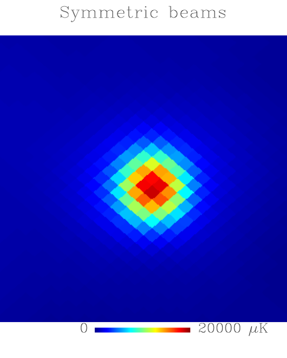
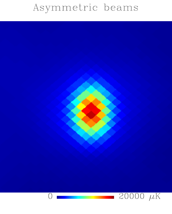
Figure 6: Effect of beams in the point source observations. These plots show $3^{\circ}\times 3^{\circ}$ patches of the noiseless Madam temperature maps (from Fig. 5), zoomed to the vicinity of the ecliptic plane. The location of the patch is given as a square box in the top left map of Fig. 5.

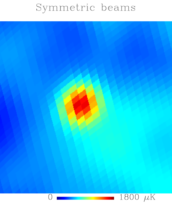
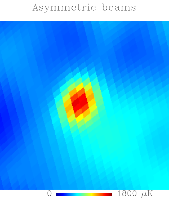
Figure 7: Similar plots as in Fig. 6, but now we have zoomed to a point source near the south ecliptic pole (in $(\lambda,\beta)=(255^{\circ},-81^{\circ})$ of ecliptic longitude and latitude). The size of the patch is $3^{\circ}\times 3^{\circ}$.

5.1 Binned noiseless maps

The effects of beams and sample integration were examined from the binned ($I,Q,U$) maps made from the four noiseless TODs of different beam and sampling cases. The TODs contained only CMB. The angular power spectra of the four maps are shown in Fig. 8. The TT angular power spectra of the symmetric and asymmetric beams differ mainly at large multipoles ($\ell\gtrsim 600$). This is a result of the different effective beam window functions of these two cases.

The EE spectra of symmetric and asymmetric beams are different at both intermediate ($\ell\gtrsim 100$) and high multipoles. Due to the beam mismatch the EE spectrum of the asymmetric beam case is influenced by the cross-coupling from the temperature. A similar cross-coupling does not occur in the symmetric beam case (no beam mismatch). Therefore the EE spectra behave differently than the TT spectra. We discuss these issues more in Sects. 5.1.1 and  5.1.2 and give there the explanation of the behaviors of the TT and EE spectra.

Sample integration is effectively a low-pass filter in the TOD domain. Therefore it introduces an extra spectral smoothing that removes some small-scale signal power from the map. This effect is just barely visible in Fig. 8, where the TT and EE spectra with “sampling” are slightly suppressed as compared to their “no sampling” counterparts. We discuss these effects more in Sect. 5.1.4.

The TT and EE spectra of the binned maps become flat at high $\ell$ ($\gtrsim 1000$). This is a result of spectral aliasing ($\ell$ mode coupling) that arises from the non-uniform sampling of the pixel areas. The aliasing couples power from low-$\ell$ to high-$\ell$. We see this effect in the maps too, where we called it the pixelization error.

Because the CMB input sky contained no $B$-mode power, the signals in the BB spectra of the binned maps (see Fig. 8) must arise from temperature and $E$-mode polarization signals leaking to the $B$-mode. The magnitudes of the symmetric beam BB spectra are comparable to the magnitude of the high-$\ell$ flat part of the corresponding EE spectra. This observation and the fact that the symmetric beams were all identical (no beam mismatch) suggest that the BB spectrum of the symmetric beam case mainly arises from the spectral aliasing from the E mode (due to pixelization error). The BB spectrum of the asymmetric beam case shows a distinct signal at multipoles between 100 and 800. We expect this signal to originate from temperature and $E$-mode polarization signals that cross-couple to BB due to beam mismatch. We discuss these cross-couplings more in Sect. 5.1.1.

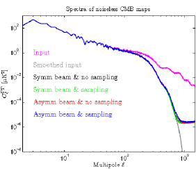
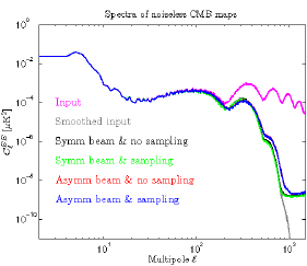
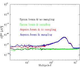
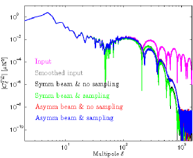
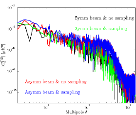
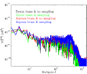
Figure 8: Overview of the effects of beams and sample integration on the angular power spectra of the CMB maps. We computed the spectra of the noiseless CMB maps that were binned from the four simulated LFI 30 GHz TODs. The TODs represent different beam and sample integration cases. The CMB input sky contains no $B$ mode power. Note that the plots of the cross-spectra show their absolute values. In this paper we define $C_{\ell}^{XY}\equiv\frac{1}{2\ell+1}\sum_{m=-\ell}^{\ell}{a_{\ell m}^{X}(a_{\ell m}^{Y})^{\star}}$. Here $X,Y=T,E,B$ and $Z^{\star}$ is the complex conjugate of $Z$.

5.1.1 Beam mismatch, cross-couplings of $I$, $Q$, and $U$

We can quantify the effects of beam mismatch on the maps by calculating power spectra. We consider the asymmetric beam case with no sampling. A number of authors have worked on beam mismatch systematics and their impacts on maps and angular power spectra (Hu et al. Hu03 (2003), Rosset et al. Ros07 (2007), O’Dea et al. Ode07 (2007), Shimon et al. Shi08 (2008)).

The LFI main beams vary in width and orientation from detector to detector. These variations are fully represented in our asymmetric beams. (In contrast, the widths of our symmetric beams were the same in all detectors.) Due to beam mismatch, the detectors of a horn see different Stokes I; this difference appears as an artifact in the polarization map. This is a potentially serious issue for a CMB experiment such as Planck, because the fraction of the strong temperature signal that pollutes the polarization map (denoted $T\rightarrow P$) may be fairly large compared to the weak CMB polarization signal itself.

Strong foreground emission dominates the $T\rightarrow P$ signal in a full sky 30 GHz map. This map is useful for CMB power spectrum estimation only if the pixels with strong foreground contribution are removed from the map (galactic cut); however, the $T\rightarrow P$ signal will depend on the mask used in the cut. To avoid this, and to study the beam mismatch effects in a more general case for which our results would not depend much on the details of the data processing (e.g., masks), we decided to continue to work with the full sky noiseless maps that we binned from the CMB TOD.

To give low-$\ell$ details we replotted the EE and TE spectra (from Fig. 8) of the binned noiseless CMB map (asymmetric beams & no sampling) and the smoothed input map. The replotted spectra are shown in Fig. 9. The $T\rightarrow P$ cross-coupling is a significant systematic for the power spectrum measurement, as Fig. 9 shows. The acoustic peaks and valleys of the binned map are shifted towards higher multipoles. In the EE spectrum the effect is smaller than the noise, and may not be detectable. For the TE spectrum the error of the E mode polarization gets amplified by the large temperature signal. This results in a larger artifact that is visible even in the noisy TE spectrum (see Fig. 20 and the discussion in Sect. 5.2).

We designed a simple analytic model that gives a reasonably good description of the effects of the beam mismatch in the angular power spectra of the ($I,Q,U$) signal maps (Appendix A). Our model shows that the mismatch of the beams of a horn is relevant for $T\rightarrow P$. The beams can be different from horn to horn, but only a weak $T\rightarrow P$ may arise if the two beams of a horn are identical.

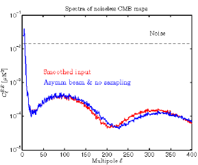
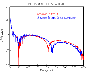
Figure 9: Effects of $T\rightarrow P$ cross-coupling arising from beam mismatches. Left panel: Replot of the EE spectra from Fig. 8, showing spectra of a binned noiseless CMB map (blue curve) and smoothed input map (red curve). The expected EE spectrum of the white noise map is indicated by the horizontal dashed line. Right panel: TE spectra of the same maps. We show the absolute values of the spectra. The TE spectrum does not have a noise bias, because white noise is uncorrelated in the temperature and polarization maps. Therefore the dashed line of noise bias is missing from this plot.

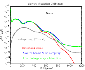
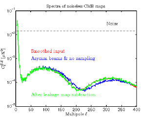
Figure 10: Demonstration of how removing the $T\rightarrow P$ cross-coupling restores the acoustic peaks and valleys of the CMB in their original positions. Left hand panel: We show here a number of EE spectra. The gray curve shows the EE spectrum of the leakage map. The red and blue curves are as in Fig. 9. The green curve shows the spectrum of the binned noiseless map, where the leakage map has first been subtracted. Note that the green curve is nearly on top of the red curve at low multipoles ($\ell<400$). The red and green curves differ at $\ell>450$ mainly due to differences in the beams: the red spectrum is smoothed with symmetric beams while the green spectrum is smoothed with asymmetric beams. At $\ell>1050$ the green and blue spectra become flat due to spectral aliasing arising from pixelisation errors. $T\rightarrow P$ becomes flat too for the same reason. The expected spectrum of the white noise map is indicated by the horizontal dashed line. Right hand panel: Same as left hand panel but zoomed to lower $\ell$. The red and green curves are nearly on top of each other.

To isolate the effect of $T\rightarrow P$, we generated test TODs for all four 30 GHz radiometers. The TODs contained Stokes $I$ of the CMB only. We binned a new $(I,Q,U)$ map from these TODs. The polarization part of the map should contain the temperature leakage only. We therefore call this map the leakage map. The power spectra of the leakage map and the original binned map with the leakage map subtracted are shown in Figs. 10 and 11. Removing $T\rightarrow P$ restores the acoustic peaks and valleys of the EE spectrum in their original positions. The mismatch of the beams is important at or below the beam scale. Therefore the magnitude of the $T\rightarrow P$ leakage, and the corresponding error in the EE spectrum, are small at low $\ell$.

Beam mismatches cause cross-coupling in the opposite direction too, namely $E\rightarrow T$ and $B\rightarrow T$; however, because the E and B mode powers are small compared to the power of the temperature signal, these couplings have an insignificant effect in the maps and angular power spectra.

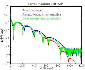
Figure 11: Restoration of the acoustic peaks and valleys in the TE spectrum. Left hand panel: Similar to the left hand panel of Fig. 10, but for TE spectra. Note that we plot the absolute value of the spectra. Right hand side: Same as the left hand panel, but we plot now $\ell(\ell+1)C_{\ell}^{TE}/2\pi$ and zoom to lower multipoles. The red and green curves are nearly on top of each other.

The $B$-mode spectra (left-hand panel of Fig. 12) show two notable effects. First, the cross-coupling from the temperature to the $E$- and $B$-mode spectra are not the same. Though similar in shape, the $T\rightarrow E$ power is 2–3 orders of magnitude larger than the $T\rightarrow B$ power (at $\ell\backsim$ 200). This discrepancy is rooted in the beam widths and orientations coupled with the scan pattern. Our analytic model (of Appendix A) is able to predict this behavior (see the right-hand panel of Fig. 12). The analytic model also shows that if the detector beams were axially symmetric but different in widths, $E$ and $B$ would show the same amount of leakage from temperature.

Second, the $B$-mode spectrum shows more power than can be explained by $T\rightarrow P$ alone (see the green curve of Fig. 12). Because the CMB sky did not contain $B$-mode polarization, the $B$-mode power remaining after the removal of the $T\rightarrow P$ must result from the $E\rightarrow B$ cross-coupling. The source of the distinct $E\rightarrow B$ signal at $\ell<800$ is the spin-flip coupling. In Appendix A we show that the relevant quantity in $E\rightarrow B$ is the sum of the beam responses of the pair of detectors sharing a horn. If there is a mismatch of these sums (mismatch between the horns), the two polarization fields of opposite spins ($Q+iU$ and $Q-iU$) get mixed. This is the spin-flip coupling (Hu et al. Hu03 (2003)). Appendix A shows how the spin-flip coupling arises from the beam mismatch and how it creates $E\rightarrow B$. In these simulations the source of the mismatch of the sum responses is not the widths of the beams, but their orientations (see Sect. 3.2). The widths of the pair of beams of a horn are different, but the pairs of beams have these same values in both horns. The orientations of these pairs are, however, different in the two horns.

In spite of the fact that the CMB $E$-mode polarization signal is significantly weaker than the temperature signal, the magnitude of the $E\rightarrow B$ signal is larger than the magnitude of $T\rightarrow B$ signal. It seems that the difference of the orientations of the pairs of beams produces an $E\rightarrow B$ signal that is stronger than the $T\rightarrow B$ signal produced by the mismatch of widths of the two beams of a horn. The power transfer between the polarization modes operates equally in both directions. $B\rightarrow E$ cross-coupling occurs too (same coupling transfer function as in $E\rightarrow B$), but it has no effect in $E$, because the $B$-mode power is zero. At large multipoles (flat part of the BB spectrum at $\ell>800$) the main source of $E\rightarrow B$ is the $\ell$ mode coupling of the non-uniform sampling of the pixels (pixelization error).

Finally, the $T\rightarrow B$ and $E\rightarrow B$ signals could be compared to the magnitude of the CMB $B$-mode signal that we might expect to detect with LFI 30 GHz detectors. In the right-hand panel of Fig. 12 the leakage spectra are compared to a theoretical BB spectrum of the CMB (including lensing from $E$ mode and corresponding to a 10% tensor-to-scalar ratio). It can be seen that the cross-coupling to $B$ is small compared to this signal for $\ell\leq 300$.

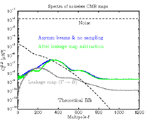
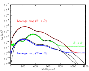
Figure 12: Left hand panel: Effects of $T\rightarrow P$ and $E\rightarrow B$ cross-couplings on the BB spectra. The blue curve is the spectrum of the binned noiseless CMB map. The gray curve is the BB spectrum of the $T\rightarrow P$ leakage map. Because the input CMB sky had zero $B$-mode power, the remaining BB power after the subtraction of the leakage map is mostly cross-coupling from the $E$-mode polarization. This is shown by the green $E\rightarrow B$ curve. The expected spectrum of a white noise map is indicated by the horizontal dashed line. For comparison, we show a theoretical $B$-mode spectrum corresponding to a 10% tensor-to-scalar ratio and including lensing from $E$. Right hand panel: EE and BB spectra of the $T\rightarrow P$ leakage map (red and blue curves, respectively) and the BB spectrum of the $E\rightarrow B$ coupling (green curve). They are the same as the gray and green curves of the left-hand panel of this figure and the gray curve of the left-hand panel of Fig. 10. The thin black lines are the predictions of these signals computed from the analytical model (Appendix A). Flattening at high $\ell$ results from non-uniform pixel sampling. This effect is not included in our model, however, so the model spectra do not become flat.

5.1.2 Effective window functions

The effects of instrument response and data processing on the map can be described in terms of an effective window function, which we compute as the ratio of the map power spectrum to the input spectrum. In our simulations, beams, sample integration, and sampling of the pixel area (pixel window function) are the main contributors to the effective window function. In some cases, to reveal more details, we compute the effective window functions relative to the smoothed input spectrum.

Figure 13 shows the TT, EE, and TE effective window functions of the binned noiseless CMB maps that we introduced earlier in this section. The Gaussian window function approximation breaks down at high $\ell$ and the function becomes flat or starts to increase (as in the TT window functions). This is an effect of the pixelization error in the binned noiseless maps. Polarity changes of the TE spectra cause the sudden jumps seen in the TE window functions. The EE and TE window functions of the asymmetric beams show another non-regular characteristic. They deviate significantly from the regular Gaussian response. The source of this effect is the $T\rightarrow P$ cross-coupling. The magnitudes of the window functions with “sampling on” are systematically smaller than their “sampling off” counterparts. This is more clearly visible in the window functions of the symmetric beams. This difference in window functions comes from the extra spectral smoothing of the sample integration.

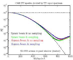
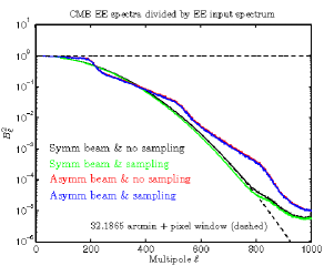
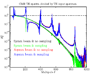
Figure 13: TT, EE, and TE effective window functions, computed as ratios of the angular power spectra of the binned noiseless CMB maps and the input CMB. Because the $B$-mode power of the CMB was zero, no BB window function could be computed. For comparison we show the total response of the axially symmetric Gaussian beam (dashed curve; FWHM = $32\aas@@fstack{\prime}1865$ and $N_{\rm side}$ = 512 HEALPix pixel window function). This is the window function that we applied to the input spectrum to obtain the smoothed input spectrum.

To examine the window functions without the effects of the $T\rightarrow P$ cross-coupling seen above, we subtracted the $T\rightarrow P$ leakage map from the polarization part of the binned noiseless CMB map and recomputed the window functions, as shown in Fig. 14. We did this for the asymmetric beams/no sampling case, because we had the leakage map for this case only. The window functions have now more regular shapes. The TT and EE window functions are not identical; the TT function is slightly steeper than the EE function. In the case of perfectly matched beams the TT and EE window functions would be identical.

The subtraction of the $T\rightarrow P$ leakage map from the binned map does not influence the $E\rightarrow B$ cross-coupling. In addition to creating a $B$-mode polarization signal from the $E$-mode signal, this coupling influences the original $E$-mode signal (see Sect. A.1 of Appendix A), so that the TT and EE window functions become different. Fig. 14 demonstrates that our analytical model is able to explain these window functions.

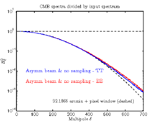
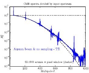
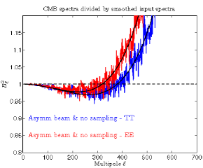
Figure 14: TT, EE, and TE effective window functions after the $T\rightarrow P$ leakage map has been removed from the binned noiseless CMB map (asymmetric beam & no sampling). Top row: The TT window function is the ratio of the power spectra of the binned noiseless CMB map and the CMB input map. The EE and TE window functions were calculated similarly, except that $Q$ and $U$ leakage maps were first subtracted from the original binned noiseless map. Symmetric Gaussian responses were separately fitted to the TT and EE window functions (in range $\ell=0\ldots 500$). The fit FWHM were 32.^′32 (TT) and 31.^′94 (EE). Bottom panel: The TT and EE window functions of the top left panel were divided by the dashed theoretical window function. The resulting ratios are shown in this plot. Thin black curves are window functions that we computed from our analytical model for this case (see Appendix A).

The effective window function of the symmetric beams with no sampling is simple to compute because all detectors have the same beamwidths. If we assume that the scanning is simply from pole to pole and all detector beams have fixed orientations relative to the local meridian, the effective TT window function of the asymmetric beams (no sampling) can be estimated in the following way:

1. Denote by $B_{k}(\theta,\varphi)$ the beam response of the radiometer $k$ of the LFI focalplane (see Fig. 2). The beams are normalized to $\int_{4\pi}{B_{k}(\theta,\varphi)d\Omega}=1$.

2. Compute the coefficients ($b_{\ell m}^{k}$) of the spherical harmonic expansion of the beam $B_{k}(\theta,\varphi)$.

3. Compute the mean $b_{\ell m}$ over the radiometer beams:
   $b_{\ell m}=\frac{1}{N_{\rm det}}\cdot\sum_{k=1}^{N_{\rm det}}{b_{\ell m}^{k}}$. For LFI 30 GHz $N_{\rm det}$ = 4.

4. Compute the effective beam window function as
   $B_{l}^{2}=\frac{4\pi}{2\ell+1}\cdot\sum_{m}|b_{lm}|^{2}$.

If this window function is convolved with the HEALPix pixel window function, the result explains well the TT window function of Fig. 14.

5.1.3 Correction of beam mismatch effects

For temperature observations, the $a_{lm}^{T}$ of the sky get convolved with a beam, which is fully described by one complex number for every $\ell$ and $m$. For polarization, where we need three complex quantities to describe the sky signal ($a_{lm}^{T,E,B}$), the beam in general is a complex $3\times 3$ matrix (for every $\ell$ and $m$). Its non-diagonal elements, which arise from the beam mismatch, are responsible for the cross-couplings of temperature and polarization. The leakage map approach that we used earlier to remove the $T\rightarrow P$ effects is not applicable in real experiments where Stokes $I$-only timelines cannot be constructed independently. For real experiments, more practical methods to correct beam effects are required.

Mapmaking methods that address beam convolution properly have been proposed. Deconvolution mapmaking with a proper treatment of the detector beams is a method to produce maps free from cross-couplings of $T$, $E$, and $B$. Two implementions of this method have been introduced (Armitage and Wandelt Arm04 (2004); Harrison et al. Har08 (2008)). Both have shown results indicating that they may be computationally practical for the lower-resolution Planck channels (in the LFI). Another map-domain method able to correct for beam effects is the FICSBell approach (Hivon et. al. Hiv08 (2008)), in which asymmetries of the main beam are treated as small perturbations from an axially symmetric Gaussian beam, and are averaged over each pixel taking into account the orientation of the detector beams at each visit of that pixel.

In Appendix A we developed an analytical model to predict the effects of the beams in the angular power spectra of the CMB maps. This model was inverted (also in Appendix A) to turn it to a correction method. It can deconvolve the effects of the asymmetric beams from the angular power spectrum and return a spectrum that is an approximation of the spectrum of the input sky. Our method is based on a number of simplifying assumptions that limit its accuracy in real experiments; however, we can use it to compute coarse corrections that can be improved with, e.g., Monte Carlo simulations. The correction capability of our method is demonstrated in Fig. 20.

5.1.4 Sample integration effects

We recomputed the effective TT window functions of Fig. 13, but this time we divided the angular power spectra of the binned noiseless CMB maps with the smoothed input spectrum (instead of the input spectrum). The recomputed effective TT window functions are shown in Fig. 15. A pairwise comparison of the “sampling” and “no sampling” window functions (of the same beam type) reveals the effect of the sample integration in the angular power spectrum of a CMB map. The extra spectral smoothing due to the sample integration can be clearly seen.

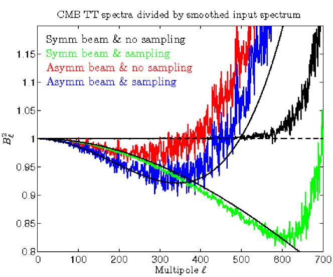
Figure 15: Sample integration effects in the effective TT window functions. These window functions are the ratios of the TT angular spectra of the binned noiseless CMB maps and the smoothed CMB input spectrum. The red curve is the same as the red curve of Fig. 14. The window functions of the symmetric beams (black and green curves) blow up at $\ell\approx 600$ due to pixelization error. The corresponding blow up of the other window functions occurs outside the scales of this plot. The thin black curve that tracks the green curve was computed from Eq. (7). The other black curve (that tracks the blue curve) is the window function prediction of our analytical model multiplied with Eq. (7).

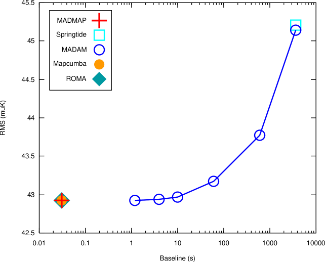
Figure 16: RMS of the residual temperature maps for LFI 30 GHz observations. The maps were $N_{\rm side}=512$ full sky maps and they contained CMB, instrument noise, and the effects of the sorption cooler temperature fluctuations. Asymmetric beams were used, and sample integration was turned on. The y-axis units are thermodynamic microkelvins. The angular power spectra of some of the residual maps are shown in Fig. 17.

Let us consider an axially symmetric Gaussian beam and its elongation in the direction of the scan. The window function of the initial beam (before elongation) is

$$B_{\ell}^{2}=e^{-\ell(\ell+1)\sigma_{0}^{2}},$$ (4)

where $\sigma_{0}=\rm{FWHM}/\sqrt{8\ln 2}$. This window function operates in the angular power spectrum domain. The beam $\sigma$ stays in its original value ($\sigma=\sigma_{0}$) in the perpendicular direction of the scan. Along the scan the $\sigma$ gets modified to (Burigana et al. Bur01 (2001))

$$\sigma_{\rm eff}^{2}=\sigma_{0}^{2}+\frac{\Delta\theta_{\rm s}^{2}}{12}.$$ (5)

Here $\Delta\theta_{\rm s}=2\pi f_{\rm spin}/f_{\rm sample}$, the angle through which the beam center pointing rotates during a detector sample time. For the nominal satellite spin rate ($f_{\rm spin}$ = 1 rpm) the ellipticity ($\sigma_{\rm eff}/\sigma_{0}$) of the elongated beam is 1.027. The ellipticity produced by the scanning is significantly smaller than the ellipticities of our asymmetric beams ($\backsim$1.35).

The geometric mean of the $\sigma$’s of the elongated beam is

$$\sigma_{\rm e}^{2}=\sigma_{0}\sigma_{\rm eff}=\sigma_{0}\sqrt{\sigma_{0}^{2}+\frac{\Delta\theta_{\rm s}^{2}}{12}}\approx\sigma_{0}^{2}+\frac{\Delta\theta_{\rm s}^{2}}{24}.$$ (6)

The last form is an approximation that could be made because $\frac{\Delta\theta_{\rm s}^{2}}{12}\ll\sigma_{0}^{2}$. Eq. (6) suggests that the effect of the sample integration in the angular power spectra of the maps could be approximated by a symmetric Gaussian window function

$$E_{\ell}^{2}=e^{-\ell(\ell+1)\sigma_{\rm s}^{2}},$$ (7)

where $\sigma_{\rm s}=\Delta\theta_{\rm s}/\sqrt{24}$. In our simulations this $\sigma_{\rm s}$ corresponds to FWHM = $5\aas@@fstack{\prime}32$. We compare the predictions of this model to the actual window functions of our simulation in Fig. 15. The comparison shows that the accuracy of our simple model is good in the symmetric beam case but somewhat worse for the asymmetric beam case.

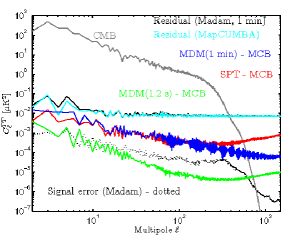
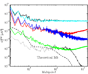
Figure 17: TT, EE, and BB angular power spectra of Madam (with 1-minute baselines and without the noise filter) and MapCUMBA residual maps (black and light blue curves, respectively). Their RMS values were shown in Fig. 16. The maps represent the observations of four LFI 30 GHz detectors (CMB, instrument noise, cooler fluctuations; asymmetric beams; and sample integration on). The red curve is for the difference of the Springtide (SPT) and MapCUMBA (MCB) residual maps. The blue curve is the same for Madam of 1-minute baselines (MDM (1 min)) and MapCUMBA, and the green curve is for Madam of 1.2 s baselines (MDM (1.2 s)) and MapCUMBA. Madam used either 1.2 s or 1-minute baselines, whereas Springtide used long 1 hour baselines. For comparison we also show the CMB spectrum of our simulations (gray curve), the spectrum of the Madam signal error map (including all sky emissions, asymmetric beams, and sample integration, dotted curve), and a theoretical CMB $B$-mode spectrum (dashed curve, see also Fig. 12).

5.2 Residual maps

To compare mapmaking codes, we constructed residual maps, specifically the difference between the output map and the binned noiseless map. Smaller residuals imply smaller mapmaking errors. We examined the RMS of the residuals, and computed power spectra to study scale dependence. We are interested in anisotropy; the mean sky temperature is irrelevant. Therefore, whenever we calculated a map RMS, we subtracted the mean of the observed pixels from the map before squaring. The RMS of a map was always calculated over the observed pixels.

Fig. 16 shows the RMS of the residual temperature maps for some of our mapmaking codes and for a number of destriper (Madam) baseline lengths. The data of Fig. 16 were derived from HEALPix $N_{\rm side}=512$ maps. At that pixel size the instrument noise is the dominant contributor in the residual maps(Poutanen et al. Pou06 (2006), Ashdown et al. 2007b ). The optimal codes consistently deliver output maps with the smallest residuals, which were nearly the same between the several codes. Madam with short uniform baselines (e.g., 1.2 s) produces maps with residuals essentially the same as those of the optimal codes, at considerably lower computational cost. Destriper maps with longer baselines showed larger residuals. The RMS of the other Stokes parameters ($Q$ and $U$) were larger as expected, but behaved similarly as a function of baseline length.

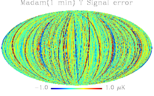
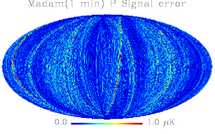
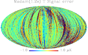
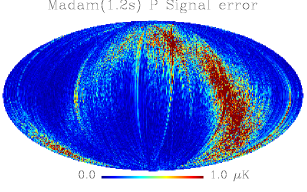
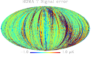
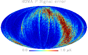
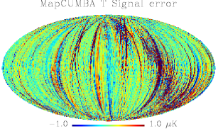
Figure 18: Signal error maps of different mapmaking codes. The signal error is the difference between the noiseless output map and the binned noiseless map. These maps contain all sky emissions (CMB, dipole, and foregrounds) and they are in ecliptic coordinates. The beams were asymmetric and sample integration was off. The left column is for the temperature; the right column is for polarization magnitude. The statistics of these maps are given in Table 3. An example of the effects of beams and sample integration in the signal error maps is shown in Fig. 19.

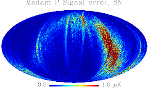
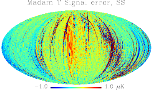
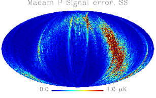
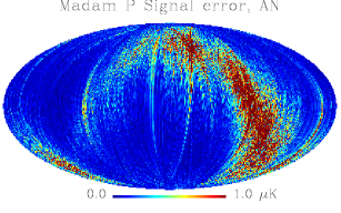
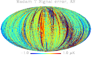
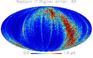
Figure 19: Effects of beams and the sample integration in the signal error maps. We use Madam maps (1.2 s) here as examples. The maps contain all sky emissions and they are in ecliptic coordinates. The left-hand column is for the temperature and the right-hand column is for the polarization magnitude. The rows from the top correspond to symmetric beams & no sampling (SN), symmetric beams & sampling (SS), asymmetric beams & no sampling (AN), and asymmetric beams & sampling (AS). The statistics of these maps are given in Table 4. The third row maps are the same as the second row maps of Fig. 18.

TABLE 3

Statistics of signal error maps^a

      $$I Q U -6.1 3.5 0.415 -1.7 1.5 0.137 -2.4 1.6 0.181 -49.4 20.5 0.890 -7.8 6.5 0.307 -11.3 7.9 0.421 -56.4 21.5 0.910 -8.5 7.0 0.315 -12.5 8.9 0.430 -56.4 21.5 0.910 -8.5 7.0 0.315 -12.5 8.9 0.430$$               Code       MIN       MAX RMS       MIN MAX RMS       MIN MAX RMS Madam (1 min)^b                             Madam (1.2 s)^b                             MapCUMBA                             ROMA                            

^aWe show here the statistics of the signal error maps (given in $$\mu$$K) of different mapmaking codes. This table is for the case of asymmetric beams and sampling off. The corresponding maps are shown in Fig. 18. They contain all sky emissions (CMB, dipole, and foregrounds).

^bWe used Madam in two different configurations: with 1-minute baselines and no noise filter (Madam (1 min)), and with 1.2 s baselines and with noise filter (Madam (1.2 s)).

TABLE 4

Statistics of Madam signal error maps^a

      $$I$$              

TOD       MIN       MAX RMS       MIN MAX RMS       MIN MAX RMS

Symm & no sampling                            

Symm & sampling                            

Asymm & no sampling                            

Asymm & sampling                            

^aThis table shows the effects that beams and sample integration have in the signal error maps. We show here the statistics of Madam (1.2 s) signal error maps (given in $$\mu$$K). The corresponding maps are shown in Fig. 19. They contain all sky emissions (CMB, dipole, and foregrounds). The third line of this table is the same as the second line of Table 3.

The RMS does not provide a complete comparison of map quality. It is weighted toward the high-$\ell$ part of the spectrum, where in any realistic experiment we will be dominated by beam uncertainties and detector noise. Also, since all the errors in the map are folded into a single number, it tends to obscure the origin of the errors. Fig. 17 shows typical angular power spectra of the residual maps. In this plot the Madam (in this case with 1-minute baselines and without noise filter) and MapCUMBA residual spectra are nearly the same. The corresponding spectra of the other mapmaking codes would fall close to them too. To highlight the differences we show the spectra of three difference maps between pairs of residual maps. Green curves show that the difference between Madam (with short baselines) and optimal residual maps is small. Comparison of the blue and red curves shows that destriping with 1-hour baselines (Springtide) produces RMS residuals that are larger than those from the optimal codes, and larger than those from destriping with 1-minute baselines (Madam with 1-minute baselines); the differences are confined to the high-$\ell$ part of the spectrum. At low $\ell$, the codes perform almost identically.

To examine the signal errors of our mapmaking codes we made noiseless maps from the TOD of CMB, dipole, and foreground emissions. We subtracted the corresponding binned noiseless maps from noiseless output maps and obtained the signal error maps. We show some of our signal error maps in Figs. 18 and 19 and their statistics in Tables 3 and 4. In Fig. 18 we show signal error maps of a number of mapmaking methods. These maps were made with asymmetric beams, with sampling off. Their statistics are given in Table 3. Optimal codes and Madam with short baselines (1.2 s) produce nearly the same signal error, which is stronger than the signal error of destripers with long baselines (represented here by another Madam map with 1-minute baselines and no noise filter this time). For optimal and Madam (1.2 s) maps the signal error is more localized to the vicinity of the galaxy (which has strong signal gradients) than for long-baseline destriper maps. Fig. 17 shows that in the high-resolution 30 GHz maps the signal error is a small effect compared to the residual noise or the CMB signal that we used in this study. These results are well in line with the results of our earlier studies (Poutanen et al. Pou06 (2006), Ashdown et al. 2007b ). In the bottom panel of Fig. 17 we compare the Madam signal error with the theoretical CMB $B$-mode spectrum (10 % tensor-to-scalar ratio). The plot shows that the magnitude of the signal error is comparable to the magnitude of this $B$-mode signal. Signal error can therefore limit our possibilities to detect it. In a previous study we examined a number of techniques to decrease the signal error (Ashdown et al. 2007b ). Because the detection of the $B$-mode signal was not a goal of this paper we did not investigate these methods for this data.

Figure 19 and Table 4 show the effects of beams and sample integration on the signal error maps. We use the Madam maps here as examples. The figure and the table show that both switching on the sample integration and switching from symmetric to asymmetric beams increase the signal error. This is because with asymmetric beams also the beam orientation affects the measured signal.

Finally, we turn again to the issue of asymmetric beams, now in the presence of CMB and detector noise. Noise dominates the EE and BB spectra of our observed 30 GHz CMB maps. The TE spectrum, however, does not have a noise bias. Therefore, the effect of the $T\rightarrow P$ cross-coupling can be detected in the noisy TE spectrum. We made a Madam map (with 1-minute baselines and no noise filter) from the TOD of CMB+noise (asymmetric beams and no sample integration). In the TE spectrum of this map, the bias due to $T\rightarrow P$ (arising from the beam mismatch) is clearly visible (see Fig. 20). We can expect that such a large bias will lead to errors in the cosmological studies (e.g., in cosmological parameters), if not corrected. Fig. 20 shows that our analytical correction method developed in Appendix A is able to restore the spectrum, at least on medium and large angular scales (at $\ell\lesssim 450$).

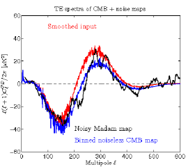
Figure 20: Effects of beam mismatch on the noisy TE spectra. Left hand panel: TE spectrum of a noisy CMB map (Madam map with 1 minute baselines and no noise filter), black curve. To reduce its $\ell$ to $\ell$ variation, it was filtered with a sliding average ($\Delta\ell=20$). TE spectra of the binned noiseless CMB map (blue curve) and the smoothed input map (red curve) are shown too. They are the same curves as in the right-hand panel of Fig. 11. The maps were made with asymmetric beams, and sample integration was off. Right hand panel: Noisy Madam TE spectrum (black curve), where the effects of beam mismatch have been corrected using the analytical method that we developed in Appendix. A.

5.3 Cooler fluctuations

Temperature fluctuations of the Planck sorption cooler were described in Sect. 3.4.2. These fluctuations have an effect in the output signals (TOD) of the LFI 30 GHz radiometers. The typical cooler TOD waveform was shown in Fig. 4. The RMS of this cooler signal is $\backsim$35 $\mu$K, which is about 1/38 of the RMS of the random uncorrelated instrument noise (white noise).

It is of interest to bin the one-year cooler TODs of all four 30 GHz detectors (identical TODs as described in Sect. 3.4.2) in a map, shown in Fig. 21. It looks similar to a map of correlated random noise (with faint stripes along the scan paths). Nutation of the satellite spin axis and the fluctuation of its spin rate (see Sect. 3.1) randomize the regular cooler TOD signal when we project it in the sky. Therefore all map structures that these regularities could produce are washed out. Because a pair of detectors sharing a horn see the same cooler signal, we might expect no cooler effect in the polarization maps. This is not, however, the case in reality. A small polarization signal arises because the polarization axes of the detectors are not exactly orthogonal within a horn (see Table 1).

We made maps of CMB+noise+cooler and CMB+noise. We computed their difference to see the residuals of the cooler fluctuations that our mapmaking codes leave in their output maps. We computed the angular power spectra of these residual maps and show them in Fig. 22. Except for Springtide at small angular scales the residuals of the cooler fluctuations are smaller than signal error. We can therefore conclude, that, in these simulations, the cooler effect is a tiny signal compared to the CMB itself, or to random instrument noise.

The period of the cooler signal is $\backsim$12 min (Fig. 4). Springtide with its long (1 hr) baselines is not able to fit out any cooler power from the observed TOD. Therefore the cooler signal is not suppressed in the Springtide temperature map, but remains in the same level as in the binned cooler map. Springtide uses noise estimates that it computes from its ring maps. Although the TODs of this study have the same noise spectra the white noise levels that Springtide estimates for the rings will be different. The rings are combined using inverse noise variance weighting, and so when rings from two detectors in the same horn (which see the same cooler signal) are not weighted exactly the same, the effect in polarization is enhanced over the binned case which is generated using equal weights. We expect that Springtide would deliver EE and BB cooler spectra that are similar to the binned case if equal weighting would be used.

Madam and the optimal codes, which operate with short baselines (optimal codes have one-sample-long effective baselines), are able to set their baselines to track well the cooler signal and therefore the cooler signal is suppressed in their output maps. Our optimal codes and Madam assumed the same noise spectrum for all TODs. None of them tried to include the cooler spectrum in their noise filters.

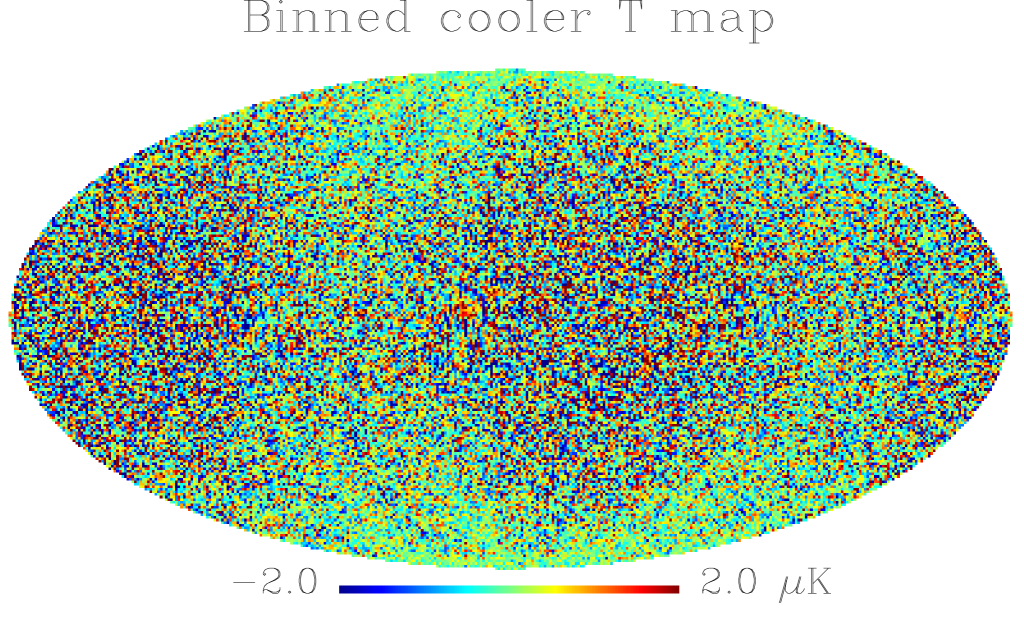
Figure 21: Temperature map binned from the cooler noise TOD. The map is in ecliptic coordinates and it contains observations of all four LFI 30 GHz detectors. Its statistics are (MAX, MIN, RMS) = (10.9, -$11.7$, 1.23) $\mu$K. We do not show the corresponding $Q$ and $U$ maps, but their RMSs were 0.002 and 0.007 $\mu$K, respectively.

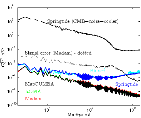
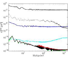
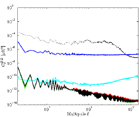
Figure 22: Effect of sorption cooler temperature fluctuations on the CMB maps. These plots show the TT, EE, and BB angular power spectra of residual maps of the cooler effect. The residual maps were computed as differences between the maps of CMB+noise+cooler and CMB+noise. They represent one year of observations of four LFI 30 GHz detectors. The beams were asymmetric and sample integration was on. The light blue curves (“Binned”) show the spectrum of the binned cooler map, whose temperature component is in Fig. 21. Note that the MapCUMBA, ROMA, and Madam curves are nearly on top of each other. For comparison we also show the spectrum of the Springtide CMB+noise+cooler map and the spectrum of the Madam signal error map (including all sky emissions, asymmetric beams, and sample integration, dotted curve, same curve as in Fig. 17).

5.4 Pointing Errors

We modified the Madam destriper in order to quantify how inaccuracy in the knowledge of satellite pointing affects the maps. To isolate this from other effects, we considered first the symmetric-beam, no-sampling case. However, to see the effect on polarization leakage, we needed a reference TOD which contained Stokes I only. This was available only for the asymmetric-beam no-sampling case (see Sec. 5.1.1).

We did not have available a good model for the expected pointing error, but to quantify the magnitude of the effect we considered two opposite schemes: uncorrelated pointing error with a random offset added to the pointing of each detector sample and strongly correlated error for which the offset was kept constant for an hour at a time. The first model is of course unrealistic, but serves to indicate to which direction the effects may change when the offset varies over shorter time scales.

The pointing errors were drawn from a Gaussian distribution so that the RMS error for both the $\theta$ and $\phi$ directions was $\sigma=0\aas@@fstack{\prime}5$. This translates into RMS offset of $\sqrt{2}\sigma$.

The errors were generated independently for each horn; but the two detectors (for the two polarization directions) in the same horn share the same pointing and thus the same pointing error. Thus to a first approximation we would not expect the pointing error to contribute to the temperature-to-polarization leakage. However, since the two polarization directions were not aligned at exactly $90^{\circ}$ to each other, there will be some effect. The different pointing errors of the two horns should contribute to $E\rightarrow B$ leakage.

The $\sigma=0\aas@@fstack{\prime}5$ pointing error led to misplacing 11.5% of the samples into wrong pixels ($N_{\mathrm{side}}=512$ pixels, about $7\arcmin$ across).

In the limit of an infinitely dense, homogeneous hit distribution, a simple model for the pointing errors can be devised. The errors increase the effective size of the pixels, leading to extra smoothing of the output map, similar to smoothing with an axially symmetric Gaussian beam with FWHM $\sqrt{8\ln{2}}\sigma$. In the power spectrum level this means an extra suppression factor of $\exp{\left(-\sigma^{2}\ell(\ell+1)\right)}$.

We defined earlier the residual map as the difference between the output map and the binned noiseless map. Since pointing errors affect also the binned noiseless map, it is not enough to consider the residual map. Therefore we consider here the total error defined as the difference between the output map and the smoothed input map.

Actual measurements typically include inhomogeneous distributions of hits per pixel and within a pixel. Addition of random pointing errors can artificially smooth this distribution, redistributing noise more evenly among the pixels. The expected white noise contribution to the RMS total error is proportional to $\sqrt{\langle 1/N_{\mathrm{obs}}\rangle}$. Random pointing errors may decrease $\langle 1/N_{\mathrm{obs}}\rangle$. Thus random pointing errors may actually reduce the RMS total error in the map. However this does not happen with correlated pointing errors.

Isolated from the redistribution of white noise are the effects on the actual signal. We divide the signal contribution to the total error into two parts: 1) the pixelisation error from uneven sampling of the pixel, defined as the difference (binned noiseless map $-$ smoothed input map); and 2) signal error from destriping, defined as the difference (destriped noiseless map $-$ binned noiseless map). Pointing error affects both differences. The effects of the pointing errors on these different error components are shown in Table 5 for temperature maps. Interestingly, uncorrelated pointing errors also reduced the pixelization error; although the pixel was now sampled from a larger area, apparently the sampling was now more uniform.

The total effect of the $\sigma=0\aas@@fstack{\prime}5$ pointing error was relatively small. In the uncorrelated case, the RMS total error in the map decreased from 43.25 $\mu$K to 43.21 $\mu$K. In the correlated case it increased to 43.30 $\mu$K. These effects are smaller than the difference between the optimal codes and the destriper codes with long baselines (i.e., Madam without noise filter, Springtide).

TABLE 5

Effect of satellite pointing errors on total temperature error maps^a

      Error components $$\sigma 43.2560 42.5449 42.6536 0.5601 7.1663 -0.0432 -0.0279 -0.0318 +0.0023 -0.0611 +0.0482 +0.0222 +0.0166 +0.0383 +0.2047$$       Model       Total error White noise estimate       Residual noise^b Signal error^c Pixelization error^d 0’               0’.5       uncorr.               0’.5       corr.              

^aWe show here how the total RMS error (given in $$\mu$$K) in the map changed by adding pointing errors. This table is for the case of symmetric beams. The first row shows the case without pointing errors. The two other rows show how the map errors changed when adding pointing errors according to the two models considered in Sec. 5.4. The total map error is divided into three parts: residual noise, signal error, and pixelization error, and the effect of pointing error to each part is shown.

^bResidual noise is the power in the difference (destriped map $$-$$ destriped noiseless map). It is dominated by binned white noise.

^cSignal error is the destriping error caused by the signal (destriped noiseless map $$-$$ binned noiseless map).

^dPixelization error is caused by insufficient sampling of the pixel temperature. We measure it from (binned noiseless map $$-$$ smoothed input map).

TABLE 6

Effect of satellite pointing errors on total polarization error maps^a

      Error components

$$\sigma$$       Model       Total error White noise estimate       Residual noise^b Signal error Pixelization error

0’              

0’.5       uncorr.              

0’.5       corr.              

^aWe show here how the total RMS error in the polarization maps changed by adding pointing errors. Polarization error amplitude is the square root of the square sum for the two polarization amplitudes: $$|err_{pol}|=\sqrt{err_{Q}^{2}+err_{U}^{2}}$$.

^bSee Table 5 for the descriptions of the columns.

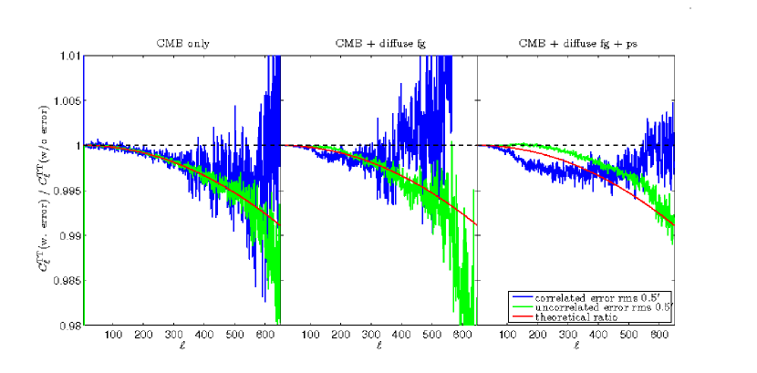
Figure 23: TT power spectra of the $0\aas@@fstack{\prime}5$ pointing error cases divided by the corresponding spectra without pointing errors. All spectra are for the binned noiseless maps (fg = foreground, ps = point source). These plots show that for the CMB only case the pointing errors are well approximated by an effective pixel window (due to larger effective pixel size). However the simple model fails in the presence of secondary signals.

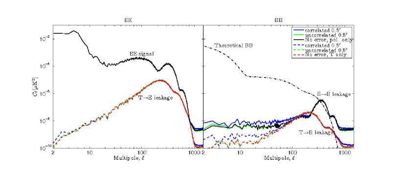
Figure 24: Polarization angular power spectra of the maps made from the noiseless temperature-only TOD and the difference maps between these maps and the ones made from the noiseless TOD with polarization, showing the $E$-mode polarization signal, and the $T\rightarrow E$, $T\rightarrow B$ and the $E\rightarrow B$ leakage effects. For comparison, we show a theoretical B mode spectrum corresponding to a 10% tensor-to-scalar ratio and including lensing from $E$.

We then studied the angular power spectra of noiseless maps binned with additional pointing errors. Should the naive model derived from an infinitely dense homogeneous hit distribution hold, the only difference between spectra from different cases would be the added smoothing. We found this to be the case approximately when binning only the CMB signal. Adding diffuse foregrounds and point sources broke the approximation to a large part, presumably due to sharper structure and lack of statistical isotropy in these foreground components. The decreasing trend from extra smoothing remained still visible. In all cases the random pointing error model corresponded to the smoothing approximation considerably better. The spectra are displayed in Fig. 23. Pointing errors contribute also to the aliasing effect ($\ell$-mode coupling due to uneven distribution of hits), which adds power to high $\ell$, but the effect is negligible in comparison to the residual noise.

For analyzing the effect on polarization maps and power spectra we repeated the study using the asymmetric beam TOD, since for that case a reference TOD containing Stokes I only was available. See Table 6. For correlated pointing errors the increase of the residual noise error is larger by almost an order of magnitude for polarization than for temperature (Table 5). This effect is in line with the estimate based on white noise. The effect is probably due to a relatively small number of pixels where the sampling of polarization directions is not very good, and thus the noise effects get magnified for polarization. The other effects on the map total RMS error are of the same magnitude for polarization maps as for temperature maps.

The $T\rightarrow P$ and $E\rightarrow B$ leakage was studied the same way as in Sect. 5.1.1. The effect of pointing error on this leakage is shown in Fig. 24. The effect on $T\rightarrow E$ leakage is negligible, and the largest effect is on the $E\rightarrow B$ leakage, as anticipated. This should be compared to the magnitude of the kind of $B$ mode we might expect to detect with Planck. In the right-hand panel of Fig. 24 the leakage is compared to the theoretical $B$-mode spectrum that we introduced earlier (see Fig. 12). It can be seen that the leakage to $B$ is small compared to this signal for $\ell\leq 300$. On the other hand, the pointing error effect on this leakage becomes small for $\ell\geq 200$.

Based on these results, pointing errors of $\leq 0\aas@@fstack{\prime}5$ do not appear as a major concern for the 30 GHz channel.

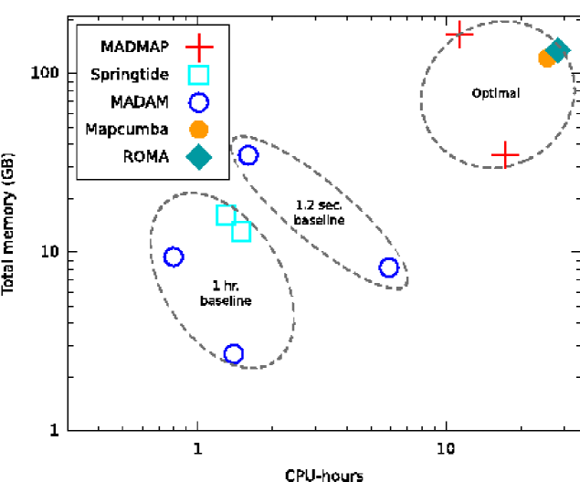
Figure 25: Codes with longer baselines can run with fewer resources. Individual codes can be tuned to be compact in memory or to run quickly.

6 Computing resources

Timing tests of codes were run on the NERSC computer Jacquard, an Opteron cluster running Linux, chosen because it is similar in architecture to the present and future machines in the Planck Data Processing Centers (DPCs). Results are shown in Table 7 and in Fig. 25. Different codes have varying demands for processing power, memory, network interconnect, and disk I/O. Different computers will provide these resources with varying performance, which can make a significant difference in the runtime of a particular code. For this reason, the Jacquard timing tests should be viewed as a useful metric, but not an absolute prediction of performance. Note however that many of the codes perform similar tasks (for example, each must read the TOD), so a change in the performance between machines (in this example, in disk I/O) will have less impact on the relative performance measured between codes. In the real-world application of these codes, they will be tuned to the particular hardware available.

TABLE 7

Resource Requirements^a

      Memory [GB]       Time Code       # Proc.       Per Processor Total       Wall Clock [s] Total [CPU-hr] I/O [CPU-hr] Springtide (A^b).       16       1.0 16.1       293 1.3 …^c Springtide (B).       16       0.8 13.0       336 1.5 … Madam (1-hr baseline, A).       16       0.6 9.4       176 0.8 0.27 Madam (1-hr baseline, B).       16       0.2 2.7       318 1.4 0.64 Madam (1.2 s baseline, A).       16       2.2 34.8       362 1.6 0.23 Madam (1.2 s baseline, B).       16       0.5 8.2       1167 5.9 0.29 MADmap (A).       96       1.7 166.0       427 11.4 0.25 MADmap (B).       32       1.1 35.2       1953 17.4 0.71 MapCUMBA.       64       1.9 122.0       1441 25.6 9.73 ROMA.       64       2.1 134.4       1590 28.3 15.9

^aResults are for runs on the NERSC Jacquard computer. Typical run-to-run variations in total CPU-hours (central processing unit) are 10%, determined from Madam runs. In all tests, $$N_{\rm side}=512 I,Q,U$$ () maps were made from 12 months of simulated observations from four LFI 30 GHz detectors.

^bSeveral codes can trade processing cost for memory usage. For a single code, we mark the timing run optimized for CPU by (A) and the run optimized for memory by (B).

^cIn Springtide, reading the TOD from disk occurs simultaneously with the compression of the TOD to ring-maps. This makes a separate evaluation of the I/O difficult.

TABLE 8

LFI 30 GHz mapmaking Throughput^a

Code Max. Simultaneous Maps       Maps/day^b

Springtide (A) . 8       2359

Springtide (B) . 8       2057

Madam (1-hr baseline, A) . 8       3927

Madam (1-hr baseline, B) . 8       2173

Madam (1.2 s baseline, A) . 4       954

Madam (1.2 s baseline, B) . 8       592

MapCUMBA . 2       119

MADmap (A) . 1       269

MADmap (B) . 4       176

MapCUMBA . 2       119

ROMA . 1       108

^aAssumptions: 1) 128 processors with total 256 GB RAM are allocated to mapmaking ($$\sim$$50% of the LFI DPC goal computer); 2) code performance is taken from Table 7; 3) computer resources are allocated in 16-processor nodes.

^bObtained by dividing the number of seconds in a day by the cpu usage in Table 7, taking into account the number of utilized nodes, processors per node, and number of simultaneous maps.

In early 2009, the LFI DPC will have at least 128 processors with 1 GB per processor (128 GB total memory), with a goal of 256 processors and 2 GB per processor (512 GB total memory), plus 10 TB of disk space. The HFI DPC expects to have 250 processors and 8 GB per processor (2000 GB total memory), plus 200 TB of disk space.

To compare the fast mapmaking capabilities of our codes, we used the data of Table 7 to calculate the rate that 30 GHz maps could be produced in 24 hours, assuming that 50% of the processors and the memory of the LFI DPC goal computer would be available. Results are shown in Table 8. The optimal codes (MADmap, MapCUMBA, ROMA) could produce a couple of hundred maps per day, compared to between several hundred and a couple of thousand for the destripers (Springtide, Madam).

For the LFI and HFI DPCs, the most challenging mapmaking problem is to make a map from 14 months of observations (the nominal Planck mission time) using 12 detectors (the maximum for any channel) at 70 and 217 GHz. We have estimated the total memory and disk space required by the mapmaking codes in these extreme cases.

For the LFI 70 GHz channel, a naive scaling up of the size of the TOD from the 30 GHz timing tests (considering number of detectors, sampling rate, and mission duration) yields total memory requirements 8.3 times those shown in Table 7. The Madam team made more detailed estimates based on counting the size of allocated arrays. For the code running in standard configuration with 1.2-s baselines, the estimate yields a total memory requirement of $\sim 230$ GB, compared to the naive scaling estimate of 270 GB. In split-mode, where the data are first destriped with a 1.2-s baseline in three groups of four detectors, then combined in a second destriping using 1-hr baselines, the memory requirement is 100 GB. For Madam with 1-hr baselines, the memory estimate is 30 GB. In split-mode and for 1-hr baselines, the estimate is less reliable because of uncertainties in the performance of Madam’s data compression system. For a code using the full detector pointing, the disk space required to store the TOD is 0.87 TB. For the compressed satellite pointing sampled at 1 Hz, the requirement drops to 0.12 TB.

For the HFI 217 GHz channel, the naive scaling yields memory requirements 21.5 times those shown in Table 7. The Madam detailed estimate yields 1070 GB for 1.2-s baselines, 460 GB for 1.2-s baselines in split mode, and 100 GB for 1-hr baselines. Using full pointing, the TOD disk requirement is 2.25 TB, but drops to 0.32 TB for compressed pointing.

7 Conclusions

In this paper we have presented results from a simulation that we designed to determine how mapmaking codes handle four aspects of real Planck data: non-axially-symmetric beams, detector sample integration, temperature fluctuations induced by the sorption cooler, and pointing errors. Five mapmaking codes of two basic types (destriping and optimal) were used in this study. We generated one year long streams of observations representing four LFI 30 GHz detectors. This simulation round (Trieste simulation) was number four in a series of mapmaking comparison studies that the Planck CTP group has undertaken.

None of our mapmaking codes made an attempt to deconvolve the beam effects from its output map. Therefore the smoothing effects of the beam and sample integration showed up similarly in all our maps. This is, however, a complicated smoothing, because every map pixel has its own effective beam. We also made a thorough examination of the temperature and polarization cross-couplings that arose from the mismatch of the beams. These effects were also similar in all our maps.

Our conclusions are:

1. Our studies showed that the temperature to polarization cross-coupling of CMB signal caused a detectable bias in the TE spectrum of the CMB map. In the EE spectrum the effect was small compared to the residual noise of the map. The $E\rightarrow B$ cross-coupling of CMB produces a spurious signal whose magnitude in intermediate and large multipoles (at $\ell\geq 300$ in this case) seems to exceed the magnitude of the CMB $B$-mode signal that we might expect to detect with LFI 30 GHz detectors. However, in this range of multipoles the detection of the $B$-mode is difficult due to map noise anyway, and at low multipoles where the signal-to-noise ratio is higher the effect is small. Our study shows that the spectrum biases that $T\rightarrow P$ and $E\rightarrow B$ cross-couplings cause may lead to errors in the cosmological studies, if not corrected. We show a method in this paper that can correct part of these effects in the spectrum domain. Map-domain methods that address the beam convolution issues properly have been proposed by other authors (see Sect. 5.1.3).

2. Signal error (error that mapmaking couples to the output map from the small-scale signal structure) is the part of the output map where beam effects appear differently in the maps of different mapmaking codes. In optimal and short baseline Madam maps this error is larger than in the destriper maps of long baselines (Madam and Springtide). Signal error is, however, a small effect in a high-resolution map if we compare it to the residual noise of the map. Techniques to decrease the signal error were thoroughly examined in our earlier study (Ashdown et al. 2007b ).

3. Based on the results of this study, cooler noise or pointing errors of $\leq 0\aas@@fstack{\prime}5$ do not appear as a major concern for the 30 GHz channel.

Five mapmaking codes (two destripers and three optimal codes) have been developed and compared in four Planck CTP simulation rounds (Cambridge, Helsinki, Paris, and Trieste simulations). We give the following summary of these studies:

1. At the end of a long process, the only essential difference found so far between codes that affects accuracy—as assessed by the RMS residual between an input binned map and the output map—is baseline length, shown in Fig. 16. This assumes that all maps have been made at sufficiently high resolution that the effects of sub-pixel structure are small (see Ashdown et al. 2007b ). (Optimal codes are somewhat more affected [in an RMS residual sense] by sub-pixel structure than are destripers, but this is not an issue at sufficiently high map resolution.) However, the fundamental difference between destriping and optimal codes is in their assumptions about, and handling of, noise. Some of the future tests listed in Sect. 7.1 will probe this difference more intensively than ones performed to date.

2. All optimal codes give essentially indistinguishable results. Madam, a destriper with adjustable baseline length, gives the same result as the optimal codes when the baseline is set short enough. Reliable noise estimation is required for these codes.

3. Resource requirements for the codes vary by more than an order of magnitude in the important categories (memory per processor, total memory, elapsed time, and total CPU-hours), as shown in Table 7 and Fig. 25. Codes set up to deal with pointing information in multiple forms have a practical advantage, in that the resources required in memory, I/O speed, and processor speed can be matched to the resources available (memory, I/O speed, and CPU time).

4. It seems inevitable that Planck will need both a fast and “resource light” mapmaking code for everyday use, and an “ultimate accuracy” but “resource heavy” code, for final data products.

7.1 Future Tests

Our final round of simulations was quite realistic compared to earlier rounds, nevertheless there are still many instrumental and mission effects, both subtle and blatant, that have not been included, some of which are listed below. Further tests of mapmaking must be performed.

• Gaps in TOD.

• High-pass filtering of TOD (e.g., to reduce low frequency noise before mapmaking, to deconvolve the bolometer frequency response in HFI). High-pass filtering will make the noise matrix $\mathbf{C}_{n}$ of Eq. (3) non-diagonal.

• Leakage of galactic temperature signal to the polarization maps due to the bandpass mismatch of the LFI radiometers.

• Beam sidelobes.

• Cross-polarization leakage of the detectors, and polarization angle errors.

• Other forms of random noise (e.g., “popcorn noise”).

• Features in the noise power spectrum (e.g., microphonics, frequency spikes). Note that some of these features may make the noise matrix $\mathbf{C}_{n}$ of Eq. (3) non-diagonal.

• Changes in the baseline signal level (e.g., from telescope emission, background loading of bolometers).

• Realistic pointing errors (errors in the pointing reconstruction)

The scope of this paper was restricted to the mapmaking from the LFI 30 GHz data. The Planck mapmaking codes need, however, to be able to make maps from both LFI and HFI observations. Therefore the list includes mapmaking tests that are relevant for LFI, HFI or both.

Future tests should be run on both a destriping code and an optimal code. As a practical matter, it will be efficient to run the less resource intensive destriping code first to wring out any problems in setting up the test. It is no longer necessary to run tests on multiple implementations of destriping or optimal codes, which have been shown to give the same answer.

Generally speaking, destriping algorithms assume that the noise power spectrum is white at high frequency. The shape of the low frequency power spectrum is not important, so long as the low frequency noise may be fit by a series of offsets (or baselines). The duration of these offsets varies from 1 second to 1 hour in the codes we have tested here, with a trade-off between accuracy and resource usage. For baseline durations longer than 1 minute, destripers need no information about the noise power spectrum. By contrast, the optimal codes are not restricted to white noise at high frequency, but must be informed of the shape of the noise power spectrum.

Deconvolution of a bolometer time constant exercises a difference in these approaches. Bolometers have a response lag to a change in the sky similar to the time for the beam to cross a fixed point. This effect smears the sky image in the direction of the scan. A time stream deconvolution filter, applied prior to mapmaking, can repair this effect on the sky signal, but at the cost of correlating the noise at small scales. We have tested the effect of this with simulated HFI 100 GHz data, where the bolometer time constants are the longest, and where the effect is the most severe (Górski et al. Gor08 (2008)).

Appendix A Effects of beams in the angular power spectrum of a CMB map, an analytic model

In this Appendix we try to explain the mechanisms by which beam mismatches generate cross-couplings between the Stokes $I$, $Q$, and $U$ of a CMB map. We designed a simple analytic model to answer this question. We start by making some simplifying assumptions:

• Scanning is from one ecliptic pole to another along the meridians.

• Sky pixels are observed same number of times by all four LFI 30 GHz detectors.

• All hits fall in the centers of the pixels.

• Detector polarization angles are uniformly spaced in 180^∘ (spacing is 45^∘ for the four 30 GHz detectors).

• Detector noise is white, Gaussian, and every detector has the same noise RMS.

• We consider only the main beams. Far sidelobes are ignored.

• The widths of the main beams are so small that we can apply the small-scale limit and compute the convolution of the beam and sky in the plane wave Fourier space (flat sky approximation).

• Our asymmetric main beams have elliptical Gaussian responses.

The assumptions lead to the following consequences:

• Ellipses are invariant to 180^∘ rotations, therefore the scanning direction does not matter. The results of our model are the same in north-to-south and south-to-north scans.

• In all parts of the sky a detector beam has the same orientation with respect to the local meridian.

• The model does not account for the effects of the pixel sampling (pixel window function and pixelization error).

We expect that in spite of the simplifying assumptions, our model gives a good description of the observations in most parts of the sky. The accuracy of the model should be good in those parts of the sky that are scanned approximately along meridians (ecliptic equator areas). The accuracy of our model may be worse in the ecliptic pole areas, where there is more spread of the scanning directions. In reality, the polar regions with multiple scanning directions are a relatively small fraction of the total sky (see Sect. 5 and the third row of Fig. 5).

The Stokes parameters $Q$ and $U$ at a point in the sky are defined in a reference coordinate system (${\mathbf{e}}_{\theta}$,${\mathbf{e}}_{\phi}$, ${\mathbf{n}}$), where the unit vector ${\mathbf{e}}_{\theta}$ is along the north-south meridian (increasing $\theta$), ${\mathbf{e}}_{\phi}$ is along the increasing $\phi$, and ${\mathbf{n}}$ points to the sky (Górski et al. 2005b ). In this reference coordinate system the polarization angle of a detector is the angle from the local north-south meridian to its polarization sensitive direction (anti-clockwise rotation in the reference coordinate system). The polarization angles of the four detectors (LFI-27a, LFI-27b, LFI-28a, LFI-28b) are $\psi$, $\psi$+90^∘, $\psi$+45^∘, and $\psi$+135^∘. In the north-south scanning the value of $\psi$ is the same as the angle from the scanning direction to the U-axis of LFI-27a (see Fig. 2). This angle is 67 .^∘5 (see the caption of the same figure). For the opposite scanning direction $\psi$ is increased by 180^∘.

The observations from a sky pixel $p$ can be given as

$${\mathbf{y}}({\mathbf{n}}_{p})=\left(\begin{array}[]{c}y_{1}({\mathbf{n}}_{p})\\ y_{2}({\mathbf{n}}_{p})\\ y_{3}({\mathbf{n}}_{p})\\ y_{4}({\mathbf{n}}_{p})\end{array}\right)=\left(\begin{array}[]{c}I_{1}+Q_{1}\cos(2\psi)+U_{1}\sin(2\psi)\\ I_{2}-Q_{2}\cos(2\psi)-U_{2}\sin(2\psi)\\ I_{3}-Q_{3}\cos(2\psi)+U_{3}\sin(2\psi)\\ I_{4}+Q_{4}\cos(2\psi)-U_{4}\sin(2\psi)\end{array}\right)=$$ (16)

$$=\left(\begin{array}[]{c}I_{1}+e^{-i2\psi}\cdot Z_{1}/2+e^{+i2\psi}\cdot Z^{\star}_{1}/2\\ I_{2}-e^{-i2\psi}\cdot Z_{2}/2-e^{+i2\psi}\cdot Z^{\star}_{2}/2\\ I_{3}-ie^{-i2\psi}\cdot Z_{3}/2+ie^{+i2\psi}\cdot Z^{\star}_{3}/2\\ I_{4}+ie^{-i2\psi}\cdot Z_{4}/2-ie^{+i2\psi}\dot{Z}^{\star}_{4}/2\end{array}\right).$$ (21)

Here indices (1,2,3,4) refer to the detectors (LFI-27a, LFI-27b, LFI-28a, LFI-28b), $X^{\star}$ is the complex conjugate of $X$, $Z\equiv Q+iU$ is the complex polarization field, and $Z^{\star}\equiv Q-iU$. In our model the detectors measure different values of the Stokes parameters from the same point of the sky, because their beams are different. The observations stay the same in both scanning directions, because the beams have 180^∘ rotational symmetry and a change of $\psi$ by 180^∘ does not change anything in Eq. (21).

Let us define a “pointing matrix” $\mathbf{A}$

$$\mathbf{A}\equiv\left(\begin{array}[]{ccc}1&e^{-i2\psi}&e^{+i2\psi}\\ 1&-e^{-i2\psi}&-e^{+i2\psi}\\ 1&-ie^{-i2\psi}&ie^{+i2\psi}\\ 1&ie^{-i2\psi}&-ie^{+i2\psi}\\ \end{array}\right)$$ (22)

and a Stokes triplet ${\mathbf{s}}_{p}$ of the pixel $p$

$${\mathbf{s}}_{p}\equiv\left(\begin{array}[]{c}I({\mathbf{n}}_{p})\\ Z({\mathbf{n}}_{p})\\ Z^{\star}({\mathbf{n}}_{p})\\ \end{array}\right).$$ (23)

The unit vector ${\mathbf{n}}_{p}$ points to the center of the pixel.

For uniform white Gaussian noise, the Stokes map ($\hat{{\mathbf{s}}}_{p}$) can be recovered from the detector observations as (Tegmark Teg97 (1997))

$$\hat{{\mathbf{s}}}_{p}=\left(\mathbf{A}^{\dagger}\mathbf{A}\right)^{-1}\mathbf{A}^{\dagger}{\mathbf{y}}({\mathbf{n}}_{p}).$$ (24)

Here $\mathbf{X}^{\dagger}$ is the hermitian conjugate of matrix $\mathbf{X}$. Matrix $\mathbf{A}^{\dagger}\mathbf{A}$ is the $\mathbf{N}_{\rm obs}$ matrix of the pixel $p$ (see the footnote of Sect. 5). The assumptions that we made in the beginning of this Appendix lead to diagonal $\mathbf{N}_{\rm obs}$ ($\mathbf{A}^{\dagger}\mathbf{A}=diag[4,1,1]$).

We can now solve $\hat{I}({\mathbf{n}}_{p})$ and $\hat{Z}({\mathbf{n}}_{p})$ from Eq. (24).

$$\hat{I}({\mathbf{n}}_{p})=\frac{\left(I_{1}+I_{2}+I_{3}+I_{4}\right)}{4}+\frac{e^{-i2\psi}\left[(Z_{1}-Z_{2})-i(Z_{3}-Z_{4})\right]}{8}+$$

$$+\frac{e^{+i2\psi}\left[(Z^{\star}_{1}-Z^{\star}_{2})+i(Z^{\star}_{3}-Z^{\star}_{4})\right]}{8}$$

(25)

$$\hat{Z}({\mathbf{n}}_{p})=\frac{\left(Z_{1}+Z_{2}+Z_{3}+Z_{4}\right)}{4}+\frac{e^{+i2\psi}\left[(I_{1}-I_{2})+i(I_{3}-I_{4})\right]}{2}+$$

$$+\frac{e^{+i4\psi}\left[(Z^{\star}_{1}+Z^{\star}_{2})-(Z^{\star}_{3}+Z^{\star}_{4})\right]}{4}.$$

(26)

The first terms on the right hand sides (of Eqs. (25) and (26)) provide the temperature and polarization signals that we want. The other terms of Eq. (25) represent the cross-coupling of polarization signal to the temperature. This cross-coupling can usually be ignored because the coupling coefficient is typically small and the polarization signal is weaker than the temperature signal.

The second and the third terms of Eq. (26) correspond to $T\rightarrow P$ and spin-flip coupling errors (Hu et al. Hu03 (2003)). The second term shows that the temperature signal can pollute the polarization signal if the beams of the two detectors sharing a horn do not match. Beams can be different from horn to horn, but no leakage of temperature to polarization occurs as long as the beams of a horn are identical.

The spin-flip term (the third term of Eq. (26)) produces cross-coupling between $E$- and $B$-mode polarizations. We show it later in this Appendix. In our model spin-flip coupling occurs if there is a horn-to-horn mismatch between the total beams. Here the total beam means the sum of the responses of the two beams of a horn.

Convolution of the detector beam and the sky produces the observed temperature and polarization fields ($I_{1},Z_{1},I_{2},Z_{2},I_{3},Z_{3},I_{4},Z_{4}$). We assumed that this convolution can be computed as a multiplication between the corresponding flat-sky Fourier-domain quantities. This is a good approximation in a small flat patch around the point of observation. We can therefore write $I_{1}({\mathbf{k}})=B_{1}({\mathbf{k}})I({\mathbf{k}})$, $Z_{1}({\mathbf{k}})=B_{1}({\mathbf{k}})Z({\mathbf{k}})$, $I_{2}({\mathbf{k}})=B_{2}({\mathbf{k}})I({\mathbf{k}})$, $Z_{2}({\mathbf{k}})=B_{2}({\mathbf{k}})Z({\mathbf{k}})$ and so on. Here ${\mathbf{k}}$ is the 2-dimensional plane wave vector and ($B_{1}({\mathbf{k}})$, $B_{2}({\mathbf{k}})$, $B_{3}({\mathbf{k}})$,$B_{4}({\mathbf{k}})$) are the Fourier-domain representations of the (flat-sky) responses of the (LFI-27a, LFI-27b, LFI-28a, LFI-28b) main beams. Because we assumed ideal elliptic Gaussian main beams, their functional forms are well known and they are real-valued for all widths, ellipticities and orientations (Fosalba et al. Fos02 (2002)). The Stokes parameters of the sky are given by $I({\mathbf{k}})$ and $Z({\mathbf{k}})$.

We can now write the relation between the Stokes parameters of the map and those of the sky (for Fourier-domain quantities):

$$\left(\begin{array}[]{c}\hat{I}({\mathbf{k}})\\ \hat{Z}({\mathbf{k}})\\ \hat{Z}^{\star}({\mathbf{k}})\\ \end{array}\right)=\left(\begin{array}[]{ccc}B_{\rm s}/4&e^{-i2\psi}B^{\star}_{\rm c}/8&e^{+i2\psi}B_{\rm c}/8\\ e^{+i2\psi}B_{\rm c}/2&B_{\rm s}/4&e^{+i4\psi}B_{\rm d}/4\\ e^{-i2\psi}B^{\star}_{\rm c}/2&e^{-i4\psi}B_{\rm d}/4&B_{\rm s}/4\\ \end{array}\right)\cdot\left(\begin{array}[]{c}I({\mathbf{k}})\\ Z({\mathbf{k}})\\ Z^{\star}({\mathbf{k}})\\ \end{array}\right).$$ (27)

Here $B_{\rm s}$, $B_{\rm d}$, and $B_{\rm c}$ are Fourier-domain quantities and they are defined in terms of the beam responses

$$B_{\rm s}({\mathbf{k}})\equiv B_{1}({\mathbf{k}})+B_{2}({\mathbf{k}})+B_{3}({\mathbf{k}})+B_{4}({\mathbf{k}})$$ (28)

$$B_{\rm d}({\mathbf{k}})\equiv B_{1}({\mathbf{k}})+B_{2}({\mathbf{k}})-B_{3}({\mathbf{k}})-B_{4}({\mathbf{k}})$$ (29)

$$B_{\rm c}({\mathbf{k}})\equiv\left(B_{1}({\mathbf{k}})-B_{2}({\mathbf{k}})\right)+i\left(B_{3}({\mathbf{k}})-B_{4}({\mathbf{k}})\right).$$ (30)

$$B^{\star}_{\rm c}({\mathbf{k}})\equiv\left(B_{1}({\mathbf{k}})-B_{2}({\mathbf{k}})\right)-i\left(B_{3}({\mathbf{k}})-B_{4}({\mathbf{k}})\right).$$ (31)

The 3$\times$3 matrix of the right-hand side of Eq. (27) gives the mapping from the Stokes parameters of the sky to the Stokes parameters of our map. We can therefore call it the Mueller matrix. We use the symbol $\mathbf{M}({\mathbf{k}})$ for it here. In a real experiment each pixel of the map has its own Mueller matrix, because detector hit counts, sampling of pixel area, and beam orientations are different for different pixels. Our model, however, leads to one Mueller matrix that applies in all pixels of the sky.

Next we make the connection between the polarization field ($Z({\mathbf{k}})$) and the fields of the $E$- and $B$-mode polarization ($E({\mathbf{k}})$ and $B({\mathbf{k}})$) (Zaldarriaga & Seljak Zal97 (1997)). We include the temperature anisotropy field ($I({\mathbf{k}}$)) in these equations.

$$\left(\begin{array}[]{c}I({\mathbf{k}})\\ Z({\mathbf{k}})\\ Z^{\star}({\mathbf{k}})\\ \end{array}\right)=\left(\begin{array}[]{ccc}1&0&0\\ 0&e^{+i2\phi_{{\mathbf{k}}}}&ie^{+i2\phi_{{\mathbf{k}}}}\\ 0&e^{-i2\phi_{{\mathbf{k}}}}&-ie^{-i2\phi_{{\mathbf{k}}}}\\ \end{array}\right)\cdot\left(\begin{array}[]{c}I({\mathbf{k}})\\ E({\mathbf{k}})\\ B({\mathbf{k}})\\ \end{array}\right)=$$ (41)

$$=\mathbf{R}\left(\phi_{{\mathbf{k}}}\right)\cdot\left(\begin{array}[]{c}I({\mathbf{k}})\\ E({\mathbf{k}})\\ B({\mathbf{k}})\\ \end{array}\right).$$ (45)

Here the angle $\phi_{{\mathbf{k}}}$ is defined through ${\mathbf{k}}=\left(k_{x},k_{y}\right)=k\left(\cos(\phi_{{\mathbf{k}}}),\sin(\phi_{{\mathbf{k}}})\right)$ and $k\equiv|{\mathbf{k}}|$ is the magnitude of the wave vector. The definition of the 3$\times$3 matrix $\mathbf{R}\left(\phi_{{\mathbf{k}}}\right)$ is evident from the equation.

We assume that the sky emission (like the CMB) is statistically isotropic. Therefore the ensemble mean of its power spectrum does not depend on the direction of ${\mathbf{k}}$ and it can be computed in a $3\times 3$ matrix form

$$\mathbf{C}(k)\equiv\left(\begin{array}[]{ccc}C^{TT}(k)&C^{TE}(k)&C^{TB}(k)\\ C^{TE}(k)&C^{EE}(k)&C^{EB}(k)\\ C^{TB}(k)&C^{EB}(k)&C^{BB}(k)\\ \end{array}\right)=\left\langle\left(\begin{array}[]{c}I({\mathbf{k}})\\ E({\mathbf{k}})\\ B({\mathbf{k}})\\ \end{array}\right)\left(\begin{array}[]{c}I({\mathbf{k}})\\ E({\mathbf{k}})\\ B({\mathbf{k}})\\ \end{array}\right)^{\dagger}\right\rangle.$$ (46)

Here $\langle X\rangle$ is the ensemble mean of $X$. We can now compute the ensemble mean of the power spectrum matrix of the observed map as

$$\left\langle\hat{\mathbf{C}}(k)\right\rangle=\frac{1}{2\pi}\int_{0}^{2\pi}\left\langle\left(\begin{array}[]{c}\hat{I}({\mathbf{k}})\\ \hat{E}({\mathbf{k}})\\ \hat{B}({\mathbf{k}})\\ \end{array}\right)\left(\begin{array}[]{c}\hat{I}({\mathbf{k}})\\ \hat{E}({\mathbf{k}})\\ \hat{B}({\mathbf{k}})\\ \end{array}\right)^{\dagger}\right\rangle d\phi_{{\mathbf{k}}}.$$ (47)

Eqs. (27) and (45) give a relation between ($I,E,B$) of the sky and ($\hat{I},\hat{E},\hat{B}$) of our map. With the help of this relation, we can write an equation that gives us the power spectrum of our map if we know the power spectrum of the sky.

$$\left\langle\hat{\mathbf{C}}(k)\right\rangle=\frac{1}{2\pi}\int_{0}^{2\pi}\mathbf{R}^{\dagger}(\phi_{{\mathbf{k}}})\cdot\mathbf{M}({\mathbf{k}})\cdot\mathbf{R}(\phi_{{\mathbf{k}}})\cdot\mathbf{C}(k)\cdot$$

$$\cdot\mathbf{R}(\phi_{{\mathbf{k}}})\cdot\mathbf{M}^{\dagger}({\mathbf{k}})\cdot\mathbf{R}^{\dagger}(\phi_{{\mathbf{k}}})\cdot d\phi_{{\mathbf{k}}}.$$ (48)

The $3\times 3$ power spectrum matrix is symmetric. It therefore contains 6 different component spectra $C^{XY}(k)$. We can arrange the power spectra of the input sky in a 6-element column vector

$${\mathbf{c}}(k)\equiv\left(\begin{array}[]{c}C^{TT}(k)\\ C^{TE}(k)\\ C^{TB}(k)\\ C^{EE}(k)\\ C^{EB}(k)\\ C^{BB}(k)\\ \end{array}\right).$$ (49)

Similarly we can build a 6-element column vector ${\mathbf{\hat{c}}}(k)$ of the power spectra of the observed map. Because the power spectrum of the input sky does not depend on the direction of the wave vector, Eq. (48) allows us to construct a $6\times 6$ window matrix that, when applied to the spectrum ${\mathbf{c}}(k)$ of the input sky, gives the spectrum ${\mathbf{\hat{c}}}(k)$ of the observed map.

We can use the above results to predict the angular power spectrum (spherical harmonic domain) of our map, if we know the angular power spectrum of the sky. The predicted spectrum will include the effects of the beams, but it will not include the effects from the sampling of the pixel areas (pixel window function and pixelization error). The steps to compute the angular power spectrum prediction are the following.

1. Assume that we know the angular power spectrum multipoles of the input sky. Arrange them in a 6-element column vector at every multipole $\ell$ (as in Eq. (49)).

2. The magnitude $k$ of the Fourier wave vector is the continuous limit of the integer $\ell$ labeling the spherical harmonics multipoles $a_{\ell m}$.

3. For a given multipole $\ell$, set $k=\ell$ in the Mueller matrix $\mathbf{M}({\mathbf{k}})$.

4. For the same multipole, step the angle $\phi_{{\mathbf{k}}}$ from 0 to 2$\pi$ and compute the $6\times 6$ window matrix from the integral of Eq. (48).

5. Apply the window matrix to the angular power spectrum vector of the input sky. The result is the angular power spectrum vector of the observed map (of the same multipole $\ell$).

6. Repeat the previous steps to all multipoles of interest.

Temperature to polarization cross-coupling is an important effect of the beam mismatch. We can use the above procedure to predict this effect too. Instead of using the full 6-element input spectrum vector, we use a vector all of whose elements except $C^{TT}$ are zero, and carry out the prediction steps as before.

We can invert the $6\times 6$ window matrix and compute a corrected angular power spectrum from the spectrum of the observed map. In the corrected spectrum the beam effects have been deconvolved out and it is an approximation of the spectrum of the input sky.

We made a software code that implements the above prediction and correction steps. Instead of building 6-element power spectrum vectors, we assigned the full $3\times 3$ power spectrum matrix column-wise in the vector ${\mathbf{c}}(k)$. This leads to 9-element power spectrum vectors and $9\times 9$ window matrices. They have unnecessary redundancy, but this approach makes the implementation simple and straightforward. The extra computational cost of larger vectors and matrices is unimportant.

Using Eq. (48) we can compute the $9\times 9$ window matrix (see Appendix A of Hamimeche & Lewis Ham08 (2008) for relevant equations of matrix vectorization)

$$\mathbf{W}(k)=\frac{1}{2\pi}\int_{0}^{2\pi}\left(\begin{array}[]{ccc}S_{11}\cdot\mathbf{S}&S_{12}\cdot\mathbf{S}&S_{13}\cdot\mathbf{S}\\ S_{21}\cdot\mathbf{S}&S_{22}\cdot\mathbf{S}&S_{23}\cdot\mathbf{S}\\ S_{31}\cdot\mathbf{S}&S_{32}\cdot\mathbf{S}&S_{33}\cdot\mathbf{S}\\ \end{array}\right)\cdot d\phi_{{\mathbf{k}}}.$$ (50)

Here $\mathbf{S}=\mathbf{S}({\mathbf{k}})\equiv\mathbf{R}^{\dagger}(\phi_{{\mathbf{k}}})\cdot\mathbf{M}({\mathbf{k}})\cdot\mathbf{R}(\phi_{{\mathbf{k}}})$ is a $3\times 3$ matrix (from Eq. (48)) and $S_{ij}=S_{ij}({\mathbf{k}})$ are its elements. The predicted spectrum of the observed map (from the spectrum of the input sky) becomes now

$${\mathbf{\hat{c}}}(k)=\mathbf{W}(k)\cdot{\mathbf{c}}(k).$$ (51)

We further convolved the predicted spectra with HEALPix pixel window function to model the smoothing due to sampling of the pixel area.

The prediction equation (Eq. (51)) is simple to invert for the correction. Before applying the inverse $\mathbf{W}(k)$ to the spectrum of the observed map, we deconvolved the observed spectrum with the HEALPix pixel window function.

We used this code in Sect. 5 of this paper and computed predictions from the input spectrum and corrections from the map spectrum. These predictions we used to explain the beam mismatch effects and beam window functions that we detected in the spectra of our CMB maps. The correction capability of our model is demonstrated in Fig. 20.

A.1 Spin-flip coupling

If the (2,3) and (3,2) elements of the Mueller matrix are non-zero (see Eq. (27)), $Z^{\star}$ will mix with $Z$ and vice versa. This is the spin-flip coupling (Hu et al. Hu03 (2003)). It generates a $B$-mode in the map even if the input sky has no $B$-mode power in it (like the CMB sky of this study). We can describe this situation with the following general expression (for the Fourier-domain quantities)

$$\left(\begin{array}[]{c}\hat{Z}\\ \hat{Z}^{\star}\\ \end{array}\right)=\left(\begin{array}[]{cc}a&b\\ b^{\star}&a\\ \end{array}\right)\cdot\left(\begin{array}[]{c}Z\\ Z^{\star}\\ \end{array}\right).$$ (52)

We assume that $a$ is real as the (2,2) and (3,3) elements of the Mueller matrix (see Eq. (27)). The quantity $b$ and its complex conjugate represent the (2,3) and (3,2) elements of the Mueller matrix. If we assume that the input sky contains no $B$ mode power (ie. $Z$ and $Z^{\star}$ arise from $E$ mode only), we can write for the $E$ and $B$ modes of the mixed fields $\hat{Z}$ and $\hat{Z}^{\star}$ (use Eq. (45) for the relation between the $E$ and $B$ modes and the complex polarization fields)

$$\left(\begin{array}[]{c}\hat{E}\\ \hat{B}\\ \end{array}\right)=\left(\begin{array}[]{cc}e^{+i2\phi_{{\mathbf{k}}}}&ie^{+i2\phi_{{\mathbf{k}}}}\\ e^{-i2\phi_{{\mathbf{k}}}}&-ie^{-i2\phi_{{\mathbf{k}}}}\\ \end{array}\right)^{-1}\cdot\left(\begin{array}[]{cc}a&b\\ b^{\star}&a\\ \end{array}\right)\cdot$$ (59)

$$\cdot\left(\begin{array}[]{cc}e^{+i2\phi_{{\mathbf{k}}}}&ie^{+i2\phi_{{\mathbf{k}}}}\\ e^{-i2\phi_{{\mathbf{k}}}}&-ie^{-i2\phi_{{\mathbf{k}}}}\\ \end{array}\right)\cdot\left(\begin{array}[]{c}E\\ 0\\ \end{array}\right).$$ (64)

This equation can be put in the following form

$$\left(\begin{array}[]{c}\hat{E}\\ \hat{B}\\ \end{array}\right)=\left(\begin{array}[]{c}a\\ 0\\ \end{array}\right)E+\frac{1}{2}\left(\begin{array}[]{c}b^{\star}e^{+i4\phi_{{\mathbf{k}}}}+be^{-i4\phi_{{\mathbf{k}}}}\\ i\left(b^{\star}e^{+i4\phi_{{\mathbf{k}}}}-be^{-i4\phi_{{\mathbf{k}}}}\right)\\ \end{array}\right)E.$$ (65)

The equation shows that spin-flip coupling (non-zero $b$) creates $B$ mode in the mixed field. In addition, the spin-flip coupling influences the $E$ mode itself in the sense that $\hat{E}$ of $b=0$ and $\hat{E}$ of $b\neq 0$ are different.