Abstract

It has recently been shown that the Einstein equation can be derived by demanding a non-equilibrium entropy balance law $dS=\delta Q/T+d_{i}S$ hold for all local acceleration horizons through each point in spacetime. The entropy change $dS$ is proportional to the change in horizon area while $\delta Q$ and $T$ are the energy flux across the horizon and Unruh temperature seen by an accelerating observer just inside the horizon. The internal entropy production term $d_{i}S$ is proportional to the squared shear of the horizon and the ratio of the proportionality constant to the area entropy density is $\hbar/4\pi$. Here we will show that this derivation can be reformulated in the language of hydrodynamics. We postulate that the vacuum thermal state in the Rindler wedge of spacetime obeys the holographic principle. Hydrodynamic perturbations of this state exist and are manifested in the dynamics of a stretched horizon fluid at the horizon boundary. Using the equations of hydrodynamics we derive the entropy balance law and show the Einstein equation is a consequence of vacuum hydrodynamics. This result implies that $\hbar/4\pi$ is the shear viscosity to entropy density ratio of the local vacuum thermal state. The value $\hbar/4\pi$ has attracted much attention as the shear viscosity to entropy density ratio for all gauge theories with an Einstein gravity dual. It has also been conjectured as the universal lower bound on the ratio. We argue that our picture of the vacuum thermal state is consistent with the physics of the gauge/gravity dualities and then consider possible applications to open questions.

1 Introduction

One important clue about the nature of quantum gravity is that the Einstein field equation and quantum field theory in curved spacetime imply that black holes behave as thermodynamical objects consistent with the four laws of thermodynamics. They are endowed with an entropy proportional to the cross-sectional area of the event horizon [1] and a temperature due to quantum Hawking radiation [2]. Although this interplay of gravitation, quantum field theory, and thermodynamics has been a focus of research for over 30 years, it has yet to be completely understood. One fascinating idea was the proposal by Jacobson [3] to reverse the logic of black hole thermodynamics and derive the Einstein equations as a consequence of spacetime thermodynamics and quantum field theory. The idea is that the local acceleration horizons that exist through every point in spacetime are analogous to tiny pieces of a black hole event horizon and have an entropy proportional to their area. The equivalence principle is then invoked to view the local neighborhood around any point in a general curved spacetime as a piece of flat spacetime. Even in flat spacetime accelerated observers can never receive information from certain regions. For these observers, quantum fields are localized to the Rindler wedge of flat spacetime and they view the usual Minkowski vacuum as precisely a thermal state [4, 5]. This supplies the notion of a local temperature. By demanding the Clausius relation $dS=\delta Q/T$ at every point, where $\delta Q$ is the flow of energy across the horizon and $T$ is the Unruh temperature, Jacobson was able to show the Einstein equation appears as an equation of state. This derivation supports the idea that macroscopic spacetime dynamics is just the thermodynamics of the quantum vacuum. In the past several years other related work has shown that in certain spacetimes (spherically symmetric, axisymmetric, and cosmological) the gravitational field equations near a horizon can also be re-expressed as the thermodynamic identity $TdS=dE+pdV$ [6, 7]. These results have deep implications, but their true significance (if any) is not yet clear.

Recently, in order to probe Jacobson’s derivation further, a horizon entropy proportional to a function of the Ricci scalar was considered [8]. The idea was to determine whether higher curvature correction terms that one expects from effective field theory to appear in the gravitational field equation (or action) can be derived from the thermodynamical prescription. It was found that the field equations of $f(R)$ gravity can be derived only if the setting is shifted from equilibrium to non-equilibrium thermodynamics. An extra internal entropy production term proportional to the squared expansion of the horizon is required for the Clausius relation (or now more properly the entropy balance law) to hold. Perhaps more importantly, it was realized that the original derivation of the Einstein equation via an area entropy can be easily generalized to a non-equilibrium setting. In this case an entropy production term proportional to the squared shear of the horizon appears when the entropy balance law holds. Consistency with the Einstein equation requires that the ratio of the shear term coefficient to area entropy density be $\hbar/4\pi$.

The purpose of this paper is to explore the meaning of these additional terms. The existence of entropy production terms proportional to squared shear and expansion is reminiscent of the shear and bulk viscosity terms that appear in viscous fluid hydrodynamics. A connection between horizon dynamics and fluid dynamics was first noticed by Damour [10]. In the 1980’s Price, Thorne, and collaborators further developed this picture into the black hole “membrane paradigm” [11], using a timelike stretched horizon to approximate the null horizon. The shear and expansion of the horizon also appear in the membrane paradigm, where they are interpreted to be viscous terms in the law describing how the horizon area/entropy changes. However, this interpretation is just an analogy and it is not clear if there is a deep relationship between the dynamics of causal horizons and hydrodynamics. If there is a relationship we must not only understand horizons as a fluid system, but also the physics of this system must be consistent with hydrodynamics as an effective theory. In hydrodynamics, viscosities are phenomenological coefficients in the linear constitutive relations between fluxes of momentum in the fluid and the thermodynamic “forces” given by gradients of the fluid velocity. These velocity gradients must be small (both in space and time) compared to some microscopic scale for hydrodynamics to be an accurate description of the near-equilibrium physics.

After reviewing the thermodynamic derivation in detail we will show that it can be consistently reformulated in the language of hydrodynamics. We argue the Minkowski vacuum, which is a thermal state when localized in the Rindler wedge of spacetime, is holographic [12, 13]; its properties are encoded into the 2+1 dimensional system near the Rindler horizon. This is because the degrees of freedom in this thermal atmosphere are essentially piled up near the horizon boundary. The velocity and temperature gradients associated with these degrees of freedom can be made small enough so that hydrodynamics is the appropriate effective theory. Therefore we think of these thermal atmosphere degrees of freedom as a fluid living on a stretched horizon approximating the local acceleration horizon. Using hydrodynamics and the properties of the stretched horizon, we will derive the entropy balance law postulated in [8], showing that it is appropriate to interpret the coefficients of the shear and expansion terms in this law as shear and bulk viscosities respectively. Just as in the thermodynamic derivation, the entropy balance law requires that spacetime dynamics is governed by the Einstein equation and that the shear viscosity to entropy density ratio is $\hbar/4\pi$. Therefore in this more general formulation Einstein’s equation is a consequence of the hydrodynamics of spacetime vacuum.

The value $\hbar/4\pi$ has attracted considerable attention over the past few years from work on the celebrated anti-de Sitter (AdS) /conformal field theory (CFT) correspondence [14]. This correspondence states that certain gauge theories in flat spacetime are equivalent to a quantum gravity theory in a higher dimensional AdS spacetime. Hydrodynamics arises as the description for the dynamics of long wavelength perturbations about equilibrium in high temperature gauge theory plasmas. Working on the gravity side of the duality it has been found that $\hbar/4\pi$ is the value of the shear viscosity to entropy density ratio for all gauge theories with an Einstein gravity dual [15]. Kovtun, Son, and Starinets conjectured that these theories may saturate a universal lower bound on the ratio [16], but the true significance of the ratio is unclear and the existence of a viscosity bound is controversial [17]. For instance, it is not clear why the ratio, derived using relativistic field theories, is independent of the speed of light $c$. Similarly, if gravity is somehow involved in saturation of the bound, why does $G_{N}$ not appear?

Here, since the ratio holds universally for any local acceleration horizon, it appears more fundamental than previous results involving AdS spacetimes. It seems that $\hbar/4\pi$ is the shear viscosity to entropy density ratio of the local vacuum as a thermal state. We discuss the significance of this result and its connection to the gauge/gravity literature. We conclude by examining open questions and possible extensions of our work.

2 Thermodynamics of spacetime

We now review the derivation [3, 8] of the Einstein equation as the equation of state arising from the thermodynamics of local horizons. The motivating idea is that the origin of the thermodynamic behavior of black holes is rooted in the thermodynamic behavior of the local vacuum. In Minkowski spacetime when quantum fields are restricted to a Rindler wedge $z>|t|$, the vacuum density matrix takes the form of a thermal state $\rho=Z^{-1}\exp(-2\pi H_{B}/\hbar)$ [4]. Notice that neither the “boost Hamiltonian” $H_{B}$ nor “boost temperature” $T_{B}=\hbar/2\pi$ have dimensions of energy. This is because $H_{B}$ generates translations of dimensionless hyperbolic boost angle. When $H_{B}$ is rescaled to generate proper time along a worldline with proper acceleration $a$, $T_{B}$ is rescaled to the usual Unruh temperature $\hbar a/2\pi$ [5].

The null surface $z=t<0$ forming the edge of the Rindler wedge is one part of the boundary of the past for the bifurcation plane $z=t=0$, and therefore acts as a causal horizon. Accelerated observers in the Rindler wedge can only access information on spacelike slices bounded by the bifurcation plane. Since vacuum fluctuations are correlated between the inside and outside of the wedge, these observers will see an entanglement entropy. In a continuum field theory this entropy scales with the area of the boundary, but is divergent because of the ultraviolet (UV) divergence in the density of states. When a UV regulator is introduced the entropy is proportional to the area of a horizon cross-section, with a proportionality constant that could depend on the nature and number of the quantum fields [18]. This motivates Jacobson’s assumption of a universal entropy density $s$ per unit horizon area, with $s$ possibly dependent on the field content. A horizon entropy $\delta S=s\delta A$ will be contributed by a little horizon patch of area $\delta A$.

When the thermal density matrix $\rho$ at temperature $T_{B}$ is perturbed, the change in entanglement entropy is related to the change in mean energy via

$$dS=\delta<E>/T_{B}.$$ (1)

Because the change in the mean energy is due to the flux into the unobservable region of spacetime, which is perfectly thermalized by the horizon system, it is assumed to consist entirely of heat. Thus, we have the thermodynamic Clausius relation $dS=\delta Q/T_{B}$. Jacobson’s second assumption was this relation should hold for all causal horizons, with $\delta Q$ as the flow of boost energy across the horizon and $dS$ the change in area entropy. Since the area of the horizon is no longer fixed, the spacetime must become dynamical.

Now that the spacetime is no longer flat everywhere a local horizon is defined in analogy with a black hole horizon. A global definition of the latter is the boundary of the past of future null infinity. The segment of a black hole horizon to the past of a spatial cross-section is the boundary of the past of that cross section. A local horizon at a point $p$ is defined in a similar way: choose a spacelike 2-surface patch $B$ including $p$, and choose one side of the boundary of the past of $B$. Near $p$ this boundary is a congruence of null geodesics orthogonal to $B$. These comprise the horizon.

At $p$ one can invoke the equivalence principle to view the spacetime in the neighborhood of $p$ as approximately flat. In this small patch the idea is to construct a future pointing approximate boost Killing vector $\chi^{\mu}$ that vanishes at $p$ and whose flow leaves the tangent plane to $B$ at $p$ invariant. The normalization of $\chi^{\mu}$ is chosen so that $\chi_{\mu;\nu}\chi^{\mu;\nu}=-2$. The construction can be done explicitly by solving Killing’s equation $\chi_{(\mu;\nu)}=0$ order by order in Riemann normal coordinates $y^{\mu}$. Eventually, at $O(y^{3})$, no solution exists because a general curved spacetime has no Killing vectors. Up to this ambiguity, our notion of time along the horizon is given by the parameter $v$ such that $\chi^{\mu}\nabla_{\mu}v=1$. This Killing time is related to the affine parameter along the horizon generators by $\lambda=-e^{-v}$, so the point $p$ is located at infinite Killing time and $\lambda=0$. The expansion $\hat{\theta}$ and shear $\hat{\sigma}$ of the horizon in terms of Killing time are related to the expansion $\theta$ and shear $\sigma$ in affine time as follows

$$\hat{\theta}=e^{-v}\theta=-\lambda\theta,~{}~{}\hat{\sigma}=e^{-v}\sigma=-\lambda\sigma.$$ (2)

Thus, the Killing expansion and shear vanish at $p$ (as long as the affine quantities are not diverging) and the horizon area is instantaneously stationary at this point. This defines our notion of equilibrium.

The system is defined as the degrees of freedom just behind the horizon and we will consider transitions that terminate in the equilibrium state at $p$. We define the heat as the flux of the boost energy current of matter across the horizon,

$$\delta Q=\int T^{M}{}_{\mu\nu}\chi^{\mu}d\Sigma^{\nu},$$ (3)

where $T^{M}{}_{\mu\nu}$ is the matter stress tensor. This and all subsequent integrals are taken over a thin pencil of horizon generators centered on the one that terminates at $p$. It will be convenient to work in terms of affine parameter and the affinely parameterized horizon tangent vector $k^{\mu}$. Using the relation $\chi^{\mu}=-\lambda k^{\mu}$ and the definition of $T_{B}$ we thus have

$$\frac{\delta Q}{T_{B}}=\frac{2\pi}{\hbar}\int T^{M}{}_{\mu\nu}k^{\mu}k^{\nu}(-\lambda)d\lambda d^{2}A.$$ (4)

To compute the entropy change $\delta S=s\delta A$ we must follow the area change of the horizon,

$$\delta A=\int\theta\,d\lambda d^{2}A,$$ (5)

where $\theta=d(\ln d^{2}A)/d\lambda$ is the expansion of the congruence of null geodesics generating the horizon. Using the Raychaudhuri equation

$$\frac{d\theta}{d\lambda}=-\frac{1}{2}\theta^{2}-\sigma_{\mu\nu}\sigma^{\mu\nu}-R_{\mu\nu}k^{\mu}k^{\nu}$$ (6)

the entropy change is thus given up to $O(\lambda^{2})$ by

$$\delta S=s~{}\int\left[\theta-\lambda(\frac{1}{2}\theta^{2}+\sigma_{\mu\nu}\sigma^{\mu\nu}+R_{\mu\nu}k^{\mu}k^{\nu})\right]d\lambda d^{2}A,$$ (7)

where all quantities in the integrand are evaluated at $p$.

In [3] Jacobson chose $\theta=\sigma_{\mu\nu}=0$ at $p$, which is required for equilibrium if the affine parameter $\lambda$ is assumed to be the natural “time” of the system. Here and in [8] we consider the Killing parameter $v$ to be the natural time, so vanishing affine expansion and shear at $p$ are not necessarily needed a priori for our notion of equilibrium. On the other hand, if it is required that $\delta S=\delta Q/T_{B}$ at all points $p$ and for all null vectors $k^{\mu}$, we first find that the affine expansion at $p$ must vanish since the heat flux (4) vanishes at $p$. At $O(\lambda)$ the integrands of (4) and (7) then imply

$$(2\pi/\hbar)T^{M}{}_{\mu\nu}k^{\mu}k^{\nu}=s~{}(\sigma_{\mu\nu}\sigma^{\mu\nu}+R_{\mu\nu}k^{\mu}k^{\nu}).$$ (8)

Note that the shear squared term can be written in terms of derivatives of $k^{\mu}$, which can be independently chosen at $p$. Therefore the $k^{\mu}$ derivative part of (8) implies the shear must also vanish at $p$ if the Clausius relation is to hold.

However, (2) tells us the shear and expansion with respect to Killing time fall off to zero at $p$ as $\sim e^{-2v}$ when $\theta$ and $\sigma$ vanish, while only as $e^{-v}$ when $\theta$ and $\sigma$ are non vanishing. In [8] it was hypothesized that for a slower approach to equilibrium the Clausius relation may not apply and thus $dS>\delta Q/T_{B}$. In this case there is an entropy balance law

$$dS=\delta Q/T_{B}+d_{i}S$$ (9)

where $d_{i}S$ represents internal entropy production for a system out of equilibrium. As is standard in non-equilibrium thermodynamics we consider the system to be still near enough to equilibrium so that the entropy and temperature take their local equilibrium values. The production term $d_{i}S$ should be of $O(\lambda)$ to be consistent with the notion of equilibrium at $p$. We also assume that $d_{i}S$ depends only on squared gradients of $k^{\mu}$. Entropy production from the squared gradients of state variables is a universal property of non-equilibrium thermodynamics [19]. Given these assumptions, if the conjectured balance law (9) is to hold at all $p$ and for all $k^{\mu}$, $\theta$ is still required to vanish and the entropy production term is

$$d_{i}S=-s\int\sigma_{\mu\nu}\sigma^{\mu\nu}\lambda~{}d\lambda d^{2}A.$$ (10)

In terms of Killing time this new term has the form

$$d_{i}S=s\int\hat{\sigma}_{\mu\nu}\hat{\sigma}^{\mu\nu}dvd^{2}A,$$ (11)

which looks like the standard [20] entropy production term for a fluid with shear viscosity $\eta$,

$$d_{i}S=\frac{2\eta}{T_{B}}\int\hat{\sigma}_{\mu\nu}\hat{\sigma}^{\mu\nu}dvd^{2}A,$$ (12)

if we identify $\eta=\hbar s/4\pi$.

The remaining $k^{\mu}$ part of the entropy balance law yields

$$R_{\mu\nu}+\Phi g_{\mu\nu}=(2\pi/\hbar s)~{}T^{M}{}_{\mu\nu}$$ (13)

where $\Phi$ is a so far undetermined function. This corresponds to the tracefree part of the Einstein equation, with Newton’s constant determined by the universal entropy density $s$,

$$G_{N}=\frac{1}{4\hbar s}.$$ (14)

Conversely, $s=1/4\hbar G_{N}=1/4L_{P}^{2}$, so the entropy is identified as one quarter the area in Planck units, like the Bekenstein-Hawking black hole entropy. The free function $\Phi$ can be fixed if it is assumed that the matter stress tensor is divergence free, corresponding to the usual local conservation of matter energy. Taking the divergence of both sides of (13) and using the contracted Bianchi identity $\nabla^{\nu}R_{\mu\nu}=\frac{1}{2}\nabla_{\mu}R$ we then find that $\Phi=-\frac{1}{2}R-\Lambda$, corresponding to the Einstein equation with (undetermined) cosmological constant $\Lambda$.

3 Hydrodynamic Formulation

3.1 Preliminaries

As noted above, the shear squared entropy production term (11) is very similar to the entropy production term due to the shear of the fluid flow in viscous hydrodynamics. However, at this stage it is not at all clear whether it makes sense to identify $\eta$ as shear viscosity. The shear in (11) is a gradient of a null horizon tangent vector. Can we think of this horizon tangent as a flow velocity and a cross-section of the horizon as a “fluid” system? Also, are we in a near-equilibrium regime where the horizon shear is small (both in space and time) compared to some microscopic length scale so that the constitutive relations are valid and hydrodynamics is an accurate description? It turns out the answers to these questions are in the affirmative and it is possible to derive the entropy balance law and entropy production term we postulated in (9) and (11) from hydrodynamics. Before we start, it will be necessary to briefly review (relativistic) hydrodynamics.

In modern terminology, hydrodynamics is an effective theory describing the dynamics of perturbations about an equilibrium state on long length scales. Although the fluid as a whole is not in equilibrium, we assume it is close enough to it such that equilibrium states with a local temperature $T$ exist at every point. “Long” wavelengths mean long compared to a relevant microscopic scale for the fluid. This is normally taken as the mean free path $\ell_{\rm{mfp}}$, which sets the characteristic length scale over which a system equilibrates locally. In this regime quantum fluctuations are suppressed and the theory is classical. Since this is an effective theory our knowledge of the fluid is restricted to a finite set of variables: typically the equilibrium proper energy density $\epsilon$ and pressure $P$, temperature $T(x)$ and local fluid velocity $u^{\mu}(x)$, where $u^{\mu}u_{\mu}=-1$. The hydrodynamic equations are simply the conservation of energy and momentum $\nabla_{\mu}T^{\mu\nu}=0$ in the simplest case where there are no other conserved currents $\nabla_{\mu}J^{\mu}=0$ and the relativistic chemical potential is zero. The stress tensor $T^{\mu\nu}$ is a function of the fluid variables and has the form of an equilibrium perfect fluid plus a dissipative part $\Pi^{\mu\nu}$

$$T^{\mu\nu}=(\epsilon(T)+P(T))g^{\mu\nu}+P(T)u^{\mu}u^{\nu}+\Pi^{\mu\nu}(T,\nabla u,\nabla T).$$ (15)

This form of the stress tensor alone is not sufficient to determine the dynamics. However, if $\nabla u$ and $\nabla\ln T$ are $\ll\ell_{\rm{mfp}}^{-1}$, the dissipative part of the stress tensor $\Pi^{\mu\nu}$ is smaller than the zeroth order perfect fluid part and can be expanded in terms of the derivatives of the fluid velocity. At each point $x$ there is the freedom to boost $u^{\mu}(x)$ such that $\Pi^{\mu\nu}u_{\nu}=0$. With this standard choice of gauge, at first (linear) order the corrections depend explicitly on the velocity derivatives and have the form [20]

$$\Pi^{\mu\nu}=P^{\mu\alpha}P^{\nu\beta}[\eta(\nabla_{\alpha}u_{\beta}+\nabla_{\beta}u_{\alpha}-\frac{2}{3}g_{\alpha\beta}\nabla_{\gamma}u^{\gamma})+\xi g_{\alpha\beta}\nabla_{\gamma}u^{\gamma}]$$ (16)

where $P^{\mu\nu}=g^{\mu\nu}+u^{\mu}u^{\nu}$ and we have considered a fluid of 3 spatial dimensions. In this “Landau gauge” the spatial parts of the stress tensor are related to momentum fluxes. The shear viscosity $\eta$ and bulk viscosity $\xi$ in this constitutive relation are phenomenological coefficients at this level and are determined by experiment or matching to the complete microscopic theory. The derivative expansion can in principle be continued on to higher orders, with each extra term suppressed by powers of $\ell_{\rm{mfp}}/L$, where $L$ is the characteristic length scale of variations in $u^{\mu}$ and $T$.

Returning to the problem at hand, what can we take to be the fluid system? As stated above, an obvious candidate for the “fluid” here is the local acceleration horizon itself, with $k^{\mu}$ as the fluid velocity. But the technical drawback is the horizon is a null surface and $k^{\mu}$ is a null vector instead of being unit timelike. However, we can employ the notion of a stretched horizon pioneered by Price and Thorne to describe the physics of globally defined black hole event horizons [11]. The stretched horizon is a timelike surface that lives close enough to the event horizon that it can capture its essential physics. More specifically, the idea is to perform a 2+1+1 split of spacetime. The foliating spacelike surfaces are surfaces of constant time according to a family of accelerated observers with 4-velocity $U^{\alpha}$ defined such that $U_{\mu}=\alpha\ dt$ for lapse function $\alpha$. In the familiar special case of a Schwarzschild geometry $\alpha=(1-2M/r)^{1/2}$ and $t$ are surfaces of constant Schwarzschild time. The event horizon itself is characterized by the null generator $l^{\mu}$ and can be foliated into spacelike 2-surfaces by surfaces of constant horizon time. In the Schwarzschild example $l^{\mu}=d/dv$ and $v=\mathrm{const.}$, where $v$ is the Killing time on the horizon. The distance from the horizon is naturally parameterized by the affine parameter along the ingoing null rays (for example just the radial coordinate $r$ in Schwarzschild), or $\alpha$ equivalently by a change of variables.

The stretched horizon is defined as a surface of fixed constant lapse (or radial coordinate) such that $\alpha\ll 1$. The stretched horizon itself has unit spacelike normal $N_{\mu}$. Since this vector field can be extended throughout the spacetime as the normal to all surfaces of constant $\alpha$, we have a 2+1+1 split defined by $U^{\mu}$ and $N^{\mu}$. We will always work in the limit of the true horizon $\alpha\rightarrow 0$, where

$$\alpha U^{\mu}\rightarrow l^{\mu}$$

$$\alpha N^{\mu}\rightarrow l^{\mu}$$ (17)

A local stretched horizon in the limit where $\alpha\rightarrow 0$ will be used to approximate the acceleration horizon, which is the boundary of the past of $B$. As shown in Figure 1, the stretched horizon lives just “inside” the true causal/acceleration horizon.

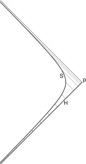
Figure 1: Representation of how the stretched horizon $S$ approximates the past horizon $H$. Note that 2 spatial dimensions are suppressed. Each point in the stretched horizon represents the fluid at constant time $\tau$. As $\alpha\rightarrow 0$, points in the stretched horizon are mapped to points in the past horizon along the ingoing null rays as indicated. A point at infinite $\tau$ is mapped to the bifurcation point $p$.

The fluid itself lives on the spacelike cross section of the stretched horizon defined with the fluid velocity $U^{\mu}$.

Although we have formally identified the stretched horizon system as a “fluid”, one may wonder if this choice has any physical interpretation. Since the stretched horizon is a 2+1 dimensional surface, the fluid must be 2+1 dimensional. In the literature, [21] considered the null vector $l^{\mu}$ associated with null hypersurfaces as an elastic displacement vector of a “spacetime solid” in a long wavelength limit. The entropy of the solid is assumed to be a quadratic functional of derivatives of this vector. When this entropy is maximized gravitational field equations can be obtained. The idea of a fluid living on a lower dimensional surface is also consistent with the hydrodynamic limit of AdS/CFT correspondence. However, there the fluid is taken to be a real gauge theory fluid living on the timelike boundary of AdS spacetime. Is there a real fluid on the stretched horizon here?

We argue that the Minkowski vacuum, which looks like a thermal state when localized into the Rindler wedge of spacetime, obeys the holographic principle [12, 13]. Its properties are encoded into the 2+1 dimensional stretched horizon boundary of the wedge. Some similar ideas can be found in [22]. This appears counterintuitive at first because the vacuum in the Rindler wedge looks like a 3+1 dimensional bath of thermal radiation. However, the entanglement entropy associated with the vacuum is (in the absence of a UV cutoff) a formally divergent quantity that scales like the cross-sectional area of the horizon boundary, not the volume of the wedge. Heuristically, the entropy density of the radiation bath goes like $T^{3}/\hbar^{3}$. The key point is that $T$ is a local Unruh temperature that is a function of the proper length to the horizon: $\sim\hbar\ell^{-1}$. The total entropy is

$$S=\int\ell^{-3}d\ell d^{2}A\sim\delta A~{}\ell_{c}^{-2},$$ (18)

where $\delta A$ is the cross-sectional area of a horizon patch and $\ell_{c}$ is the UV cutoff length. A similar calculation for total energy using density $\sim T^{4}/\hbar^{3}$ also yields an area scaling and stretched horizon energy density $~{}\hbar\ell_{c}^{-3}$. Since these quantities scale like area densities instead of the usual volume densities they will not be extensive unless we identify them with the stretched horizon boundary surface. The degrees of freedom in the vacuum thermal state are effectively packed into the stretched horizon.

Further evidence for this picture is Brustein and Yarom’s work [23] showing that vacuum fluctuations in any sub-volume of Minkowski space scale as the area of the boundary and diverge unless there is a UV cutoff. They used this result to argue that these fluctuations have a representation in terms of a high temperature theory on the boundary, which in the case of the Rindler wedge, is reminiscent of the near-horizon thermal atmosphere with its diverging local temperature. In light of the heuristic arguments above and these results in the literature, we postulate that if hydrodynamical perturbations of the thermal atmosphere exist they should be manifested in the dynamics of a stretched horizon. In particular, in the hydrodynamic limit the degrees of the freedom in the thermal atmosphere can be represented as a real fluid living on the boundary.

3.2 Horizon fluid dynamics

We now examine the dynamics of the horizon fluid in detail. First we discuss the fluid in equilibrium. As in Section 2 around the arbitrary point $p$ in $B$ we can invoke the local flat spacetime approximation to define the local vacuum state. Around this point we have the approximate set of Poincare symmetries, including boosts generated by Killing vector $\chi^{\alpha}$, which is defined to vanish at $p$. Using Rindler coordinates adapted to this boost Killing field $\chi^{\mu}=\frac{\partial}{\partial\tau}$, the metric in the neighborhood of $p$ has the approximate form

$$ds^{2}\approx-\kappa^{2}\rho^{2}d\tau^{2}+d\rho^{2}+dx^{2}+dy^{2}.$$ (19)

The lapse function $\alpha=\kappa\rho$, where $\kappa$ is an arbitrary constant associated with the normalization of boost time $\tau$. In Section 2, $\kappa$ was scaled to be unity and $\tau$ was a dimensionless boost angle. The local Rindler (Killing) horizon at $\alpha=0$ can be approximated by its own stretched horizon for constant $\alpha\rightarrow 0$. The Killing vector $\chi^{\alpha}$ describes the horizon fluid rest frame. However there is the freedom to boost to a moving frame in the $x^{i}\equiv(x,y)$ directions

$$\tau^{\prime} = \gamma(\tau-\beta^{i}x_{i})$$ (20)

$$x^{\prime i} = \gamma(x^{i}-\beta^{i}\tau),$$ (21)

to characterize a moving horizon fluid. In this state the flat spacetime (boosted) Rindler horizon has fixed area and as expected the entropy is unchanging.

Just as in Section 2 we identify the Unruh temperature $\hbar/2\pi\rho=\hbar\kappa/2\pi\alpha$ with the local equilibrium temperature. Notice this has the Tolman law form $\alpha T=T_{0}=\mathrm{const.}$, where $T_{0}=\hbar\kappa/2\pi$ is analogous to a position independent Hawking temperature. In this equilibrium state we expect the fluid is described by a surface stress tensor in the perfect fluid form

$$T^{S}_{\mu\nu}=(\epsilon+P)U_{\mu}U_{\nu}+P\gamma_{\mu\nu}$$ (22)

where $\gamma_{\mu\nu}=g_{\mu\nu}-N_{\mu}N_{\nu}$ and the superscript $S$ indicates this is a surface tensor. Just like entropy density $s$, the surface energy density $\epsilon$ and pressure $P$ are formally divergent quantities that may depend on the number and nature of fields in the thermal atmosphere. We will allow for a UV cutoff length $\ell_{c}$, whose value is initially unknown, which will render all quantities finite. The stretched horizon boundary metric ((19) with $\rho$ fixed) is flat and invariant under translations in time and space. These local translational symmetries in the boundary imply the surface stress tensor is conserved. Using the thermodynamic relations $\epsilon+P=sT$, $d\epsilon=Tds$, and $dP=sdT$ we find the entropy density current

$$\partial_{\mu}(sU^{\mu})=0$$ (23)

is conserved, as expected.

The stretched horizon system of Section 3.1 and the equilibrium fluid do not agree in general: the fluid velocity $U^{\alpha}$ is not proportional to $\chi^{\alpha}$ except as $\tau\rightarrow\infty$ at $x=y=0$. We have chosen this point because in the limit $\alpha\rightarrow 0$, it approaches the bifurcation point at $p$ along the null ray shown in Figure 1. This supplies the notion of local equilibrium in the general fluid. For this non-equilibrium horizon fluid entropy is created externally via heat flux from the outside of the system, and internally from the friction of expansions and shears. This implies the horizon area is not fixed, the entropy current in (23) is not conserved, and the spacetime can no longer be exactly flat. To parameterize the near-horizon curved metric we follow the construction used by [24] to study perturbations of black brane metrics and assume the previously constant $\kappa$ in (19) and boost parameter $\beta^{i}$ in (21) are functions of stretched horizon coordinates $x^{\mu}\equiv(\tau,x,y)$:

$$\kappa \rightarrow \kappa(x^{\mu})$$

$$U^{\mu} = \alpha^{-1}~{}\gamma(x^{\mu})\left(\frac{\partial}{\partial\tau}+\beta^{i}(x^{\mu})\frac{\partial}{\partial x^{i}}\right).$$ (24)

$\kappa(x^{\mu})$ and the boost parameter $\beta^{i}(x^{\mu})$ will approach constant values at $(\infty,0,0)$, where there is no entropy production and the expansion and shear must vanish.

For hydrodynamics to be an applicable description, the horizon gradients $\nabla_{\nu}\ln\kappa$ (or equivalently of $\ln T$) and $\nabla_{\nu}\beta^{i}(x^{\mu})$ (or of $U^{\mu}$) in the local Rindler coordinates need to be $\ll\ell_{\rm{mfp}}^{-1}$ at $(\infty,0,0)$. By dimensional analysis the inverse mean free path of this thermal state is position dependent and $\sim g^{2}T/\hbar$, where $g^{2}$ is an unknown dimensionless parameter.

The gradients and the inverse mean free path are divergent as we approach the true causal horizon $\alpha\rightarrow 0$, but their ratios are finite. The horizon gradient of the local temperature is $\nabla_{\nu}\ln T\sim\alpha^{-1}\nabla_{\nu}\ln\kappa(x^{\mu})$, while Eqn. (17) implies that the gradient has the form

$$\nabla_{\nu}U^{\mu}=\alpha^{-1}\nabla_{\nu}l^{\mu}.$$ (25)

Thus, we need ${\nabla_{\nu}\ln\kappa,\nabla_{\nu}l^{\mu}}\ll g^{2}T_{0}/\hbar\sim\kappa g^{2}$ where now $x^{\mu}=(v,x^{i})$ for horizon Killing time $v$. This criterion is clearly satisfied for derivatives in $v$. This can be seen because the local equilibration time for the system is $\sim g^{-2}\kappa^{-1}$, while the process is assumed to occur for an infinite amount of Killing time before terminating in the equilibrium state. Furthermore in Section 2 there was no requirement on the size of the changes in $x^{i}$ directions of the horizon fluid. The stretched horizon cross-section at $\tau\rightarrow\infty$ (or equivalently the 2-surface $B$ as $\alpha\rightarrow 0$) can be tuned so that the changes in $\beta(x^{i})$ and $\ln\kappa(x^{i})$ are $\ll\kappa g^{2}$ near $p$. Thus, there is no obstruction to working in the hydrodynamic regime and therefore an order by order expansion in derivatives is justified. In the next subsection we will use the equations of hydrodynamics and the properties of stretched horizons to derive the near-equilibrium entropy balance law (9) postulated in Section 2.

3.3 Entropy balance law and vacuum viscosity

Following our above review of hydrodynamics, we can proceed to add a dissipative part to the perfect fluid stress tensor (22) and expand it in derivatives of the flow velocity. Using conservation of the stress tensor in the stretched horizon, the thermodynamic relations $\epsilon+P=sT$, $d\epsilon=Tds$, $dP=sdT$, and making the gauge choice $\Pi_{\mu\nu}U^{\nu}=0$, it follows [20] that entropy balance law for the horizon fluid is

$$\partial_{\mu}(sU^{\mu})=\frac{\delta Q}{T}+\frac{2\eta}{T}\tilde{\sigma}_{\mu\nu}\tilde{\sigma}^{\mu\nu}+\frac{\xi}{T}\tilde{\theta}^{2},$$ (26)

where $\tilde{\sigma}_{\mu\nu}={\textstyle{\frac{1}{2}}}(\nabla_{\mu}U_{\nu}+\nabla_{\nu}U_{\mu}-\theta\gamma_{\mu\nu})$ and $\tilde{\theta}=\nabla_{\gamma}U^{\gamma}$. The Clausius term is the flux of bulk matter energy into the fluid as heat. We will see below that the entropy change on the left hand side of this equation is a finite quantity; the ratios of the divergent quantities on the right hand side will be finite.

Integrating over a volume in the horizon fluid we find

$$\int\partial_{\mu}(sU^{\mu})~{}\alpha d\tau d^{2}A=\frac{2\pi\alpha}{\hbar\kappa}\int\left[T^{M}{}_{\mu\nu}U^{\mu}N^{\nu}\alpha+2\eta\tilde{\sigma}_{\mu\nu}\tilde{\sigma}^{\mu\nu}\alpha+\xi\tilde{\theta}^{2}\alpha\right]d\tau d^{2}A$$ (27)

Using Stokes theorem on the left hand side and then taking the limit $\alpha\rightarrow 0$ along with (17) yields

$$\delta S(v)=\frac{2\pi}{\hbar\kappa}\int\left[T^{M}{}_{\mu\nu}l^{\mu}l^{\nu}+2\eta\hat{\sigma}_{\mu\nu}\hat{\sigma}^{\mu\nu}+\xi\hat{\theta}^{2}\right]dvd^{2}A,$$ (28)

where the $\hat{\sigma}$ and $\hat{\theta}$ are now the expansion and shear of the null $l^{\mu}$. Notice how the $\alpha$’s have also canceled out of the right hand side and the relativistic entropy balance law (27) has been reduced to a non-relativistic form in the true horizon limit, with the left hand side just a change in total entropy in Killing time. This result agrees with the equation for the “long-time” evolution of black hole entropy in the membrane paradigm [11, 25], if we identify $\frac{\hbar\kappa}{2\pi}$ as a Hawking temperature. What is new here is the conceptual picture of (29) as a consequence of relativistic hydrodynamics. This is not present in the Damour-Price-Thorne membrane paradigm because no hydrodynamic limit was identified . Thus, $\eta$ and $\xi$ are not just analogous to viscosities; in our framework it is consistent to identify them as the shear and bulk viscosity of the horizon fluid.

Working with the bifurcation point parameterized as $v=\infty$ is not convenient; therefore we change to the affine parameter $\lambda=-\kappa^{-1}e^{-\kappa v}$ so that $p$ is at the origin: $\lambda=0$ and $x=y=0$. Using the relations $l^{a}=(d\lambda/dv)k^{a}$, $\hat{\theta}=(d\lambda/dv)\theta$, $\hat{\sigma}=(d\lambda/dv)\sigma$, yields

$$\delta S(\lambda)=-\frac{2\pi}{\hbar}\int\left[T^{M}{}_{\mu\nu}k^{\mu}k^{\nu}+2\eta\sigma_{\mu\nu}\sigma^{\mu\nu}+\xi\theta^{2}\right]\lambda~{}d\lambda d^{2}A,$$ (29)

which is consistent with the form of the entropy balance law (9) written in terms of horizon quantities. The matter stress tensor term is the expected flux of boost energy, while the viscous terms form the internal production piece $d_{i}S$. Notice that in general the horizon bulk viscosity $\xi$ also appears in addition to the shear viscosity $\eta$.

We can now proceed to expand the left hand side of (29) order by order in $\lambda$ just as in the original thermodynamic derivation discussed at the end of in Section 2, assuming that the entropy density $s\sim\ell_{c}^{-2}$ is an undetermined quantity such that $\delta S=s\delta A$. At zeroth order the affine expansion at $p$ is again required to be zero. Demanding the linear order equation hold for all null $k^{a}$ and at any arbitrary point $p$ in spacetime, along with local conservation of the bulk matter tensor $\nabla^{\nu}T^{M}{}_{\mu\nu}=0$ yields the Einstein equation and $s$ equal to $(4G_{N}\hbar)^{-1}$. Thus the UV cutoff length is fixed to be $\ell_{c}\sim L_{P}$. The extra shear term in the area change that comes from the Raychaudhuri equation (6) is consistent with the balance law only if the shear viscosity to entropy density is $\eta/s=\hbar/4\pi$, just like in the thermodynamical argument. The bulk viscosity $\xi$ is not determined by the balance law at this order because the affine expansion must be zero at $p$.

4 Discussion

We now conclude with some remarks on the meaning and possible implications of these results. First, to summarize, we argued that the thermodynamic derivation of the Einstein field equations can consistently be reformulated using hydrodynamics. The hydrodynamic degrees of freedom for the local vacuum state are associated with local acceleration horizons through any point. These are closely approximated by surrogate timelike stretched horizons and can be thought of as 2+1 dimensional fluids. The equivalence principle is invoked to view the neighborhood of each point as a piece of flat spacetime with a local Rindler horizon. The entropy of these horizons is fixed and they describe local equilibrium for the horizon fluid. The Unruh effect is then used to effectively assign these equilibrium states a local temperature in the limit where the stretched horizon approaches the true one. On length scales much larger than the mean free path, hydrodynamics must be an accurate description of the physics. When the horizon fluid is out of the equilibrium state, entropy is produced, the horizon area is no longer fixed, and the spacetime can no longer be flat. The entropy balance law is then re-derived using the equations of hydrodynamics. Together with the local conservation of bulk energy-momentum, the balance law implies entropy changes must be governed by the Einstein equation. The Einstein equation thus arises from the hydrodynamics of the local vacuum. Remarkably, this argument also fixes the entropy density and shear viscosity of the vacuum such that their ratio is $\hbar/4\pi$.

Our picture seems to imply that microscopic dynamics (which could include quantum gravity below the cutoff) leads to (semi-)classical Einstein gravity as collective hydrodynamic behavior at low energies. Some ideas in the same spirit can be found in [26]. What is interesting here is that some hydrodynamic properties turn out to be universal although we initially allowed for the properties of the horizon fluid to depend on the number and nature of the quantum fields and treated the viscosities as being purely phenomenological. Once the value of the the UV cutoff scale $\ell_{c}$ was fixed to be roughly a Planck length, the entropy density associated with all local Rindler horizons is the Bekenstein-Hawking entropy density and $\eta/s$ is universally $\hbar/4\pi$. All the dependence on the number and nature of the quantum fields is apparently absorbed into the low energy Newton constant $G_{N}$. This in accord with arguments that the Bekenstein-Hawking entropy is dependent implicitly on the nature of quantum fields through the renormalization of the gravitational constant and is either partly or wholly the entanglement entropy of the thermal atmosphere [27]. These results are puzzling here since no knowledge of microscopic physics was needed to obtain them, only the balance law. We did, on the other hand, fix the value of cutoff scale to be the Planck length “experimentally” by requiring the Einstein equation inferred from the entropy balance law to agree with the observed Einstein equation. Low energy physics (the balance law) and this one observation turn out to be enough to determine the entropy density and the shear viscosity of the fluid. The bulk viscosity though is one fluid property not fixed by the balance law in this case and therefore it seems one would have to know about the details of the microscopic physics in order to determine it.

As we noted in the introduction $\hbar/4\pi$ also appears in the AdS/CFT literature as the universal value of the shear viscosity to entropy density ratio of gauge theories with an Einstein gravity dual. Could this be merely a coincidence or is there a connection between this gauge/gravity duality result and our hydrodynamic derivation? First, in both cases holography is crucial: we postulated the thermal vacuum state is holographic, while AdS/CFT is a precise realization of the equivalence of a higher dimensional gravity theory to a lower dimensional non-gravitational theory on a boundary. Furthermore, in the duality, $d$ dimensional gauge theories in high temperature deconfining phases are dual to large black hole or black brane spacetimes in $d+1$ AdS [28]. Therefore one can use classical perturbations of the large black hole or black brane spacetimes (see [29] for a review) to perform analytical computations of the hydrodynamic transport coefficients. According to the AdS/CFT dictionary the notion of viscosity is meaningful in the infrared regime of the gauge theory, which corresponds to the near horizon limit of the translationally invariant black object. In this sense these black objects have viscosities, just like the viscosity we found for local stretched horizons. In both cases the hydrodynamics of a flat spacetime system is manifested in the dynamics of a horizon boundary. However, since $\hbar/4\pi$ holds for all local acceleration horizons it seems more fundamental than the AdS/CFT results for large black holes and black branes in AdS spacetimes. The dynamics of the local vacuum is governed by gravity itself in the form of Einstein’s equations at each point in an arbitrary spacetime, while the gauge theory dynamics is encoded in the perturbation theory about an AdS gravity background.

In the duality the $\hbar/4\pi$ result holds for both conformal and non-conformal gauge theories. The common feature is strong coupling, in particular very large ’t Hooft coupling. In general the shear viscosity to entropy density ratio of a gauge theory depends on the value of the ’t Hooft coupling [30]. For weakly coupled theories there is a large separation between the mean free path and any other microscopic scale, for example a thermal de Broglie wavelength. In this intermediate region we can use a kinetic theory description where viscosity is due to momentum transfer by quasiparticle motion. Larger mean free paths correspond to an easier momentum transfer and higher viscosity. As the coupling is tuned up the viscosity decreases and the kinetic theory description begins to break down. Nevertheless, extrapolating all the way to strong coupling correctly indicates $\eta/s\sim\hbar$ [29].

This viewpoint suggests the dynamics of the local vacuum thermal state should also be strongly coupled in some sense. In fact, using the results of Section 3.3 we can argue this is the case. From $\eta/s=\hbar/4\pi$, we can roughly determine the other undetermined parameter in our analysis: the dimensionless parameter $g$ in the mean free path. First, from kinetic theory we can estimate $\eta/s\sim\epsilon/s~{}l_{\rm{mfp}}$. Using $\epsilon\sim\hbar\ell_{c}^{-3}$ and $s\sim\ell_{c}^{-2}$ for the thermal state, this implies that

$$\frac{\eta}{s}\sim\hbar\frac{\ell_{\rm{mfp}}}{\ell_{c}}.$$ (30)

Thus, consistency with the entropy balance law implies the mean free path $\ell_{\rm{mfp}}=\frac{\hbar}{g^{2}T}$ is of order the UV cutoff scale $\ell_{c}$. Since $\ell_{c}\sim\hbar/T_{c}$, where $T_{c}$ is the local temperature at the cutoff, we find that $g$ must be roughly of order unity.

We can think of the dimensionless parameter $g^{2}$ in $\eta/s\sim\hbar/g^{2}$ as a coupling which controls the size of the mean free path compared to the microscopic scale (here the UV cutoff scale). If $g^{2}\ll 1$ the mean free path would be much larger than the UV cutoff length and the ratio much larger than $\hbar$. However the hydrodynamic derivation requires $g\sim 1$ and $\ell_{\rm{mfp}}\sim\ell_{c}$, which is indicative of strong coupling.

Typically one would not consider the local vacuum thermal state a strongly coupled system. For example, the vacuum fluctuations of a free field do not appear to be strongly coupled. On the other hand, a free (scalar, for example) field theory in flat spacetime is a continuum field theory and has infinite entanglement entropy. This conflicts with the requirement of a finite entropy and a non-zero cutoff that allowed us to derive the entropy balance law. The balance law implies we must have backreaction effects that distort the flat background spacetime. These gravitational dynamics are imposed up to the UV cutoff, where the physics is strongly coupled. In this regime the entropy density and shear viscosity are universal constants proportional to one another. Since the bulk viscosity is not determined, it may depend on the field content. If this is the case it would be similar to a non-conformal gauge theory, where the bulk viscosity is determined by the mass scales associated with the particular fields that break the conformal symmetry.

Since our picture of the local vacuum thermal state and its dynamics is consistent with key aspects of the gauge/gravity dualities, perhaps it can provide a new perspective on the puzzling aspects of the $\hbar/4\pi$ ratio. For example, although the ratio is derived for relativistic field theories, it is independent of the speed of light $c$ (when we return to cgs dimensions). The hydrodynamic derivation indicates the ratio is tied crucially to the physics of null horizons. As we noticed in (29) the entropy balance law for the local acceleration horizon reduces to a non-relativistic form. The same type of behavior was first noticed in the membrane paradigm [11], where the behavior of a black hole event horizon is analogous to non-relativistic fluid dynamics. Intuitively, the value of the speed of light should not affect the behavior of the intrinsically ultra-relativistic degrees of freedom living on the stretched horizon boundary surface.

An important open question is whether $\hbar/4\pi$ is a universal bound on the shear viscosity to entropy density ratio for all systems, even those that are non-relativistic. Experimental data and the fact that viscosity is larger than $\sim\hbar$ for weakly coupled systems indicate the bound is plausible [16]. It is curious that the conjectured bound is independent of $G_{N}$ even though it is saturated in the special class of theories with a gravity dual. However, in the hydrodynamic derivation we relied only the general thermal properties of the Minkowski vacuum. $G_{N}$ only appears (in the Planck length) when we require agreement with the experiment and fix $\ell_{c}\sim L_{P}$. This indicates that the bound, if it exists, may be a consequence of the behavior of quantum fields when they are localized into regions of flat spacetime. The conjectured bound may also be related to the Bekenstein entropy bound [31], a result also first derived in a gravitational setting, yet which ultimately does not depend on $G_{N}$.

In the future it would be interesting to consider higher curvature corrections to the assumed entropy density and compare the results for the viscosities to the gauge/gravity literature. For example, in the case where the acceleration horizon entropy density is assumed to be a (non-constant, polynomial) function of the Ricci scalar $f(R)$ it was found previously that $\eta/s=\hbar/4\pi$, while the bulk viscosity ratio is $3\hbar f/4\pi$ [8]. Corresponding results in the duality would require study of corrections to non-conformal gauge theories, although an exact comparison is complicated by our inability to determine the bulk viscosity even when an area entropy is assumed. In AdS/CFT, general corrections to Einstein gravity involving contractions of the Ricci and Riemann tensors were found to modify the shear viscosity to entropy density ratio at strong ’t Hooft coupling. With a choice of one parameter the ratio can now be less than $\hbar/4\pi$ [32, 33]. A comparison here would require assuming the local horizon has an entropy density proportional to these contractions and checking the effects in the entropy balance law (29).

Finally, we have only considered linearized hydrodynamics, which was sufficient to derive the Einstein equations and fix the shear viscosity of the local Rindler stretched horizon. However, [24, 34] recently showed the form of the hydrodynamic stress tensor on the AdS boundary is determined up to 2nd order in derivatives by demanding the Einstein equations (with negative cosmological constant) hold for perturbations about black brane spacetimes. The procedure is roughly the inverse of our hydrodynamic derivation: instead of starting with the hydrodynamics of local Rindler stretched horizon and deriving Einstein’s equations, they impose Einstein’s equation order by order in a derivative expansion to derive the stress-tensor at the AdS boundary. The resulting perturbative metrics are dual to solutions of the Navier-Stokes equations. The set of hydrodynamic coefficients at the next order in the stress tensor characterize relaxation times [35, 36]. In our case it would be interesting to see whether higher derivative terms in the stress tensor of the local Rindler stretched horizon can be meaningfully defined and fixed by the entropy balance law.

References

- [1] J. D. Bekenstein, Phys. Rev. D 7, 2333 (1973).
- [2] S. W. Hawking, Commun. Math. Phys. 43, 199 (1975) [Erratum-ibid. 46, 206 (1976)].
- [3] T. Jacobson, Phys. Rev. Lett. 75, 1260 (1995) [arXiv:gr-qc/9504004].
- [4] J. J. Bisognano and E. H. Wichmann, J. Math. Phys. 16, 985 (1975).
- [5] W. G. Unruh and N. Weiss, Phys. Rev. D 29, 1656 (1984).
- [6] T. Padmanabhan, Class. Quant. Grav. 19, 5387 (2002) [arXiv:gr-qc/0204019]; A. Paranjape, S. Sarkar and T. Padmanabhan, Phys. Rev. D 74, 104015 (2006) [arXiv:hep-th/0607240]; D. Kothawala, S. Sarkar and T. Padmanabhan, Phys. Lett. B 652, 338 (2007) [arXiv:gr-qc/0701002].
- [7] M. Akbar and R. G. Cai, Phys. Rev. D 75, 084003 (2007) [arXiv:hep-th/0609128].
- [8] C. Eling, R. Guedens and T. Jacobson, Phys. Rev. Lett. 96, 121301 (2006) [arXiv:gr-qc/0602001].
- [9] E. Elizalde and P. J. Silva, arXiv:0804.3721 [hep-th].
- [10] T. Damour, these de doctorat d’etat, University of Paris VI, (1979) (unpublished); T. Damour, in Proceedings of the Second Marcel Grossmann Meeting on General Relativity, edited by R. Ruffini (North-Holland, Amsterdam, 1982), p. 587.
- [11] R. H. Price and K. S Thorne, Phys. Rev. D 33, 915 (1986); Black Holes: The Membrane Paradigm, edited by K. S. Thorne, R. H. Price, and D. A. MacDonald (Yale University Press, London, 1986); M. Parikh and F. Wilczek, Phys. Rev. D 58, 064011 (1998) [arXiv:gr-qc/9712077].
- [12] G. ’t Hooft, in Abdus Salam Festschrift: A Collection of Talks, edited by A. Aly, J. Ellis, and S. Randjbar-Daemi (World Scientific, Singapore, 1993) [arXiv:gr-qc/9310026].
- [13] L. Susskind, J. Math. Phys. 36, 6377 (1995) [arXiv:hep-th/9409089].
- [14] J. M. Maldacena, Adv. Theor. Math. Phys. 2, 231 (1998) [Int. J. Theor. Phys. 38, 1113 (1999)] [arXiv:hep-th/9711200]; O. Aharony, S. S. Gubser, J. M. Maldacena, H. Ooguri and Y. Oz, Phys. Rept. 323, 183 (2000) [arXiv:hep-th/9905111].
- [15] P. Kovtun, D. T. Son and A. O. Starinets, JHEP 0310, 064 (2003) [arXiv:hep-th/0309213]; A. Buchel and J. T. Liu, Phys. Rev. Lett. 93, 090602 (2004) [arXiv:hep-th/0311175].
- [16] P. Kovtun, D. T. Son and A. O. Starinets, Phys. Rev. Lett. 94, 111601 (2005) [arXiv:hep-th/0405231].
- [17] T. D. Cohen, Phys. Rev. Lett. 99, 021602 (2007) [arXiv:hep-th/0702136]; A. Cherman, T. D. Cohen and P. M. Hohler, JHEP 0802, 026 (2008) [arXiv:0708.4201 [hep-th]]; D. T. Son, Phys. Rev. Lett. 100, 029101 (2008) [arXiv:0709.4651 [hep-th]]; T. D. Cohen, arXiv:0711.2664 [hep-th].
- [18] L. Bombelli, R. K. Koul, J. H. Lee and R. D. Sorkin, Phys. Rev. D 34, 373 (1986); M. Srednicki, Phys. Rev. Lett. 71, 666 (1993) [arXiv:hep-th/9303048].
- [19] S. R. de Groot and P. Mazur, Non-Equilibrium Thermodynamics, (North-Holland, 1962).
- [20] L. D. Landau and E. M. Lifshitz, Fluid Mechanics (Pergamon Press, 1987).
- [21] T. Padmanabhan, Int. J. Mod. Phys. D 13, 2293 (2004) [arXiv:gr-qc/0408051]; T. Padmanabhan and A. Paranjape, Phys. Rev. D 75, 064004 (2007) [arXiv:gr-qc/0701003] and references therein.
- [22] for ideas on Rindler horizon holography using action functionals, see A. Mukhopadhyay and T. Padmanabhan, Phys. Rev. D 74, 124023 (2006) [arXiv:hep-th/0608120]; T. Padmanabhan, AIP Conf. Proc. 939, 114 (2007) [arXiv:0706.1654 [gr-qc]] and references therein.
- [23] R. Brustein and A. Yarom, JHEP 0501, 046 (2005) [arXiv:hep-th/0302186]; R. Brustein and A. Yarom, Phys. Rev. D 69, 064013 (2004) [arXiv:hep-th/0311029] and references therin.
- [24] S. Bhattacharyya, V. E. Hubeny, S. Minwalla and M. Rangamani, JHEP 0802, 045 (2008) [arXiv:0712.2456 [hep-th]].
- [25] B. Carter, in General Relativity, An Einstein Centenary Survey, ed. S. W. Hawking and W. Israel (Cambridge Univ. Press, 1979), 294.
- [26] see, for example G. Volovik, arXiv:gr-qc/0612134; G. Volovik, The Universe in a Helium Droplet (Clarendon Press, Oxford, 2003) and references therein
- [27] L. Susskind and J. Uglum, Phys. Rev. D 50, 2700 (1994) [arXiv:hep-th/9401070]; T. Jacobson, arXiv:gr-qc/9404039; S. N. Solodukhin, [arXiv:hep-th/9504022]; F. Larsen and F. Wilczek, Nucl. Phys. B 458, 249 (1996) [arXiv:hep-th/9506066].
- [28] E. Witten, Adv. Theor. Math. Phys. 2, 505 (1998) [arXiv:hep-th/9803131].
- [29] D. T. Son and A. O. Starinets, Ann. Rev. Nucl. Part. Sci. 57, 95 (2007) [arXiv:0704.0240 [hep-th]].
- [30] A. Buchel, J. T. Liu and A. O. Starinets, Nucl. Phys. B 707, 56 (2005) [arXiv:hep-th/0406264]; R. C. Myers, M. F. Paulos and A. Sinha, arXiv:0806.2156 [hep-th].
- [31] J. D. Bekenstein, Phys. Rev. D 23, 287 (1981).
- [32] M. Brigante, H. Liu, R. C. Myers, S. Shenker and S. Yaida, Phys. Rev. D 77, 126006 (2008) [arXiv:0712.0805 [hep-th]].
- [33] Y. Kats and P. Petrov, arXiv:0712.0743 [hep-th].
- [34] R. Baier, P. Romatschke, D. T. Son, A. O. Starinets and M. A. Stephanov, JHEP 0804, 100 (2008) [arXiv:0712.2451 [hep-th]]
- [35] W. Israel and J. M. Stewart, Annals Phys. 118, 341 (1979)
- [36] M. P. Heller and R. A. Janik, Phys. Rev. D 76, 025027 (2007) [arXiv:hep-th/0703243]; M. Natsuume and T. Okamura, Phys. Rev. D 77, 066014 (2008) [arXiv:0712.2916 [hep-th]].