Multi-instanton and String Loop Corrections in Toroidal Orbifold Models

CPHT-RR040.0608
LPT-ORSAY 08-57

We analyze $\mathcal{N}=2$ (perturbative and non-perturbative) corrections to the effective theory in type I orbifold models where a dual heterotic description is available. These corrections may play an important role in phenomenological scenarios. More precisely, we consider two particular compactifications: the Bianchi-Sagnotti-Gimon-Polchinski orbifold and a freely-acting $\mathbb{Z}_{2}\times\mathbb{Z}_{2}$ orbifold with $\mathcal{N}=1$ supersymmetry and gauge group $SO(q)\times SO(32-q)$. By exploiting perturbative calculations of the physical gauge couplings on the heterotic side, we obtain multi-instanton and one-loop string corrections to the Kähler potential and the gauge kinetic function for these models. The non-perturbative corrections appear as sums over relevant Hecke operators, whereas the one-loop correction to the Kähler potential matches the expression proposed in [1, 2]. We argue that these corrections are universal in a given class of models where target-space modular invariance (or a subgroup of it) holds.

1 Introduction

In the last years there has been a remarkable progress in understanding the structure of String Theory at tree-level in the perturbative expansion, that is, in the supergravity limit. Flux compactifications [3] have provided us with a helpful framework which partially addresses long-standing problems such as moduli stabilization or supersymmetry breaking. However, despite this progress, the resulting message continues to be that non-perturbative and string loop corrections play an indispensable role, mainly due to the generic presence of remnant flat directions in the scalar potential and the difficulties of obtaining a chiral spectrum in their absence.

The computation of $\alpha^{\prime}$ and non-perturbative corrections to the effective theory is still in an early stage, even for cases where a description in terms of a free CFT is available. Much effort has been pursued on understanding the role of $\mathcal{N}=1$ euclidean brane instantons [4]. These may turn out to be useful for generating new couplings in the superpotential [5, 6, 7, 8, 9], moduli-stabilization [10] or supersymmetry breaking [11]. Moreover, the one-loop string corrections to the Kähler potential computed in [12], have been shown to play an important role in large volume scenarios [13], leading to a hierarchy of mass scales without the necessity of a big amount of fine-tuning. Additional one-loop string corrections to the Kähler potential have been computed in [1, 2] for toroidal compactifications (see also [14, 15]).

In this note, we analyze multi-instanton and one-loop string corrections arising from $\mathcal{N}=2$ sectors in toroidal orbifold compactifications of type I String Theory. These generically correct the Kähler potential, $K$, and the gauge kinetic function, $f_{a}$, of the effective theory, and therefore may play an important role in phenomenological scenarios with classical flat directions. For this aim, we follow the techniques introduced in [16], and build type I-heterotic S-dual pairs of orbifold models.

Schematically, the procedure can be summarized as follows. The one-loop physical gauge couplings in the heterotic side take the expression,

$$4\pi^{2}g_{a}^{-2}(\mu^{2})|_{\rm 1-loop}=\frac{k_{a}}{\ell}+\frac{b_{a}}{4}\textrm{log}\frac{M_{\rm s}^{2}}{\mu^{2}}+\frac{\Delta_{a}(M,\bar{M})}{4}\ ,$$ (1)

with $\ell$ the linear multiplet associated to the dilaton, $M_{s}$ the string scale, $M$ the moduli of the compactification and $k_{a}$ the normalization of the gauge group generators, determined by the level of the corresponding Kac-Moody algebra. The $\beta$-function coefficient, $b_{a}$, is given in terms of the quadratic Casimir invariants of the gauge group,

$$b_{a}=\sum_{r}n_{r}T_{a}(r)-3T_{a}({\rm adj}_{a})\ ,$$ (2)

with $n_{r}$ the number of matter multiplets in the representation $r$.

On the other hand, the field theory result reads [17, 18],

$$4\pi^{2}g_{a}^{-2}(\mu^{2})|_{\rm 1-loop}=\textrm{Re }f_{a}(M)|_{\rm 1-loop}+\frac{b_{a}}{4}\left(\textrm{log}\frac{M_{\rm Planck}^{2}}{\mu^{2}}-\textrm{log}(S+\bar{S})\right)+\\ +\frac{1}{4}\left(c_{a}\hat{K}(M,\bar{M})-2\sum_{r}T_{a}(r)\textrm{log det }Z_{r}(M,\bar{M})\right)\ ,$$ (3)

where det $Z_{r}$ is the determinant of the tree-level Kähler metric associated to the matter multiplets in the representation $r$, $\hat{K}(M,\bar{M})$ the tree-level Kähler potential for the moduli $M$ and,

$$c_{a}=\sum_{r}n_{r}T_{a}(r)-T({\rm adj}_{a})\ .$$ (4)

In order to compare (1) and (3), it is convenient to express the relation between the usual complex axiodilaton $S$ and the linear multiplet $\ell$ as,

$$\frac{1}{\ell}=\textrm{Re }S-\frac{1}{4}\Delta_{\textrm{univ.}}$$ (5)

with $\Delta_{\textrm{univ.}}$ a gauge group independent (“universal”) function. In what follows we split $\Delta_{\textrm{univ.}}$ in its harmonic and non-harmonic parts,

$$\Delta_{\textrm{univ.}}(M,\bar{M})=V_{(1)}(M,\bar{M})+H(M)+H^{*}(\bar{M})\ .$$ (6)

In terms of these, the Kähler potential and the gauge-kinetic function of the $\mathcal{N}=1$ effective theory are given to one-loop by [19, 18, 20],

$$K|_{\rm 1-loop} =-\textrm{log}\left(S+\bar{S}-\frac{1}{2}V_{(1)}(M,\bar{M})\right)+\hat{K}(M,\bar{M})\ ,$$ (7)

$$\textrm{Re }f_{a}|_{\rm 1-loop} =k_{a}\textrm{Re }S+\frac{1}{4}\left(\Delta_{a}(M,\bar{M})-V_{(1)}(M,\bar{M})-c_{a}\hat{K}(M,\bar{M})\right.$$

$$\left.\qquad\qquad\qquad\qquad\qquad\qquad-2\sum_{r}T_{a}(r)\textrm{log det }Z_{r}(M,\bar{M})\right)$$ (8)

We can then reinterpret the results in terms of $E1$ multi-instanton and string loop corrections on the type I side, as $K$ and $f_{a}$ should be invariant (up to Kähler transformations) under S-duality transformations.

In the present work, we consider in detail two classes of models on which the heterotic S-dual partition function can be easily worked out: the Bianchi-Sagnotti-Gimon-Polchinsky (BSGP) orbifold [21, 22], with gauge group $U(16)\times U(16)$, and the $\mathbb{Z}_{2}\times\mathbb{Z}_{2}$ freely-acting orbifold model with gauge group $SO(q)\times SO(32-q)$, presented in [16] and based on the model of [23] (see also [24]). The motivation is multiple. First, based on the modular symmetries preserved by the scalars in Calabi-Yau compactifications, and more precisely on the axionic shift symmetries, it has been argued in [25] that non-perturbative corrections to the gauge kinetic function should appear in an exponentiated form, $\textrm{exp}(2\pi M)$, with $M$ the corresponding moduli. Our results on the BSGP orbifold show indeed that global symmetries constrains very much the shape of multi-instanton and string-loop corrections and, with few extra assumptions, they are completely determined in models on which modular invariance in the moduli space of the compactification applies.

The freely-acting $SO(q)\times SO(32-q)$ orbifold model represents, on the other hand, an example on which part of the original modular symmetry is broken by the compactification. A remarkable fact, already pointed out in [16], is that $E1$ instantons in this model always appear within multiplets under the orbifold action (doublets or quadruplets). We believe that this may be a general feature of flux compactifications, where the fluxes gauge some of the original symmetries and induce non-trivial discrete torsion. It is therefore interesting to see how non-perturbative and loop corrections are affected by the “background” in this simple example. Moreover, it was also observed in [16] that, in the heterotic S-duals, the orbifold action on the winding modes was different for $q=0$ (mod 8) or $q=4$ (mod 4), pointing out a possible dependence of the type I instantonic effects on the rank of the gauge group. It is also our aim to make this dependence explicit.

Although similar computations to the ones performed here have been carried out e.g. for $R^{4}$ [26, 27], $F^{4}$ [29, 30, 27, 31] and the four hyperini [32] couplings, this is to our knowledge the first explicit computation of stringy multi-instanton corrections to the Kähler potential and the gauge kinetic function. We hope that these results will help to shed some light on some of the issues raised in the previous paragraphs, and more interestingly, to clarify the possible role of these corrections in phenomenological scenarios.

The paper is organized as follows. In section 2 we construct the partition function for the heterotic S-dual of the BSGP orbifold model, and extract the $E1$ multi-instanton and one-loop string corrections to the Kähler potential and the gauge kinetic function in the resulting effective theory. In section 3 we proceed similarly with the $SO(q)\times SO(32-q)$ freely acting orbifold model. We comment on the possible “universality” of some of our results and discuss about possible generalizations in section 4. Finally, we give some concluding remarks in section 5. We have relegated all the details on the computations to the appendix, in order not to overload the bulk of the paper with many technicalities.

2 The Bianchi-Sagnotti-Gimon-Polchinski orbifold

In this section we consider the BSGP type I orbifold model [21, 22], corresponding to the $T^{4}/\mathbb{Z}_{2}\times T^{2}$ orbifold limit of type I String Theory compactified in $K3\times T^{2}$. In order to cancel the RR tadpoles, 8 D5-branes and 16 D9-branes are required. For D5 branes lying on top of an orbifold fixed point, the complete massless spectrum has a $U(16)\times U(16)$ gauge group with hypermultiplets in $2(\mathbf{120},\mathbf{1})+2(\mathbf{1},\mathbf{120})+(\mathbf{16},\mathbf{16})$. In the Coulomb branch, where half D5-brane is located at each of the 16 fixed points, the Green-Schwarz mechanism takes place and only the $U(16)$ gauge group from the D9-branes remains massless, with spectrum given by four hypermultiplets, containing the moduli of the $K3$, three vector multiplets containing the axiodilaton and the moduli of the $T^{2}$, a $\mathbf{120}+\overline{\mathbf{120}}$, and sixteen $\mathbf{16}$ coming from the D5-D9 modes. The coefficient of the $\beta$-function turns out to be $b_{U(16)}=12$. Perturbative threshold corrections to gauge couplings [38] depend on the moduli of $T^{2}$, denoted $T_{1}$ and $U_{1}$ in what follows. Since the dilaton $S$ and $T_{1},U_{1}$ are in ${\cal N}=2$ vector multiplets in 4d language, this is consistent with supersymmetry. A priori we expect non-perturbative corrections to depend nontrivially on the three vector multiplets, and to be insensitive to the $T^{4}/\mathbb{Z}_{2}$ moduli, called $T_{2,3}$ and $U_{2,3}$ in what follows. We will show, by performing explicitly the computation using the heterotic S-dual, that this expectation is indeed correct.

2.1 Heterotic S-dual partition function

We want to find the one-loop partition function for the heterotic dual of the BSGP model, proposed in [39] for the above Coulomb branch. In [40] it was shown that this corresponds to a standard $SO(32)$ heterotic $T^{2}\times T^{4}/\mathbb{Z}_{2}$ orbifold with shift vector $V=\frac{1}{4}(1,\ldots,1,-3)$. The various orbifold blocks are then as follows. The left-moving fermions contribute as,

$$Z_{\textrm{L}}\left[{h\atop g}\right]=\frac{1}{2\eta^{4}}\sum_{a,b=0}^{1}(-1)^{a+b+ab+bh}\vartheta^{2}\left[{a\atop b}\right]\vartheta^{2}\left[{a+h\atop b+g}\right]\ ,$$ (9)

with $h,g=0,1$ labelling the different untwisted and twisted orbifold sectors.

Analogously, the bosonic $T^{4}$ blocks read,

$$Z_{(4,4)}\left[{0\atop 0}\right]=\frac{\hat{Z}_{2}\hat{Z}_{3}}{|\eta|^{8}}\quad\textrm{and}\quad Z_{(4,4)}\left[{h\atop g}\right]=\left|\frac{2\eta}{\vartheta\left[{1-h\atop 1-g}\right]}\right|^{4}\ ,\quad\textrm{for }hg\neq 0\ .$$ (10)

Here we have defined the toroidal lattice sums $\hat{Z}_{r}$ as,

$$\hat{Z}_{r}=\frac{\textrm{Re }T_{r}}{\tau_{2}}\sum_{n_{1},\ell_{1},n_{2},\ell_{2}}\textrm{exp}\left[-2\pi T_{r}\textrm{det}(A)-\frac{\pi(\textrm{Re }T_{r})}{\tau_{2}(\textrm{Re }U_{r})}\left|\begin{pmatrix}1&iU_{r}\end{pmatrix}A\begin{pmatrix}\tau\\ -1\end{pmatrix}\right|^{2}\right]\ ,$$ (11)

$$A=\begin{pmatrix}n_{1}&\ell_{1}\\ n_{2}&\ell_{2}\end{pmatrix}\ ,$$ (12)

with $n_{i}$ and $\ell_{i}$ integers. For the right moving fermions we find,

$$\Gamma\left[{h\atop g}\right]=\frac{1}{2\bar{\eta}^{16}}\sum_{a,b=0}^{1}(-1)^{ga+hb}e^{-\frac{i\pi hg}{2}}\bar{\vartheta}^{16}\left[{a-\frac{h}{2}\atop b-\frac{g}{2}}\right]\ .$$ (13)

Putting everything together we finally get the one-loop partition function for the heterotic dual of the BSGP model,

$$T=\int_{\mathcal{F}}\frac{d^{2}\tau}{\tau_{2}^{3}}\frac{\hat{Z}_{1}}{4|\eta|^{8}}\left[(Q_{o}+Q_{v})\frac{\hat{Z}_{2}\hat{Z}_{3}}{|\eta|^{8}}\Gamma\left[{0\atop 0}\right]+(Q_{o}-Q_{v})\left|\frac{2\eta}{\vartheta_{2}}\right|^{4}\Gamma\left[{0\atop 1}\right]\right.+\\ \left.+(Q_{s}+Q_{c})\left|\frac{2\eta}{\vartheta_{4}}\right|^{4}\Gamma\left[{1\atop 0}\right]+(Q_{s}-Q_{c})\left|\frac{2\eta}{\vartheta_{3}}\right|^{4}\Gamma\left[{1\atop 1}\right]\right]\ ,$$ (14)

where,

$$Q_{o}+Q_{v} =\frac{1}{2\eta^{4}}(\vartheta_{3}^{4}-\vartheta_{1}^{4}-\vartheta_{2}^{4}-\vartheta_{4}^{4})\ ,$$ (15)

$$Q_{o}-Q_{v} =\frac{1}{2\eta^{4}}(\vartheta_{3}^{2}\vartheta_{4}^{2}-\vartheta_{4}^{2}\vartheta_{3}^{2}-\vartheta_{1}^{2}\vartheta_{2}^{2}-\vartheta_{2}^{2}\vartheta_{1}^{2})\ ,$$ (16)

$$Q_{s}-Q_{c} =\frac{1}{2\eta^{4}}(\vartheta_{1}^{2}\vartheta_{3}^{2}+\vartheta_{3}^{2}\vartheta_{1}^{2}+\vartheta_{4}^{2}\vartheta_{2}^{2}-\vartheta_{2}^{2}\vartheta_{4}^{2})\ ,$$ (17)

$$Q_{s}+Q_{c} =\frac{1}{2\eta^{4}}(\vartheta_{3}^{2}\vartheta_{2}^{2}-\vartheta_{2}^{2}\vartheta_{3}^{2}+\vartheta_{4}^{2}\vartheta_{1}^{2}+\vartheta_{1}^{2}\vartheta_{4}^{2})\ .$$ (18)

2.2 Perturbative and non-perturbative corrections

Following the general discussion around (1), our task here is to compute the one-loop threshold corrections to the physical gauge coupling in the heterotic model (14), as these are mapped to one-loop and $E1$ multi-instanton corrections in the BSGP orbifold. In terms of the partition function, these are given by [33, 34, 35],

$$\Lambda\equiv\frac{b_{U(16)}}{4}\textrm{log}\frac{M_{\rm s}^{2}}{\mu^{2}}+\frac{\Delta_{U(16)}}{4}=\int_{\mathcal{F}}\frac{d^{2}\tau}{\tau_{2}}\frac{i}{4\pi}\frac{1}{|\eta|^{4}}\sum_{a,b=0}^{1}\partial_{\tau}\left(\frac{\vartheta\left[{a\atop b}\right]}{\eta}\right)\left(Q^{2}-\frac{1}{4\pi\tau_{2}}\right)C\left[{a\atop b}\right]\ ,$$ (19)

where $Q$ is the charge operator of the corresponding gauge group, and $C\left[{a\atop b}\right]$ is the internal six-dimensional partition function. Following the same procedure than in [16] we find,

$$\Lambda=-\frac{1}{8}\int_{\mathcal{F}}\frac{d^{2}\tau}{\tau_{2}}\hat{Z}_{1}\hat{\mathcal{A}}_{f}$$ (20)

with,

$$\hat{\mathcal{A}}_{f}=-\frac{1}{20\eta^{24}}(D_{10}E_{10}-48\eta^{24})=\frac{1}{12\eta^{24}}\left(\hat{E}_{2}E_{4}E_{6}-\frac{5}{12}E_{6}^{2}-\frac{7}{12}E_{4}^{3}\right)\ ,$$ (21)

and $\hat{Z}_{1}$ given in (11). The definitions of the Eisenstein series, $E_{2k}$, can be found for instance in the appendix of [16].

The details of the computation are in appendix A.1. Notice that the numerator of $\hat{\mathcal{A}_{f}}$ is an almost-holomorphic modular form, their non-holomorphicity being exclusively due to the presence of $\hat{E}_{2}$,

$$\hat{E}_{2}\equiv E_{2}-\frac{3}{\pi\tau_{2}}\ .$$ (22)

As it will be made more explicit below, these non-holomorphic terms can be traced back to perturbative and non-perturbative corrections to the Kähler potential of the effective theory.

Both, $\hat{Z}_{1}$ and $\hat{\mathcal{A}}_{f}$, are invariant under the full modular group $\Gamma$, so we can directly apply the method of Dixon-Kaplunovsky-Louis (DKL) [34] to evaluate the integral in (20). This consists on depicting the lattice sum, $\hat{Z}_{1}$, into orbits under the modular group, and evaluate the integral for each class of orbits in a suitable unfolded region of the upper complex half-plane. The matrices (12) can be classified in three kind of orbits under the modular group,

1. Zero orbit:

   $$\begin{pmatrix}0&0\\ 0&0\end{pmatrix}\ ,$$

2. Non-degenerate orbits:

   $$\begin{pmatrix}k&j\\ 0&p\end{pmatrix}\ ,$$

   with $k>j\geq 0$, $p\neq 0$ and $AV=AV^{\prime}$ iff $V=V^{\prime}$, for $V,V^{\prime}\in\Gamma$.

3. Degenerate orbits:

   $$\begin{pmatrix}0&j\\ 0&p\end{pmatrix}\ ,$$

   with $(j,p)\sim(-j,-p)$ and $AV=AV^{\prime}$ iff $V=T^{n}V^{\prime}$, for some integer $n$ and $V,V^{\prime}\in\Gamma$.

We therefore unfold (20) into three integrals corresponding to the above representatives. Non-degenerate orbits are integrated over the double cover of the upper half complex plane, $\mathbb{C}^{+}$, whereas degenerate orbits have to be integrated over the fundamental domain, $\mathcal{F}_{T}$, of the subgroup generated by $T$, for arbitrary $j$ and $p$. The details of the computation can be found in appendix A.1. Putting all pieces together and disregarding constant terms arising from the regularization scheme, we obtain,

$$\Lambda=\frac{\pi}{2}\textrm{Re }T_{1}\ -\ 3\left(\textrm{log}|\eta(iU_{1})|^{4}+\textrm{log}[(\textrm{Re }U_{1})(\textrm{Re }T_{1})\mu^{2}]\right)\ -\ \frac{\pi}{3}\frac{E(iU_{1},2)}{T_{1}+\bar{T}_{1}}-\\ -\frac{1}{4}\left(\sum_{k>j\geq 0,p>0}\frac{1}{kp}e^{-2\pi pkT_{1}}\left[\hat{\mathcal{A}}_{f}(\mathcal{U})+\frac{1}{\pi kp}\frac{\hat{\mathcal{A}}_{K}(\mathcal{U})}{T_{1}+\bar{T}_{1}}\right]\ +\ \textrm{c.c.}\right)$$ (23)

where $E(U,k)$ is the non-holomorphic Eisenstein series of order $k$, defined as

$$E(U,k)\equiv\frac{1}{\zeta(2k)}\sum_{(j_{1},j_{2})\neq(0,0)}\frac{(\textrm{Im }U)^{k}}{|j_{1}+j_{2}U|^{2k}}\ ,$$ (24)

and $\hat{\mathcal{A}}_{K}$ the almost-holomorphic modular form,

$$\hat{\mathcal{A}}_{K}=\frac{1}{12\eta^{24}}(\hat{E}_{2}E_{4}E_{6}+2E_{6}^{2}+3E_{4}^{3})\ .$$ (25)

The second term in (23) matches precisely the one-loop threshold corrections computed in [38], whereas the second line in (23), corresponds to $E1$ multi-instanton corrections. These are wrapping the first 2-torus, with induced worldvolume complex structure [29],

$$\mathcal{U}=\frac{j+ipU_{1}}{k}\ ,$$ (26)

as depicted in figure 1.

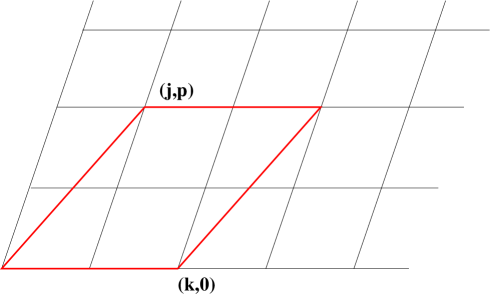
Figure 1: E1 multi-instanton wrapping the first 2-torus, with induced worldvolume complex structure $\mathcal{U}$ given in (26).

Their contribution can be also expressed as a sum over standard Hecke operators acting on (almost-holomorphic) modular invariant forms,

$$\sum_{k>j\geq 0,p>0}\frac{1}{kp}e^{-2\pi pkT_{1}}\left[\hat{\mathcal{A}}_{f}(\mathcal{U})+\frac{1}{\pi kp}\frac{\hat{\mathcal{A}}_{K}(\mathcal{U})}{T_{1}+\bar{T}_{1}}\right]=\\ \sum_{N=1}^{\infty}e^{-2\pi NT_{1}}H_{N}\left[\hat{\mathcal{A}}_{f}+\frac{1}{N\pi}\frac{\hat{\mathcal{A}}_{K}}{T_{1}+\bar{T}_{1}}\right](iU_{1})$$ (27)

with,

$$H_{N}[\Phi](iU)=\frac{1}{N}\sum_{p>0,\ kp=N}\sum_{k>j\geq 0}\Phi\left(\frac{j+ipU}{k}\right)\ .$$ (28)

It is thus evident the invariance of (23) under $SL(2,\mathbb{Z})$ transformations of $U_{1}$, in agreement with the global symmetry preserved by the orbifold.

In order to extract from (23) the corrections to the effective theory, we need the Kähler metric for the D9-D9 and D9-D5 matter fields. This is given by [52, 53],

$$K_{C_{k}^{99}\bar{C}_{k}^{99}}=\frac{1}{(T_{k}+\bar{T}_{k})(U_{k}+\bar{U}_{k})}\ ,\qquad K_{C_{k}^{95}\bar{C}_{k}^{95}}=\prod_{j=2,3}\frac{1}{[(T_{j}+\bar{T}_{j})(U_{j}+\bar{U}_{j})]^{1/2}}\ ,$$ (29)

for $k=1,2,3$, so that,

$$\sum_{r}T_{a}(r)\textrm{log det }Z_{r}(M,\bar{M})=\\ -16\ \textrm{log}[(T_{1}+\bar{T}_{1})(U_{1}+\bar{U}_{1})]-22\sum_{j=2,3}\textrm{log}[(T_{j}+\bar{T}_{j})(U_{j}+\bar{U}_{j})]\ .$$ (30)

From (7) and (8), then we read the following expressions for the corrected Kähler potential and gauge kinetic function in the effective theory,

$$K=-\textrm{log}(S+\bar{S})-\sum_{i=1}^{3}\textrm{log}[(T_{i}+\bar{T}_{i})(U_{i}+\bar{U}_{i})]+\frac{1}{2}\frac{V_{1-loop}+V_{E1}}{S+\bar{S}}\ ,$$ (31)

$$V_{1-loop}=-\frac{4\pi}{3}\frac{E(iU_{1},2)}{T_{1}+\bar{T}_{1}}\ ,$$ (32)

$$V_{E1}=-\frac{1}{\pi}\sum_{k>j\geq 0,\ p>0}\frac{e^{-2\pi kpT_{1}}}{(kp)^{2}}\left[\frac{\hat{\mathcal{A}}_{K}(\mathcal{U})}{T_{1}+\bar{T}_{1}}-\frac{2ikp}{\mathcal{U}-\bar{\mathcal{U}}}\frac{E_{10}(\mathcal{U})}{\eta^{24}(\mathcal{U})}\right]\ +\ \textrm{c.c.}\ ,$$ (33)

$$f_{U(16)}=S+\frac{\pi T_{1}}{2}-12\textrm{log }\eta(iU_{1})-\frac{1}{2}\sum_{k>j\geq 0,\ p>0}\frac{e^{-2\pi kpT_{1}}}{kp}\mathcal{A}_{f}(\mathcal{U})\ ,$$ (34)

where the holomorphic modular form $\mathcal{A}_{f}$ is defined as in (21), replacing $\hat{E}_{2}$ by $E_{2}$. Several comments are in order. First, observe that the $\beta$-function coefficient exactly matches the field theory result. Moreover, the one-loop $\alpha^{\prime}$ correction to the Kähler potential agrees with the expression obtained in [1, 2] by direct computation in the type I side. In our context, these corrections come from non-holomorphic terms in the contributions of degenerate orbits. Modular transformations of the $T_{1}$ modulus mix the $\alpha^{\prime}$ corrections with the instantonic terms, in agreement with the fact that T-duality is not a symmetry of type I String Theory. Notice also that the loop correction of [12], proportional to $(\textrm{Re }S)^{3/2}$, is missing. This is consistent with the fact that the internal torus has zero Euler characteristic, $\chi=0$, for which the coefficient in front of the above correction vanishes.

From the field theory perspective, the E1 multi-instanton corrections of eq.(27), enter as corrections to both the Kähler potential and the holomorphic gauge kinetic function. To our knowledge, these are new corrections and their role in the low energy effective theory still has to be clarified. In section 4, we will argue that these non-perturbative corrections are general for any $\mathcal{N}=2$ sector in orbifold compactifications where modular invariance of the target-space holds.

Finally, the presence of the first term in the heterotic threshold correction (23), contributing to the gauge kinetic function (34), may seem puzzling at first sight. Indeed, by a straightforward counting of the string coupling, this linear term in the $T^{2}$ volume modulus $T_{1}$, is expected to be a tree-level (disk) effect on the type I side. On the other hand, the $T_{1}$ modulus in the type I $\mathbb{Z}_{2}$ orbifold couples at tree-level only to type I D5 branes. A possible origin is the following. D9-branes in the BSGP model are fractional and therefore its gauge kinetic function should receive a contribution proportional to,

$$\sim\ \sum\sqrt{\textrm{det}(P[G+F_{2}])}\ T_{1}\ ,$$ (35)

where the sum runs over the 16 singularities of $T^{4}/\mathbb{Z}_{2}$ and $P[\ldots]$ is the pull-back to the collapsed 2-cycle of the singularity. In the orbifold limit, the volume of the 2-cycle is zero and therefore the contribution from the metric vanishes. However, as pointed out in [39], there is a non-trivial U(1) gauge bundle on the collapsed 2-cycles which, in the blow-up limit, leads together with the 8 D5-branes to the 24 instantons which are required to satisfy RR 3-form Bianchi identity, $dF_{3}=\textrm{Tr }R\wedge R-\textrm{Tr }F_{2}\wedge F_{2}$, in a smooth K3. It is therefore expected a linear contribution to the gauge kinetic function of the D9-brane from this hidden U(1) bundle at the singularities.

2.3 $E1$ instantons

Type I String Theory and its toroidal orbifolds has E5 instantons wrapping the whole internal space and E1 instantons wrapping various two cycles, in our case instantons E1_i wrapping the $T^{2}$ torus and various two cycles inside $T^{4}/Z_{2}$. Since the instantonic corrections computed in the previous section depend on the moduli of the $T^{2}$ torus, from the type I point of view they should come from E1 instantons wrapping $T^{2}$. These instantons are of two different types, depending if they sit or not at $\mathbb{Z}_{2}$ orbifold fixed points.

• $E1$ instantons at orbifold fixed points. These instantons have unitary Chan-Paton factors, $U(r)$, with neutral sector given by :

  • bosonic zero modes $x_{\mu}$, $y_{1,2}$ and fermionic zero modes $\Theta^{\alpha,a}$, $\Theta^{\dot{\alpha},a}$, with $a=1,2$ in the adjoint representation ${\bf r}{\bf\bar{r}}$.

  • bosonic zero modes $y_{3,4,5,6}$ and fermionic ones $\lambda^{\alpha,a}$ in the symmetric representation $\frac{{\bf r}({\bf r}+1)}{2}+\frac{{\bf\bar{r}}({\bf\bar{r}}+1)}{2}$.

  • fermionic zero modes $\tilde{\lambda}^{\dot{\alpha},a}$ in the antisymmetric representation $\frac{{\bf r}({\bf r}-1)}{2}+\frac{{\bf\bar{r}}({\bf\bar{r}}-1)}{2}$.

  Regarding the charged zero modes stretched between the instanton and the corresponding 1/2 D5-brane stuck at the singularity, we obtain:

  • bosonic zero modes $\mu^{1,2}$ from the R sector and fermionic zero modes $\omega^{\alpha}$ from the NS sector, in the representation ${\bf r}_{-1}+{\bf\bar{r}}_{1}$, where the subscript denotes the $U(1)_{5}$ charge.

  • bosonic zero modes $\mu^{\prime}_{1,2}$ in the representation ${\bf r}_{+1}+{\bf\bar{r}}_{-1}$.

  Finally, from the E1-D9 strings, there is a bosonic zero mode $\nu$ in the representation ${\bf r{\bar{n}}}+{\bf\bar{r}{n}}$.

• $E1$ instantons off the orbifold fixed points. These instantons have orthogonal Chan-Paton factors $SO(d)$. Here we simply give their neutral sector :

  • bosonic zero modes $x_{\mu}$, $y_{3,4,5,6}$ and fermionic zero modes $\Theta^{\alpha,a}$, $\Theta^{\dot{\alpha},a}$ in the representation $\frac{{\bf d}({\bf d}+1)}{2}$.

  • bosonic zero modes $y_{1,2}$ and fermionic ones $\lambda^{\alpha,a}$, $\lambda^{\dot{\alpha},a}$ in the representation $\frac{{\bf d}({\bf d}-1)}{2}$.

In order the instantons to contribute to the gauge kinetic function, only four fermionic neutral zero modes should be massless (corresponding to the “goldstinos”) [25]. Therefore, most of the above zero modes should be lifted by interactions. A possible qualitative picture is then the following. First, notice that a $U(1)$ instanton on top of a singularity correspond to a “gauge” instanton for the U(1) gauge theory inside the corresponding half D5-brane. These instantons are analogous to the ones discussed in [46], with the extra fermionic zero modes being lifted by couplings involving the D5-branes. Therefore they should be responsible of the 1-instanton ($N=1$) contribution in eq.(27). Notice however that in this case there is a Higgs branch which consists on moving the instanton out of the singularity, leading to a SO(1) instanton (plus its image under the orbifold). In this limit, the instanton has too many zero modes and does not correct the gauge kinetic function. Similar situations where instantons only contribute in a given locus of their moduli space have been extensively discussed in [49].

Hence, generically, for the $N$-instanton contribution in eq.(27), the moduli space of the multi-instanton contains a subspace consisting on deformations of the instanton along the $T^{4}/\mathbb{Z}_{2}$ directions. In a generic point of this space the instanton gauge group is $SO(1)^{N}$, and the number of fermionic zero modes is too high. However, in the special locus on which all the components of the multi-instantons are on top of the same singularity, the instanton gauge group is enhanced to $U(N)$ and only four zero modes survive, with the extra zero modes presumably lifted by interactions with the D5-branes.

3 The $SO(q)\times SO(32-q)$ freely-acting orbifold

We consider now a slightly more complex class of models, given by the $\mathbb{Z}_{2}\times\mathbb{Z}_{2}$ freely-acting orbifold with gauge group $SO(q)\times SO(32-q)$ presented in [16]. As already mentioned in the introduction, the motivation is two fold. First, to understand how non-perturbative effects are affected by the presence of a “background”, breaking some of the original global symmetries. Second, to make more explicit and shed some light on the dependence of the E1 instantonic corrections on the rank of the gauge group for this class of models, as it was pointed out in [16].

In the type I side, the orbifold action on the internal coordinates is given by,

$$(x^{1},x^{2},x^{3},x^{4},x^{5},x^{6})\rightarrow(x^{1}+1/2,x^{2},-x^{3},-x^{4},-x^{5}+1/2,-x^{6})\ ,$$ (36)

$$(x^{1},x^{2},x^{3},x^{4},x^{5},x^{6})\rightarrow(-x^{1}+1/2,-x^{2},x^{3}+1/2,x^{4},-x^{5},-x^{6})\ ,$$ (37)

$$(x^{1},x^{2},x^{3},x^{4},x^{5},x^{6})\rightarrow(-x^{1},-x^{2},-x^{3}+1/2,-x^{4},x^{5}+1/2,x^{6})\ .$$ (38)

The massless $\mathcal{N}=1$ spectrum can be read from the partition function (see [16] for details) and contains one chiral multiplet in the bifundamental representation, $(\mathbf{q},\mathbf{32-q})$. The $\beta$-function coefficient for the $SO(q)$ gauge group factor then reads,

$$b_{SO(q)}=4q-38\ .$$ (39)

Due to the discrete shifts, modular invariance of the underlying $(T^{2})^{3}$ is broken to a subgroup of it. Moreover, the $E1$ instantons no longer appear as singlets under the orbifold action, but rather as doublets or quadruplets [16]. This kind of behavior is expected to be generic e.g. in flux compactifications, where the fluxes gauge some of the originally present symmetries and induce torsional cycles.

3.1 Heterotic S-dual partition function

The partition function of the corresponding heterotic dual model was worked out in [16]. The action of the orbifold on the internal coordinates is given again by a $\mathbb{Z}_{2}\times\mathbb{Z}_{2}$ action. We have summarized in Table 1 how each generator, $f$, $g$, $h$, acts on the six internal coordinates and the gauge lattice.

generator	$x_{1}$	$x_{2}$	$x_{3}$	$x_{4}$	$x_{5}$	$x_{6}$	$SO(q)$	$SO(32-q)$
$g$	$+$	$+$	$-$	$-$	$-$	$-$	$+$	$+$
$f$	$-$	$-$	$+$	$+$	$-$	$-$	$+$	$-$
$h$	$-$	$-$	$-$	$-$	$+$	$+$	$+$	$-$

Table 1: Orbifold action on the internal coordinates and on the gauge degrees of freedom in the fermionic formulation.

In addition, the action of each generator is accompanied by a shift in the masses of the lattice states with $(\textrm{momentum},\textrm{winding})=(m,n)$ according to,

$$(m,n)\ \xrightarrow{X}\ (m+s_{X},n+s^{\prime}_{X})\ ,\qquad X=f,g,h\ .$$ (40)

Worldsheet modular invariance (or equivalently level-matching in the twisted sectors) then requires [16],

$$q=0\ \textrm{mod}\ 8\ \Rightarrow\ s_{f}=s_{h}=s_{g}=s^{\prime}_{f}=s^{\prime}_{h}=s^{\prime}_{g}=1/2\ ,$$ (41)

$$q=4\ \textrm{mod}\ 8\ \Rightarrow\ s_{f}=s_{h}=s_{g}=s^{\prime}_{g}=1/2\ ,s^{\prime}_{f}=s^{\prime}_{h}=0\ .$$

This is enough to completely determine the partition function. The concrete expressions can be found in [16].

Making use of changes of variables of the form,

$$\int_{\mathcal{F}}\frac{d^{2}\tau}{\tau_{2}^{2}}\mathcal{V}(\tau)=\int_{\mathcal{M}^{-1}(\mathcal{F})}\frac{d^{2}\tau}{\tau_{2}^{2}}\mathcal{V}(\mathcal{M}(\tau))\ ,$$ (42)

with $\mathcal{M}$ a modular transformation, it is easy to reexpress the partition function in the more compact form,

$$T=\int_{{\cal F}\oplus S({\cal F})\oplus ST^{-1}({\cal F})}\frac{d^{2}\tau}{\tau_{2}^{3}|\eta|^{8}}\frac{1}{4}\{\left[\frac{1}{3}(\tau_{oo}+\tau_{og}+\tau_{oh}+\tau_{of})\frac{\hat{Z}_{1}\hat{Z}_{2}\hat{Z}_{3}}{|\eta|^{4}}+\right.\\ \left.+(\tau_{oo}+\tau_{og}-\tau_{oh}-\tau_{of})(-1)^{m_{1}+n_{1}}\hat{Z}_{1}\left|\frac{4\eta^{2}}{\vartheta_{2}^{2}}\right|^{2}\right](\overline{\chi_{o}+\chi_{v}})+\\ +\left[(\tau_{oo}-\tau_{og}+\tau_{oh}-\tau_{of})(-1)^{m_{3}+n_{3}+\frac{qn_{3}}{4}}\hat{Z}_{3}+\right.\\ \left.+(\tau_{oo}-\tau_{og}-\tau_{oh}+\tau_{of})(-1)^{m_{2}+n_{2}+\frac{qn_{2}}{4}}\hat{Z}_{2}\right]\left|\frac{4\eta^{2}}{\vartheta_{2}^{2}}\right|^{2}(\overline{\chi_{o}-\chi_{v}})\}\ ,$$ (43)

where the characters $\chi_{o}$ and $\chi_{v}$ are given in the fermionic formulation of the gauge degrees of freedom by,

$$\chi_{o}\ =\ O_{32-q}O_{q}\ +\ C_{32-q}C_{q}\quad,\quad\chi_{v}\ =\ V_{32-q}V_{q}\ +\ S_{32-q}S_{q}\ ,$$ (44)

with $O_{r}$, $V_{r}$, $S_{r}$ and $C_{r}$ the standard $SO(r)$ affine characters. The lattice sums with a sign insertion are given by,

$$(-1)^{m_{1}+hn_{1}}\hat{Z}_{i}=\frac{\textrm{Re }T_{i}}{\tau_{2}}\sum_{n_{1},\ell_{1},n_{2},\ell_{2}}(-1)^{hn_{1}\ell_{1}}\\ \times\textrm{exp}\left[-2\pi T_{i}\textrm{det}(A)-\frac{\pi(\textrm{Re }T_{i})}{\tau_{2}(\textrm{Re }U_{i})}\left|\begin{pmatrix}1&iU_{i}\end{pmatrix}A\begin{pmatrix}\tau\\ -1\end{pmatrix}\right|^{2}\right]\ ,$$ (45)

and,

$$A=\begin{pmatrix}n_{1}&\ell_{1}+\frac{1}{2}\\ n_{2}&\ell_{2}\end{pmatrix}$$ (46)

The whole KK spectrum precisely matches the corresponding one on the type I S-dual side, whereas the massive winding states and the massive twisted spectra are, as expected, quite different. It should be also noticed that while the KK spectra are actually the same for the two cases, $q=0$ and $q=4$ (mod $8$), they are very different in the massive winding sector. We refer the interested reader to [16] for the concrete expressions of the partition functions in the type I S-dual side and other details.

3.2 Perturbative and non-perturbative corrections

Starting with the partition function (43) and proceeding in the same way as we did with the BSGP orbifold, it can be shown that the threshold corrections to the physical gauge couplings (c.f. eq.(1)) are given in this case by,

$$\Lambda_{SO(q)}\equiv\frac{b_{SO(q)}}{4}\textrm{log}\frac{M_{\rm s}^{2}}{\mu^{2}}+\frac{\Delta_{SO(q)}}{4}=\\ =-\frac{1}{4}\int_{{\cal F}_{\Gamma_{0}(2)}}\frac{d^{2}\tau}{\tau_{2}}\left[(-1)^{m_{1}+n_{1}}\hat{Z}_{1}\hat{\mathcal{A}}_{f,1}^{[0,1]}+\sum_{r=2,3}(-1)^{m_{r}+n_{r}+\frac{qn_{r}}{4}}\hat{Z}_{r}\hat{\mathcal{A}}_{f,2}^{[0,1]}\right]\ ,$$ (47)

where,

$$\hat{\mathcal{A}}_{f,1}^{[0,1]}(\tau) =\frac{\vartheta^{2}_{3}\vartheta^{2}_{4}E_{4}({\hat{E}}_{2}E_{4}-E_{6})}{12\eta^{24}}$$ (48)

$$\hat{\mathcal{A}}_{f,2}^{[0,1]}(\tau) =\frac{\vartheta^{2}_{3}\vartheta^{2}_{4}}{24\eta^{24}}\left[\vartheta_{3}^{q/2}\vartheta_{4}^{16-q/2}({\hat{E}}_{2}+\vartheta_{2}^{4}-\vartheta_{4}^{4})+\vartheta_{4}^{q/2}\vartheta_{3}^{16-q/2}({\hat{E}}_{2}-\vartheta_{2}^{4}-\vartheta_{3}^{4})\right]$$ (49)

The details can be found in appendix A.2. In order to perform this integral, notice that the integration region,

$$\mathcal{F}_{\Gamma_{0}}(2)\equiv{\cal F}\oplus S({\cal F})\oplus ST^{-1}({\cal F})\ ,$$ (50)

which we have represented in figure 2, corresponds to the fundamental domain of the congruence subgroup $\Gamma_{0}(2)\subset SL(2,\mathbb{Z})$. This consists of the modular matrices of the form [43, 44],

$$\begin{pmatrix}2a+1&b\\ 2c&2d+1\end{pmatrix}$$ (51)

Figure 2: Representation of ${\cal F}_{\Gamma_{0}(2)}$, the fundamental domain for $\Gamma_{0}(2).$

The generators of $\Gamma_{0}(2)$ are $T$ and $ST^{2}S$. Under these, $\hat{\mathcal{A}}_{f,2}^{[0,1]}$ transforms as,

$$\hat{\mathcal{A}}_{f,2}^{[0,1]}\xrightarrow{T}\hat{\mathcal{A}}_{f,2}^{[0,1]}\ ,\quad\hat{\mathcal{A}}_{f,2}^{[0,1]}\xrightarrow{ST^{2}S}(-1)^{q/4}\hat{\mathcal{A}}_{f,2}^{[0,1]}\ ,$$ (52)

whereas $\hat{\mathcal{A}}_{f,1}^{[0,1]}$ keeps invariant. We can therefore classify the matrices (46) in orbits under $\Gamma_{0}(2)$ in order to unfold the integral (47), similarly to what we did for the BSGP model. There are four kinds of orbits (three non-degenerate and one degenerate), whose representatives can be taken to be,

1. Degenerate orbits:

   $$\begin{pmatrix}0&j+\frac{1}{2}\\ 0&p\end{pmatrix}\ ,$$

   with $(j,p)\sim(-j-1,-p)$ and $AV=AV^{\prime}$ iff $V=T^{n}V^{\prime}$ for some integer $n$ and $V,V^{\prime}\in\Gamma_{0}(2)$.

2. Non-degenerate orbits:

   $$\textrm{I:}\quad\begin{pmatrix}k&j+\frac{1}{2}\\ 0&p\end{pmatrix}\ ,\qquad\textrm{II:}\quad\begin{pmatrix}j&-k-\frac{1}{2}\\ p&0\end{pmatrix}\ ,\qquad\textrm{III:}\quad\begin{pmatrix}j-k&-k-\frac{1}{2}\\ p&0\end{pmatrix}\ ,$$

   with $k>j\geq 0$, $p\neq 0$ and $AV=AV^{\prime}$ iff $V=V^{\prime}$, for $V,V^{\prime}\in\Gamma_{0}(2)$.

We can therefore unfold (47) into four integrals corresponding to the above representatives. The details are again relegated to the appendix. Putting all pieces together we obtain,

$$\Lambda_{SO(q)}=-\frac{\pi}{2}\left[5E_{1/2}(iU_{1},1)+\frac{q-17}{3}\sum_{r=2,3}E_{1/2}(iU_{r},1)\right]+\\ +\frac{\pi}{360}\left[124\frac{E_{1/2}(iU_{1},2)}{T_{1}+\bar{T}_{1}}+\frac{1}{2}\sum_{r=2,3}(q^{2}-32q+248)\frac{E_{1/2}(iU_{r},2)}{T_{r}+\bar{T}_{r}}\right]-\\ -\frac{1}{4}\sum_{k>j\geq 0,\ p>0}\sum_{[h,g]}\frac{(-1)^{gk+hj}}{pk_{h}}\left[e^{-2\pi pk_{h}T_{1}}\left(\hat{\mathcal{A}}_{f,1}^{[h,g]}\left(\mathcal{U}_{1}^{[h,g]}\right)+\frac{1}{\pi pk_{h}}\frac{\hat{\mathcal{A}}_{K,1}^{[h,g]}\left(\mathcal{U}_{1}^{[h,g]}\right)}{T_{1}+\bar{T}_{1}}\right)+\right.\\ +\left.\sum_{r=2,3}(-1)^{(hj+gk)\frac{q}{4}}e^{-2\pi pk_{h}T_{r}}\left(\hat{\mathcal{A}}_{f,2}^{[h,g]}\left(\mathcal{U}_{r}^{[h,g]}\right)+\frac{1}{\pi pk_{h}}\frac{\hat{\mathcal{A}}_{K,2}^{[h,g]}\left(\mathcal{U}_{r}^{[h,g]}\right)}{T_{r}+\bar{T}_{r}}\right)\right]\ +\ \textrm{c.c.}\ ,$$ (55)

where $\hat{\mathcal{A}}_{f,i}^{[h,g]}$ and $\hat{\mathcal{A}}_{K,i}^{[h,g]}$, $i=1,2$, are given in appendix A.2.1, $k_{h}\equiv k+\frac{h}{2}$, and the shifted non-holomorphic Eisenstein series, $E_{1/2}(U,k)$, are defined as,

$$E_{1/2}(U,k)\equiv\frac{1}{\zeta(2k)}\sum_{j_{1},j_{2}}\frac{(\textrm{Im }U)^{k}}{|j_{1}+j_{2}U+1/2|^{2k}}\ ,$$ (56)

In particular [16],

$$E_{1/2}(iU,1)=-\frac{3}{\pi}(\textrm{log}|\vartheta_{2}(iU)|^{4}+\pi\textrm{Re }U+\textrm{log}[(\textrm{Re }U)(\textrm{Re }T)\mu^{2}])\ +\ \textrm{const.}\ .$$ (57)

The sum on $[h,g]$ in (55) extends over $[1,0]$, $[0,1]$ and $[1,1]$, labelling the three types of $E1_{r}$ multi-instantons contributing to (47). The induced complex structure on their worldvolume is given by,

$$\mathcal{U}_{r}^{[h,g]}=\frac{j+ipU_{r}+g/2}{k+h/2}\ ,$$ (58)

corresponding to instantons wrapping the torsional cycles of the twisted cohomology, as illustrated in figure 3, or alternatively, multi-instantons with discrete Wilson lines $(\alpha,\beta)\in\{(0,\frac{1}{2}),(1,0),(1,\frac{1}{2})\}$ [24].

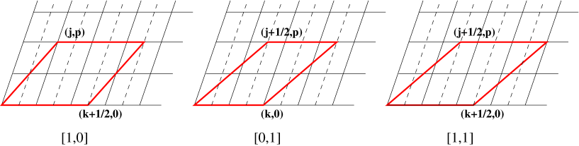
Figure 3: The three possible types of $E1_{r}$ multi-instantons, $[h,g]=\{[1,0],[0,1],[1,1]\}$, wrapping torsional cycles in the $r$-th 2-torus in the $SO(q)\times SO(32-q)$ model, with induced worldvolume complex structure $\mathcal{U}_{r}^{[h,g]}$ given in eq.(58). The continues lines represent the lattice of the underlying 2-torus. The orbifold generator reversing the transverse coordinates to the instanton, shifts the lattice to the dashed one.

Subtracting the gauge group dependent part, along the lines of eqs.(7) and (8), we obtain the following corrections to the effective Kähler potential and gauge kinetic function,

$$K=-\textrm{log}(S+\bar{S})-\sum_{i=1}^{3}\textrm{log}[(T_{i}+\bar{T}_{i})(U_{i}+\bar{U}_{i})]+\frac{1}{2}\sum_{i=1}^{3}\frac{V^{i}_{1-loop}+V^{i}_{E1}}{S+\bar{S}}\ ,$$ (59)

$$V^{1}_{1-loop}=\frac{62\pi}{45}\frac{E_{1/2}(iU_{1},2)}{T_{1}+\bar{T}_{1}}\ ,$$ (60)

$$V^{r}_{1-loop}=\frac{\pi}{180}(q^{2}-32q+248)\frac{E_{1/2}(iU_{r},2)}{T_{r}+\bar{T}_{r}}\ ,$$ (61)

$$V^{1}_{E1}=-\sum_{k>j\geq 0,\ p>0}\sum_{[h,g]}\frac{(-1)^{gk+hj}}{p^{2}k_{h}^{2}}e^{-2\pi pk_{h}T_{1}}$$ (62)

$$\quad\times\left[\frac{\hat{\mathcal{A}}_{K,1}^{[h,g]}\left(\mathcal{U}_{1}^{[h,g]}\right)}{T_{1}+\bar{T}_{1}}-\frac{i\pi pk_{h}}{\mathcal{U}_{1}^{[h,g]}-\bar{\mathcal{U}}_{1}^{[h,g]}}\chi_{1}\left[{h\atop g}\right](\mathcal{U}_{1}^{[h,g]})\right]\ +\ \textrm{c.c.}$$

$$V^{r}_{E1}=-\sum_{k>j\geq 0,\ p>0}\sum_{[h,g]}\frac{(-1)^{(hj+gk)\left(\frac{q}{4}+1\right)}}{p^{2}k_{h}^{2}}e^{-2\pi pk_{h}T_{r}}$$ (63)

$$\quad\times\left[\frac{\hat{\mathcal{A}}_{K,2}^{[h,g]}\left(\mathcal{U}_{r}^{[h,g]}\right)}{T_{r}+\bar{T}_{r}}-\frac{i\pi pk_{h}}{\mathcal{U}_{r}^{[h,g]}-\bar{\mathcal{U}}_{r}^{[h,g]}}\chi_{2}\left[{h\atop g}\right](\mathcal{U}_{r}^{[h,g]})\right]\ +\ \textrm{c.c.}\ ,$$

$$f_{SO(q)}=S+\frac{15\pi}{2}U_{1}+30\textrm{log }\vartheta_{2}(iU_{1})+(q-17)\sum_{r=2,3}\left[\frac{\pi}{2}U_{r}+2\textrm{log }\vartheta_{2}(iU_{r})\right]-$$ (64)

$$\qquad\qquad-\frac{1}{2}\sum_{k>j\geq 0,\ p>0}\sum_{[h,g]}\frac{(-1)^{gk+hj}}{pk_{h}}\left[e^{-2\pi pk_{h}T_{1}}\mathcal{A}_{f,1}^{[h,g]}(\mathcal{U}_{1}^{[h,g]})+\right.$$

$$\left.\qquad\qquad\qquad\qquad\qquad\qquad+\sum_{r=2,3}(-1)^{(hj+gk)\frac{q}{4}}e^{-2\pi pk_{h}T_{r}}\mathcal{A}_{f,2}^{[h,g]}(\mathcal{U}_{r}^{[h,g]})\right]\ ,$$

where $\mathcal{A}_{f,i}^{[h,g]}$ is defined as $\hat{\mathcal{A}}_{f,i}^{[h,g]}$, but replacing $\hat{E}_{2}$ by $E_{2}$, and we have introduced the notation,

$$\chi_{1}\left[{h\atop g}\right](\tau)\equiv\frac{4(\chi_{o}+\chi_{v})}{\eta^{2}\vartheta\left[{1-h\atop 1-g}\right]^{2}}\ , \chi_{2}\left[{0\atop 1}\right](\tau)\equiv\frac{\chi_{o}-\chi_{v}}{\eta^{8}}\vartheta_{3}^{2}\vartheta_{4}^{2}\ ,$$

$$\chi_{2}\left[{1\atop 0}\right](\tau)\equiv\chi_{2}\left[{0\atop 1}\right](S\tau)\ , \chi_{2}\left[{1\atop 1}\right](\tau)\equiv\chi_{2}\left[{0\atop 1}\right](ST^{-1}\tau)\ .$$

Several comments are in order. First, notice that the field theory result for the $\beta$-function coefficient, (39), is correctly reproduced. The overall structure of the non-perturbative and loop corrections is very similar to the ones in the BSGP orbifold, but the standard Eisenstein series and Hecke operators are replaced by the corresponding automorphic forms of $\Gamma_{0}(2)$. Moreover, there is a non-trivial dependence of the non-perturbative dynamics on the rank of the gauge group, through the phases $\textrm{exp}[i\pi(hj+gk)\frac{q}{4}]$. These would explain why in the heterotic side the orbifold action on the winding modes is very different, depending on the value of $q$ (c.f. eq.(41)). This behavior may resemble in spirit the more familiar situation of ordinary gauge theory instantons, where their contributions are often subjected to constraints depending on the ranks of the gauge group.

By a direct inspection of (55), it is easy to check the fact that instantonic corrections are gauge-group independent when they come from instantons which are left invariant by the orbifold operations acting trivially on the gauge degrees of freedom; whereas they are gauge-group dependent if they come from instantons left invariant by the orbifold operations which act non-trivially on the gauge degrees of freedom.

Finally, let us mention the possibility of additional non-perturbative corrections coming from purely $\mathcal{N}=1$ sectors, not considered here. Precisely, in [24] it was argued for the $q=32$ case, the presence of extra non-perturbative contributions to the gauge thresholds, due to the combined effect of multi-instantons wrapping different cycles of the internal space.

4 Universality of $\mathcal{N}=2$ corrections

It has been pointed out very often in the literature the importance of global symmetries in determining the expression of non-perturbative and $\alpha^{\prime}$ corrections which come from BPS states [28]. The results in the previous sections, based on the S-duality map, reveal that the string loop and $E1$ multi-instanton effects coming from $\mathcal{N}=2$ subsectors of the theory arise in terms of non-holomorphic Eisenstein series and Hecke operators relevant to the global symmetry preserved by the orbifold. In this section, we elaborate on certain “universality” of the $\mathcal{N}=2$ corrections computed in the BSGP orbifold. Similar aspects have been discussed in the context of $\alpha^{\prime}$ corrections to the gauge couplings in heterotic compactifications [34, 36, 20, 37].

Precisely, we would like to consider toroidal orbifold compactifications on which the orbifold action, $\mathbb{G}$, contains some subgroup, $\mathbb{G}^{i}$, leaving unrotated a given complex plane. The contribution of these sectors to the threshold corrections to the physical gauge couplings can be expressed as,

$$\Lambda_{a}=-\frac{1}{8}\sum_{i}\int_{\mathcal{F}}\frac{d^{2}\tau}{\tau_{2}}\hat{Z}_{i}\hat{\mathcal{A}}^{a}_{f,i}\ ,$$ (65)

where the sum runs over the disjoint union of $\mathcal{N}=2$ subsectors, each leaving invariant a single complex plane, and the gauge group is given by a product $G=\prod_{a}G_{a}$. The lattice sums, $\hat{Z}_{i}$, are given in eq.(11), where $T_{i}$ and $U_{i}$ are now the Kähler and complex structure moduli of the corresponding unrotated complex plane. Moreover, $\hat{\mathcal{A}}^{a}_{f,i}\sim M^{a}_{i}/\eta^{24}$, with $M^{a}_{i}$ an almost holomorphic modular form of degree 24.

The space of holomorphic forms of degree 24 is a vector space of dimension 2, engendered by the Eisenstein series $E_{6}^{2}$ and $E_{4}^{3}$ [43, 44]. If we also allow for almost holomorphic modular forms, we have to include in addition $\hat{E}_{2}E_{10}$. Hence $M_{i}^{a}$ is in general determined by three coefficients, which usually can be obtained from the low energy spectrum. More precisely, imposing the absence of tachyons in the spectrum, we obtain,

$$\hat{\mathcal{A}}^{a}_{f,i}=2b_{i}^{a}+\frac{\gamma_{i}}{20\eta^{24}}\left[D_{10}E_{10}-528\eta^{24}\right]\ ,$$ (66)

where $b_{i}^{a}$ is the $\beta$-function coefficient of the $\mathcal{N}=2$ gauge theory associated to a would-be $T^{6}/\mathbb{G}^{i}$ orbifold, $\gamma_{i}$ is a model dependent (but gauge group independent) coefficient to be determined, and we have made use of the identities,

$$D_{10}E_{10}=\frac{2}{3}E_{6}^{2}+E_{4}^{3}-\frac{5}{3}\hat{E}_{2}E_{10}\ ,\qquad\eta^{24}=\frac{1}{2^{6}\cdot 3^{3}}[E_{4}^{3}-E_{6}^{2}]\ .$$ (67)

Proceeding as in section 2.2 we get,

$$\Lambda_{a}=\sum_{i}\bigg{\{}\frac{\pi(b_{i}^{a}+6\gamma_{i})}{12}\textrm{Re }T_{i}\ +\ \frac{\pi\gamma_{i}}{3}\frac{E(iU_{i},2)}{T_{i}+\bar{T}_{i}}\ -\\ -\frac{1}{4}\left(\sum_{k>j\geq 0,p>0}\frac{1}{kp}e^{-2\pi pkT_{i}}\left[\hat{\mathcal{A}}^{a}_{f,i}(\mathcal{U}_{i})-\frac{\gamma_{i}}{\pi kp}\frac{\hat{\mathcal{A}}_{K}(\mathcal{U}_{i})}{T_{i}+\bar{T}_{i}}\right]\ +\ \textrm{c.c.}\right)\ -\\ -\ \frac{b_{i}^{a}}{4}\left(\textrm{log}|\eta(iU_{i})|^{4}+\textrm{log}[(\textrm{Re }U_{i})(\textrm{Re }T_{i})\mu^{2}]\right)\bigg{\}}\ ,$$ (68)

with $\hat{\mathcal{A}}_{K}$ and $\mathcal{U}_{i}$ defined in (25) and (26), respectively. From this expression, we can then extract the corrected Kähler potential and gauge kinetic functions of the effective theory, as we did in previous sections, obtaining

$$K=-\textrm{log}(S+\bar{S})-\sum_{i}\bigg{\{}\textrm{log}[(T_{i}+\bar{T}_{i})(U_{i}+\bar{U}_{i})]+\frac{1}{2}\frac{V^{i}_{1-loop}+V^{i}_{E1}}{S+\bar{S}}\bigg{\}}+\ldots\ ,$$ (69)

$$V^{i}_{1-loop}=\frac{4\pi\gamma_{i}}{3}\frac{E(iU_{i},2)}{T_{i}+\bar{T}_{i}}\ ,$$ (70)

$$V^{i}_{E1}=\frac{\gamma_{i}}{\pi}\sum_{k>j\geq 0,\ p>0}\frac{e^{-2\pi kpT_{i}}}{(kp)^{2}}\left[\frac{\hat{\mathcal{A}}_{K}(\mathcal{U}_{i})}{T_{i}+\bar{T}_{i}}-\frac{2ikp}{\mathcal{U}_{i}-\bar{\mathcal{U}_{i}}}\frac{E_{10}(\mathcal{U}_{i})}{\eta^{24}(\mathcal{U}_{i})}\right]\ +\ \textrm{c.c.}\ ,$$ (71)

$$f_{a}=S+\sum_{i}\bigg{\{}\frac{\pi(b_{i}^{a}+6\gamma_{i})T_{i}}{12}-b^{a}_{i}\textrm{log }\eta(iU_{i})-\frac{1}{2}\sum_{k>j\geq 0,\ p>0}\frac{e^{-2\pi kpT_{i}}}{kp}\mathcal{A}^{a}_{f,i}(\mathcal{U}_{i})\bigg{\}}+\ldots\ ,$$ (72)

where the dots refer to possible additional corrections from other sectors. The interpretation of these terms is similar to the one discussed in sections 2.2 and 2.3.

Notice that these expressions in principle also apply in orbifolds where the heterotic S-dual description is unknown, and therefore our technique in principle no longer applies. It would be very interesting to obtain the general formula for the $\mathcal{N}=2$ corrections by direct computation in the type I orbifold, and to see whether there is agreement with our conjectured expression.

5 Concluding remarks

In the present paper we explicitly computed the $E1$ instantonic corrections to the gauge kinetic function $f$ and to the Kähler potential $K$ in ${\cal N}=2$ and ${\cal N}=1$ type I string vacua which have known heterotic S-duals. We showed that one-loop threshold corrections to gauge couplings in the heterotic dual encode one-loop and instantonic corrections for both $f$ and $K$ on the type I side, whereas the corresponding direct one-loop type I threshold correction misses the one-loop correction to the Kähler potential, computed by other methods in [1] and [2]. We gave arguments based on target-space modular invariance on universality properties of instantonic corrections in ${\cal N}=2$ vacua. It is clear however that our results apply to the much larger class of models of ${\cal N}=1$ type I models with ${\cal N}=2$ subsectors, like for example the $\mathbb{Z}_{6}$, $\mathbb{Z}_{6}^{\prime}$, $\mathbb{Z}_{8}$ or $\mathbb{Z}_{12}$ type I orbifolds.

We performed a similar computation in dual pairs in compactifications on smooth Calabi-Yau spaces which have an exact CFT description, based on a recently worked out class of freely-acting S-dual pairs [16]. We showed that even if the heterotic duals of perturbatively connected type I models have different orbifold actions in the twisted (winding) sector, the S-duality maps correctly heterotic $\alpha^{\prime}$ corrections into type I instantonic corrections. As a byproduct, we also checked the intuitively obvious statement that instantonic corrections are gauge-group independent if coming from instantons left invariant by orbifold operations acting trivially on the gauge degrees of freedom, whereas they are gauge-group dependent if coming from instantons left invariant by orbifold operations acting non-trivially on the gauge degrees of freedom.

As already argued in [16], it is clear that whereas our discussion was focused on multi-instantonic corrections to the gauge kinetic function and the Kähler potential, similar multi-instanton corrections are expected to occur for the superpotential. A simple argument can be given in the case (explicitly realized by the string construction of [16]) where non-perturbative gauge (E5 instantonic) effects occur on D9-branes, leading to a superpotential,

$$W_{np}\ =e^{-b(S+f_{1}(U_{i})+f_{np}(U_{i},T_{i}))}\ =\ \sum_{n}c_{n}(U_{i})\ e^{-2\pi nT}\ e^{-bS}\$$ (73)

Whereas non-perturbative corrections to the superpotential are well-known to play a crucial role in moduli stabilization [10], we expect that instantonic corrections to the Kähler potential may play also an important role in some scenarios of moduli stabilization, for example in the large-volume scenario [13]. Moreover, the instantonic corrections to the gauge kinetic function are expected to modify the gauge couplings and gaugino masses, and in particular may become relevant in concrete phenomenological models.

Another interesting direction which our paper has left partially open is the detailed type I microscopic derivation of the multi-instanton effects obtained here from S-duality, which should involve in an important way the lifting of fermionic zero-modes by instanton interactions along the lines of [48, 49].

It would be, finally, very instructive to perform similar studies in the S-dual pairs of $\mathcal{N}=1$ orbifold models conjectured in [50, 51] and learn more about non-perturbative dynamics of both sides using $\alpha^{\prime}$ corrections on the heterotic side and instantonic computations on the type I side.

Appendix A Details on the computations

A.1 The BSGP model

A.1.1 Elliptic genera

In order to express the elliptic genus in terms of ordinary modular forms we use the following relations,

$$\vartheta^{4}\left[{0\atop\pm 1/2}\right] =\frac{1}{2}\vartheta_{3}\vartheta_{4}(\vartheta_{3}^{2}+\vartheta_{4}^{2})\ , \vartheta^{4}\left[{1\atop\pm 1/2}\right] =\frac{\vartheta_{2}^{3}\eta^{3}}{\vartheta_{3}^{2}+\vartheta_{4}^{2}}\ ,$$ (74)

$$\vartheta^{4}\left[{\pm 1/2\atop 0}\right] =\frac{1}{2}\vartheta_{2}\vartheta_{3}(\vartheta_{2}^{2}+\vartheta_{3}^{2})\ , \vartheta^{4}\left[{\pm 1/2\atop 1}\right] =-\frac{\vartheta_{4}^{3}\eta^{3}}{\vartheta_{2}^{2}+\vartheta_{3}^{2}}\ ,$$ (75)

$$\vartheta^{4}\left[{\pm 1/2\atop\pm 1/2}\right] =\frac{1}{2}\vartheta_{2}\vartheta_{4}(\vartheta_{2}^{2}-i\vartheta_{4}^{2})\ , \vartheta^{4}\left[{\pm 1/2\atop\mp 1/2}\right] =\frac{\vartheta_{3}^{3}\eta^{3}}{\vartheta_{2}^{2}-i\vartheta_{4}^{2}}\ ,$$ (76)

and,

$$\frac{\vartheta^{\prime\prime}\left[{0\atop\pm 1/2}\right]}{\vartheta\left[{0\atop\pm 1/2}\right]} =\frac{i\pi^{3}}{3}(4E_{2}+\vartheta_{3}^{4}-6\vartheta_{3}^{2}\vartheta_{4}^{2}+\vartheta_{4}^{4})\ ,$$ (77)

$$\frac{\vartheta^{\prime\prime}\left[{1\atop\pm 1/2}\right]}{\vartheta\left[{1\atop\pm 1/2}\right]} =\frac{i\pi^{3}}{3}(4E_{2}+\vartheta_{3}^{4}+6\vartheta_{3}^{2}\vartheta_{4}^{2}+\vartheta_{4}^{4})\ ,$$ (78)

$$\frac{\vartheta^{\prime\prime}\left[{\pm 1/2\atop 0}\right]}{\vartheta\left[{\pm 1/2\atop 0}\right]} =\frac{i\pi^{3}}{3}\left(4E_{2}+4\vartheta_{3}^{4}+\frac{(\vartheta_{2}^{2}-5\vartheta_{3}^{2})\vartheta_{4}^{4}}{\vartheta_{2}^{2}+\vartheta_{3}^{2}}\right)\ ,$$ (79)

$$\frac{\vartheta^{\prime\prime}\left[{\pm 1/2\atop 1}\right]}{\vartheta\left[{\pm 1/2\atop 1}\right]} =\frac{i\pi^{3}}{3}\left(4E_{2}-8\vartheta_{3}^{4}+\frac{(\vartheta_{2}^{2}+7\vartheta_{3}^{2})\vartheta_{4}^{4}}{\vartheta_{2}^{2}+\vartheta_{3}^{2}}\right)\ ,$$ (80)

$$\frac{\vartheta^{\prime\prime}\left[{\pm 1/2\atop\pm 1/2}\right]}{\vartheta\left[{\pm 1/2\atop\pm 1/2}\right]} =\frac{i\pi^{3}}{3}\left(4E_{2}-8\vartheta_{4}^{4}+7\vartheta_{3}^{4}-\frac{6\vartheta_{2}^{2}\vartheta_{3}^{4}}{\vartheta_{2}^{2}-i\vartheta_{4}^{2}}\right)\ ,$$ (81)

$$\frac{\vartheta^{\prime\prime}\left[{\pm 1/2\atop\mp 1/2}\right]}{\vartheta\left[{\pm 1/2\atop\mp 1/2}\right]} =\frac{i\pi^{3}}{3}\left(4E_{2}+4\vartheta_{4}^{4}-5\vartheta_{3}^{4}+\frac{6\vartheta_{2}^{2}\vartheta_{3}^{4}}{\vartheta_{2}^{2}-i\vartheta_{4}^{2}}\right)\ .$$ (82)

Then it is possible to show that,

$$A_{1} \equiv 2\left(\bar{\Gamma}\left[{0\atop 1}\right]\vartheta_{3}^{2}\vartheta_{4}^{2}+\bar{\Gamma}\left[{1\atop 0}\right]\vartheta_{2}^{2}\vartheta_{3}^{2}+\bar{\Gamma}\left[{1\atop 1}\right]\vartheta_{2}^{2}\vartheta_{4}^{2}\right)=\frac{2E_{4}E_{6}}{\eta^{16}}=\frac{2E_{10}}{\eta^{16}}\ ,$$ (83)

$$A_{2} \equiv\partial^{2}_{\nu_{1}}A_{1}=-\frac{2\pi^{2}}{3\eta^{16}}(E_{2}E_{4}E_{6}-\frac{5}{12}E_{6}^{2}-\frac{7}{12}E_{4}^{3}),$$ (84)

where $\partial_{\nu_{1}}$ acts on the first $SO(2)$ character in $\bar{\Gamma}\left[{h\atop g}\right]$, with affine parameter $\nu_{1}$. Therefore,

$$\hat{\mathcal{A}}_{f}\equiv-\frac{1}{8\pi\bar{\eta}^{8}}\left(\frac{A_{1}}{\tau_{2}}+\frac{A_{2}}{\pi}\right)=\frac{1}{12\eta^{24}}(\hat{E}_{2}E_{10}-\frac{5}{12}E_{6}^{2}-\frac{7}{12}E_{4}^{3})=-24+\frac{60}{\pi\tau_{2}}+\ldots$$ (85)

The other modular form that we will need in the computation of the thresholds is,

$$\hat{\mathcal{A}}_{K}\equiv\frac{1}{4\pi}\left(i\partial_{\tau}-\frac{1}{\tau_{2}}\right)\frac{E_{10}}{\eta^{24}}$$ (86)

Taking into account that $E_{10}=E_{4}E_{6}$ and,

$$\partial_{\tau}E_{4}=-\frac{2\pi i}{3}(E_{6}-E_{2}E_{4})\ ,\qquad\partial_{\tau}E_{6}=-\pi i(E_{4}^{2}-E_{2}E_{6})\ ,$$ (87)

we then obtain,

$$\hat{\mathcal{A}}_{K}=\frac{1}{12\eta^{24}}(\hat{E}_{2}E_{4}E_{6}+2E_{6}^{2}+3E_{4}^{3})\ .$$ (88)

A.1.2 Zero orbit

For the zero orbit we have the contribution,

$$\Lambda_{0}=-\frac{\textrm{Re }T_{1}}{8}\int_{\mathcal{F}}\frac{d^{2}\tau}{\tau_{2}^{2}}\hat{\mathcal{A}}_{f}=\\ =-\frac{\textrm{Re }T_{1}}{96}\int_{\mathcal{F}}\frac{d^{2}\tau}{\tau_{2}^{2}}\left[\hat{E}_{2}(e^{-2\pi i\tau}-240+\ldots)-e^{-2\pi i\tau}-24+\ldots\right]$$ (89)

Making use of the formula [45],

$$\int_{\mathcal{F}}\frac{d^{2}\tau}{\tau_{2}^{2}}(\hat{E}_{2})^{r}(c_{-1}e^{-2\pi i\tau}+c_{0}+\ldots)=\frac{\pi}{3(r+1)}[c_{0}-24(r+1)c_{-1}]\ ,$$ (90)

we get,

$$\Lambda_{0}=\frac{\pi}{2}(\textrm{Re }T_{1})\ .$$ (91)

A.1.3 Degenerate orbits

In this case we have to compute the contribution,

$$\Lambda_{d}=-\frac{\textrm{Re }T_{1}}{8}\int_{\mathcal{F}_{T}}\frac{d^{2}\tau}{\tau_{2}^{2}}\left(\frac{60}{\pi\tau_{2}}-24+\mathcal{O}(e^{2\pi i\tau})\right)\sum_{j,p}\textrm{exp}\left[-\frac{\pi\textrm{Re }T_{1}}{\tau_{2}\textrm{Re }U_{1}}|j+ipU_{1}|^{2}\right]$$ (92)

where the integration region, $\mathcal{F}_{T}$, corresponds to the upper band $\{|\tau_{1}|<1/2,\ \tau_{2}>0\}$. This can be done using the formula [29],

$$\int_{\mathcal{F}_{T}}\frac{d^{2}\tau}{\tau_{2}^{1+r}}\sum_{j,p}\textrm{exp}\left[-\frac{\pi\textrm{Re }T}{\tau_{2}\textrm{Re }U}|j+ipU|^{2}\right]=\frac{2\Gamma(r)\zeta(2r)}{(\pi\textrm{Re }T)^{r}}E(iU,r)\ .$$ (93)

Taking into account that,

$$E(iU,1)=-\frac{3}{\pi}(\textrm{log }|\eta(iU)|^{4}+\textrm{log }[(\textrm{Re }T)(\textrm{Re }U)]\mu^{2})\ +\ \textrm{const.}\ ,$$ (94)

with $\mu^{2}$ the infrared regulator and “const.” a renormalization scheme dependent constant which we will disregard in what follows, we obtain,

$$\Lambda_{d}=-3(\textrm{log }|\eta(iU_{1})|^{4}+\textrm{log }[(\textrm{Re }T_{1})(\textrm{Re }U_{1})\mu^{2}])-\frac{\pi}{3}\frac{E(iU_{1},2)}{T_{1}+\bar{T}_{1}}\ .$$ (95)

A.1.4 Non-degenerate orbits

Finally, for non-degenerate orbits we need to compute,

$$\Lambda_{nd}=-\frac{\textrm{Re }T_{1}}{4}\int_{\mathbb{C}^{+}}\frac{d^{2}\tau}{\tau_{2}^{2}}\sum_{k>j\geq 0,\ p\neq 0}\sum_{n}\left(d_{1}(n)-\frac{d_{2}(n)}{4\pi\tau_{2}}\right)\ \times\\ \times\ e^{2\pi i\tau n}\textrm{exp}\left[-2\pi T_{1}kp-\frac{\pi\textrm{Re }T_{1}}{\tau_{2}\textrm{Re }U_{1}}|-j-iU_{1}p+k\tau|^{2}\right]\ ,$$ (96)

where we have expanded,

$$\mathcal{A}_{f}=\sum_{n}d_{1}(n)e^{2\pi in\tau}\ ,\qquad\frac{E_{10}}{\eta^{24}}=\sum_{n}d_{2}(n)e^{2\pi in\tau}$$ (97)

Performing first the integration on $\tau_{1}$,

$$\Lambda_{nd}=-\frac{[(\textrm{Re }T_{1})(\textrm{Re }U_{1})]^{1/2}}{4}\sum_{k>j\geq 0,\ p\neq 0}\sum_{n}\int_{0}^{\infty}\frac{d\tau_{2}}{\tau_{2}^{3/2}}\frac{1}{k}\left(d_{1}(n)-\frac{d_{2}(n)}{4\pi\tau_{2}}\right)\times\\ \times\ \textrm{exp}\left[-2\pi i(\textrm{Im }T_{1})kp+2\pi in\left(\frac{j-p(\textrm{Im }U_{1})}{k}\right)\right]\\ \times\ \textrm{exp}\left[-\frac{\pi(\textrm{Re }T_{1})}{\textrm{Re }U_{1}}\left(k+\frac{n(\textrm{Re }U_{1})}{k(\textrm{Re }T_{1})}\right)^{2}\tau_{2}-\frac{\pi p^{2}(\textrm{Re }T_{1})(\textrm{Re }U_{1})}{\tau_{2}}\right]$$

Then the integral on $\tau_{2}$ can be carried out with the aid of,

$$\int_{0}^{\infty}\frac{dx}{x^{3/2}}e^{-ax-b/x}=\sqrt{\frac{\pi}{b}}e^{-2\sqrt{ab}}\ ,$$ (98)

$$\int_{0}^{\infty}\frac{dx}{x^{5/2}}e^{-ax-b/x}=\left(\frac{1}{2b}+\sqrt{\frac{a}{b}}\right)\sqrt{\frac{\pi}{b}}e^{-2\sqrt{ab}}\ .$$ (99)

And summing over $n$, we finally get,

$$\Lambda_{nd}=-\frac{1}{4}\sum_{k>j\geq 0,\ p>0}\frac{e^{-2\pi kpT_{1}}}{kp}\left(\hat{\mathcal{A}}_{f}(\mathcal{U})+\frac{1}{\pi kp(T_{1}+\bar{T}_{1})}\hat{\mathcal{A}}_{K}(\mathcal{U})\right)\ +\ \textrm{c.c.}$$ (100)

with $\hat{\mathcal{A}}_{f}$, $\hat{\mathcal{A}}_{K}$ and $\mathcal{U}$ defined in (21), (25) and (26), respectively.

A.2 The $SO(q)\times SO(32-q)$ model

A.2.1 Elliptic genera

The relevant characters for this model are,

$$\chi_{o}+\chi_{v}=\frac{E_{4}^{2}}{\eta^{16}}\ ,\qquad\chi_{o}-\chi_{v}=\frac{1}{2\eta^{16}}(\vartheta_{3}^{q/2}\vartheta_{4}^{16-q/2}+\vartheta_{4}^{q/2}\vartheta_{3}^{16-q/2})$$ (101)

Then, it is possible to show that,

$$\hat{\mathcal{A}}_{f,1}^{[0,1]}\equiv -\frac{\vartheta_{3}^{2}\vartheta_{4}^{2}}{4\pi\eta^{8}}\left(\frac{1}{\tau_{2}}+\frac{\partial^{2}_{\nu_{1}}}{\pi}\right)(\chi_{o}+\chi_{v})=\frac{\vartheta_{3}^{2}\vartheta_{4}^{2}E_{4}(\hat{E}_{2}E_{4}-E_{6})}{12\eta^{24}}=60-\frac{124}{\pi\tau_{2}}+\ldots$$ (102)

$$\hat{\mathcal{A}}_{f,2}^{[0,1]}\equiv -\frac{\vartheta_{3}^{2}\vartheta_{4}^{2}}{4\pi\eta^{8}}\left(\frac{1}{\tau_{2}}+\frac{\partial^{2}_{\nu_{1}}}{\pi}\right)(\chi_{o}-\chi_{v})=$$

$$\qquad\frac{\vartheta_{3}^{2}\vartheta_{4}^{2}}{24\eta^{24}}\left[\vartheta_{3}^{q/2}\vartheta_{4}^{16-q/2}(\hat{E}_{2}+\vartheta_{2}^{4}-\vartheta_{4}^{4})+\vartheta_{4}^{q/2}\vartheta_{3}^{16-q/2}(\hat{E}_{2}-\vartheta_{2}^{4}-\vartheta_{3}^{4})\right]=$$ (103)

$$\qquad\qquad\qquad\qquad=4(q-17)-\frac{q^{2}-32q-248}{2\pi\tau_{2}}+\ldots\ .$$

The other modular forms that we need are,

$$\hat{\mathcal{A}}_{K,1}^{[0,1]}\equiv\frac{1}{4\pi}\left(i\partial_{\tau}-\frac{1}{\tau_{2}}\right)\frac{(E_{4}\vartheta_{3}\vartheta_{4})^{2}}{\eta^{24}}=\frac{E_{4}\vartheta_{3}^{2}\vartheta_{4}^{2}}{24\eta^{24}}[8E_{6}+E_{4}(\vartheta_{4}^{4}+\vartheta_{3}^{4})+2\hat{E}_{2}E_{4}]$$ (104)

$$\hat{\mathcal{A}}_{K,2}^{[0,1]}\equiv\frac{1}{4\pi}\left(i\partial_{\tau}-\frac{1}{\tau_{2}}\right)\frac{\vartheta_{3}^{2}\vartheta_{4}^{2}}{2\eta^{24}}(\vartheta_{3}^{q/2}\vartheta_{4}^{16-q/2}+\vartheta_{4}^{q/2}\vartheta_{3}^{16-q/2})=$$

$$\qquad=\frac{\vartheta_{3}^{2}\vartheta_{4}^{2}}{96\eta^{24}}\left[\vartheta_{4}^{16-q/2}\vartheta_{3}^{q/2}\left(8\hat{E}_{2}+\left(14-\frac{3q}{2}\right)\vartheta_{2}^{4}+20\vartheta_{3}^{4}\right)+\right.$$

$$\qquad\qquad\qquad\qquad\qquad\left.+\vartheta_{3}^{16-q/2}\vartheta_{4}^{q/2}\left(8\hat{E}_{2}-\left(14-\frac{3q}{2}\right)\vartheta_{2}^{4}+20\vartheta_{4}^{4}\right)\right]\ ,$$ (105)

Finally, we define $S$ and the $ST^{-1}$ transformed forms,

$$\hat{\mathcal{A}}_{f,i}^{[1,0]}(\tau) =\hat{\mathcal{A}}_{f,i}^{[0,1]}(S\tau)\ , \hat{\mathcal{A}}_{f,i}^{[1,1]}(\tau) =\hat{\mathcal{A}}_{f,i}^{[0,1]}(ST^{-1}\tau)\ ,$$ (106)

$$\hat{\mathcal{A}}_{K,i}^{[1,0]}(\tau) =\hat{\mathcal{A}}_{K,i}^{[0,1]}(S\tau)\ , \hat{\mathcal{A}}_{K,i}^{[1,1]}(\tau) =\hat{\mathcal{A}}_{K,i}^{[0,1]}(ST^{-1}\tau)\ .$$ (107)

for $i=1,2$.

A.2.2 Degenerate orbits

For the degenerate orbits we have the contribution,

$$\Lambda_{d}=-\frac{1}{8}\int_{\mathcal{F}_{T}}\frac{d^{2}\tau}{\tau_{2}^{2}}\sum_{p,j}\{\left(60-\frac{124}{\pi\tau_{2}}+\ldots\right)(\textrm{Re }T_{1})\textrm{exp}\left[-\frac{\pi\textrm{Re }T_{1}}{\tau_{2}\textrm{Re }U_{1}}\left|j+\frac{1}{2}+ipU_{1}\right|^{2}\right]+\\ \sum_{r=2,3}\left(4(q-17)-\frac{q^{2}-32q-248}{2\pi\tau_{2}}+\ldots\right)(\textrm{Re }T_{r})\textrm{exp}\left[-\frac{\pi\textrm{Re }T_{r}}{\tau_{2}\textrm{Re }U_{r}}\left|j+\frac{1}{2}+ipU_{r}\right|^{2}\right]\}\ ,$$

where the dots correspond to order $\mathcal{O}(e^{2\pi i\tau})$ terms not contributing to the final expression. Proceeding as in section A.1.3, we obtain,

$$\Lambda_{d}=-\frac{\pi}{2}\left[5E_{1/2}(iU_{1},1)+\frac{q-17}{3}\sum_{r=2,3}E_{1/2}(iU_{r},1)\right]+\\ +\frac{\pi}{360}\left[124\frac{E_{1/2}(iU_{1},2)}{T_{1}+\bar{T}_{1}}+\frac{1}{2}\sum_{r=2,3}(q^{2}-32q+248)\frac{E_{1/2}(iU_{r},2)}{T_{r}+\bar{T}_{r}}\right]\ ,$$ (108)

with $E_{1/2}(U,k)$ the shifted non-holomorphic Eisenstein series defined in (56).

A.2.3 Non-degenerate orbits

We begin computing the contribution from non-degenerate orbits of type I. This is given by,

$$\Lambda_{nd_{I}}=-\frac{1}{4}\int_{\mathbb{C}^{+}}\frac{d^{2}\tau}{\tau_{2}^{2}}\sum_{p\neq 0,k>j\geq 0}\sum_{n=0}^{\infty}e^{2\pi i\tau n}(-1)^{k}\\ \left[(\textrm{Re }T_{1})\left(d_{1}(n)-\frac{d_{2}(n)}{4\pi\tau_{2}}\right)\textrm{exp}\left(-2\pi kpT_{1}-\frac{\pi\textrm{Re }T_{1}}{\tau_{2}\textrm{Re }U_{1}}|k\tau-j-\frac{1}{2}-ipU_{1}|^{2}\right)+\right.\\ \left.\sum_{i=2,3}(\textrm{Re }T_{i})\left(d_{3}(n)-\frac{d_{4}(n)}{4\pi\tau_{2}}\right)(-1)^{\frac{qk}{4}}\textrm{exp}\left(-2\pi kpT_{i}-\frac{\pi\textrm{Re }T_{i}}{\tau_{2}\textrm{Re }U_{i}}|k\tau-j-\frac{1}{2}-ipU_{i}|^{2}\right)\right]$$

where we have performed the expansions,

$$\mathcal{A}_{f,1}^{[0,1]} =\sum_{n}d_{1}(n)e^{2\pi i\tau n}\ , \frac{(E_{4}\vartheta_{3}\vartheta_{4})^{2}}{\eta^{24}} =\sum_{n}d_{2}(n)e^{2\pi i\tau n}\ ,$$

$$\mathcal{A}_{f,2}^{[0,1]} =\sum_{n}d_{3}(n)e^{2\pi i\tau n}\ , \frac{(\vartheta_{3}\vartheta_{4})^{2}}{2\eta^{24}}(\vartheta_{3}^{q/2}\vartheta_{4}^{16-q/2}+\vartheta_{4}^{q/2}\vartheta_{3}^{16-q/2}) =\sum_{n}d_{4}(n)e^{2\pi i\tau n}\ .$$

Proceeding exactly in the same way as in section A.1.4, we obtain,

$$\Lambda_{nd_{I}}=-\frac{1}{4}\sum_{p>0,k>j\geq 0}\frac{(-1)^{k}}{pk}\left[e^{-2\pi pkT_{1}}\left(\hat{\mathcal{A}}_{f,1}^{[0,1]}(\mathcal{U}_{1}^{[0,1]})+\frac{\hat{\mathcal{A}}_{K,1}^{[0,1]}(\mathcal{U}_{1}^{[0,1]})}{\pi kp(T_{1}+\bar{T}_{1})}\right)\right.\\ \left.+\sum_{r=2,3}(-1)^{\frac{kq}{4}}e^{-2\pi rkT_{r}}\left(\hat{\mathcal{A}}_{f,2}^{[0,1]}(\mathcal{U}_{r}^{[0,1]})+\frac{\hat{\mathcal{A}}_{K,2}^{[0,1]}(\mathcal{U}_{r}^{[0,1]})}{\pi kp(T_{r}+\bar{T}_{r})}\right)\right]\ +\ \textrm{c.c.}\ ,$$ (109)

with $\mathcal{U}_{r}^{[h,g]}$ defined in (58).

For type II (type III) non-degenerate orbits we proceed in the same way, but performing a change of variables by the corresponding coset representative, $\tau\to S\tau$ ($\tau\to ST^{-1}\tau$), obtaining,

$$\Lambda_{nd_{II}}=-\frac{1}{4}\sum_{p>0,k>j\geq 0}\frac{(-1)^{j}}{p\left(k+\frac{1}{2}\right)}\left[e^{-2\pi p\left(k+\frac{1}{2}\right)T_{1}}\left(\hat{\mathcal{A}}_{f,1}^{[1,0]}(\mathcal{U}_{1}^{[1,0]})+\frac{\hat{\mathcal{A}}_{K,1}^{[1,0]}(\mathcal{U}_{1}^{[1,0]})}{\pi p\left(k+\frac{1}{2}\right)(T_{1}+\bar{T}_{1})}\right)\right.\\ \left.+\sum_{r=2,3}(-1)^{\frac{jq}{4}}e^{-2\pi r\left(k+\frac{1}{2}\right)T_{r}}\left(\hat{\mathcal{A}}_{f,2}^{[1,0]}(\mathcal{U}_{r}^{[1,0]})+\frac{\hat{\mathcal{A}}_{K,2}^{[1,0]}(\mathcal{U}_{r}^{[1,0]})}{\pi p\left(k+\frac{1}{2}\right)(T_{r}+\bar{T}_{r})}\right)\right]\ +\ \textrm{c.c.}\ ,$$ (110)

and

$$\Lambda_{nd_{III}}=-\frac{1}{4}\sum_{p>0,k>j\geq 0}\frac{(-1)^{k+j}}{p\left(k+\frac{1}{2}\right)}\left[e^{-2\pi p\left(k+\frac{1}{2}\right)T_{1}}\left(\hat{\mathcal{A}}_{f,1}^{[1,1]}(\mathcal{U}_{1}^{[1,1]})+\frac{\hat{\mathcal{A}}_{K,1}^{[1,1]}(\mathcal{U}_{1}^{[1,1]})}{\pi p\left(k+\frac{1}{2}\right)(T_{1}+\bar{T}_{1})}\right)\right.\\ \left.+\sum_{r=2,3}(-1)^{\frac{(k+j)q}{4}}e^{-2\pi r\left(k+\frac{1}{2}\right)T_{r}}\left(\hat{\mathcal{A}}_{f,2}^{[1,1]}(\mathcal{U}_{r}^{[1,1]})+\frac{\hat{\mathcal{A}}_{K,2}^{[1,1]}(\mathcal{U}_{r}^{[1,1]})}{\pi p\left(k+\frac{1}{2}\right)(T_{r}+\bar{T}_{r})}\right)\right]\ +\ \textrm{c.c.}\ .$$ (111)

References

- [1] I. Antoniadis, C. Bachas, C. Fabre, H. Partouche and T. R. Taylor, “Aspects of type I - type II - heterotic triality in four dimensions,” Nucl. Phys. B 489 (1997) 160 [arXiv:hep-th/9608012].
- [2] M. Berg, M. Haack and B. Kors, “String loop corrections to Kaehler potentials in orientifolds,” JHEP 0511, 030 (2005) [arXiv:hep-th/0508043]; M. Berg, M. Haack and B. Kors, “On volume stabilization by quantum corrections,” Phys. Rev. Lett. 96 (2006) 021601 [arXiv:hep-th/0508171].
- [3] M. Grana, “Flux compactifications in string theory: A comprehensive review,” Phys. Rept. 423 (2006) 91 [arXiv:hep-th/0509003] ; M. R. Douglas and S. Kachru, “Flux compactification,” Rev. Mod. Phys. 79 (2007) 733 [arXiv:hep-th/0610102]; R. Blumenhagen, B. Kors, D. Lust and S. Stieberger, “Four-dimensional String Compactifications with D-Branes, Orientifolds and Fluxes,” Phys. Rept. 445 (2007) 1 [arXiv:hep-th/0610327].
- [4] K. Becker, M. Becker and A. Strominger, “Five-Branes, Membranes And Nonperturbative String Theory,” Nucl. Phys. B 456 (1995) 130 [arXiv:hep-th/9507158]; E. Witten, “Non-Perturbative Superpotentials In String Theory,” Nucl. Phys. B 474 (1996) 343 [arXiv:hep-th/9604030]; O. J. Ganor, “A note on zeroes of superpotentials in F-theory,” Nucl. Phys. B 499 (1997) 55 [arXiv:hep-th/9612077]. J. A. Harvey and G. W. Moore, “Superpotentials and membrane instantons,” arXiv:hep-th/9907026; E. Witten, “World-sheet corrections via D-instantons,” JHEP 0002 (2000) 030 [arXiv:hep-th/9907041].
- [5] M. Billo, M. Frau, I. Pesando, F. Fucito, A. Lerda and A. Liccardo, “Classical gauge instantons from open strings,” JHEP 0302 (2003) 045 [arXiv:hep-th/0211250].
- [6] R. Blumenhagen, M. Cvetic and T. Weigand, “Spacetime instanton corrections in 4D string vacua - the seesaw mechanism for D-brane models,” Nucl. Phys. B 771 (2007) 113 [arXiv:hep-th/0609191] ; M. Cvetic, R. Richter and T. Weigand, “Computation of D-brane instanton induced superpotential couplings - Majorana masses from string theory,” arXiv:hep-th/0703028 ; R. Blumenhagen, M. Cvetic, D. Lust, R. Richter and T. Weigand, “Non-perturbative Yukawa Couplings from String Instantons,” arXiv:0707.1871 [hep-th].
- [7] L. E. Ibanez and A. M. Uranga, “Neutrino Majorana masses from string theory instanton effects,” JHEP 0703 (2007) 052 [arXiv:hep-th/0609213] ; L. E. Ibanez, A. N. Schellekens and A. M. Uranga, “Instanton Induced Neutrino Majorana Masses in CFT Orientifolds with MSSM-like spectra,” JHEP 0706 (2007) 011 [arXiv:0704.1079 [hep-th]] ; S. Antusch, L. E. Ibanez and T. Macri, “Neutrino Masses and Mixings from String Theory Instantons,” arXiv:0706.2132 [hep-ph].
- [8] B. Florea, S. Kachru, J. McGreevy and N. Saulina, “Stringy instantons and quiver gauge theories,” JHEP 0705 (2007) 024 [arXiv:hep-th/0610003].
- [9] S. A. Abel and M. D. Goodsell, “Realistic Yukawa couplings through instantons in intersecting brane worlds,” arXiv:hep-th/0612110 ; N. Akerblom, R. Blumenhagen, D. Lust, E. Plauschinn and M. Schmidt-Sommerfeld, “Non-perturbative SQCD Superpotentials from String Instantons,” JHEP 0704 (2007) 076 [arXiv:hep-th/0612132] ; M. Bianchi and E. Kiritsis, “Non-perturbative and Flux superpotentials for type I strings on the orbifold,” arXiv:hep-th/0702015 ; R. Argurio, M. Bertolini, G. Ferretti, A. Lerda and C. Petersson, “Stringy Instantons at Orbifold Singularities,” JHEP 0706 (2007) 067 [arXiv:0704.0262 [hep-th]] ; M. Bianchi, F. Fucito and J. F. Morales, “D-brane Instantons on the orientifold,” arXiv:0704.0784 [hep-th] ; S. Franco, A. Hanany, D. Krefl, J. Park, A. M. Uranga and D. Vegh, “Dimers and Orientifolds,” arXiv:0707.0298 [hep-th]; M. Billo, M. Frau, I. Pesando, P. Di Vecchia, A. Lerda and R. Marotta, “Instantons in N=2 magnetized D-brane worlds,” arXiv:0708.3806 [hep-th].
- [10] S. Kachru, R. Kallosh, A. Linde and S. P. Trivedi, “De Sitter vacua in string theory,” Phys. Rev. D 68 (2003) 046005 [arXiv:hep-th/0301240]; F. Denef, M. R. Douglas and B. Florea, “Building a better racetrack,” JHEP 0406 (2004) 034 [arXiv:hep-th/0404257]; F. Denef, M. R. Douglas, B. Florea, A. Grassi and S. Kachru, “Fixing all moduli in a simple F-theory compactification,” Adv. Theor. Math. Phys. 9 (2005) 861 [arXiv:hep-th/0503124].
- [11] R. Argurio, M. Bertolini, S. Franco and S. Kachru, “Metastable vacua and D-branes at the conifold,” JHEP 0706 (2007) 017 [arXiv:hep-th/0703236]; O. Aharony, S. Kachru and E. Silverstein, “Simple Stringy Dynamical SUSY Breaking,” Phys. Rev. D 76 (2007) 126009 [arXiv:0708.0493 [hep-th]]; M. Aganagic, C. Beem and S. Kachru, “Geometric Transitions and Dynamical SUSY Breaking,” Nucl. Phys. B 796 (2008) 1 [arXiv:0709.4277 [hep-th]].
- [12] K. Becker, M. Becker, M. Haack and J. Louis, “Supersymmetry breaking and alpha’-corrections to flux induced potentials,” JHEP 0206 (2002) 060 [arXiv:hep-th/0204254].
- [13] V. Balasubramanian, P. Berglund, J. P. Conlon and F. Quevedo, “Systematics of moduli stabilisation in Calabi-Yau flux compactifications,” JHEP 0503 (2005) 007 [arXiv:hep-th/0502058]; J. P. Conlon, F. Quevedo and K. Suruliz, “Large-volume flux compactifications: Moduli spectrum and D3/D7 soft supersymmetry breaking,” JHEP 0508 (2005) 007 [arXiv:hep-th/0505076].
- [14] M. Berg, M. Haack and E. Pajer, “Jumping Through Loops: On Soft Terms from Large Volume Compactifications,” JHEP 0709 (2007) 031 [arXiv:0704.0737 [hep-th]].
- [15] M. Cicoli, J. P. Conlon and F. Quevedo, “Systematics of String Loop Corrections in Type IIB Calabi-Yau Flux Compactifications,” JHEP 0801 (2008) 052 [arXiv:0708.1873 [hep-th]].
- [16] P. G. Camara, E. Dudas, T. Maillard and G. Pradisi, “String instantons, fluxes and moduli stabilization,” Nucl. Phys. B 795 (2008) 453 [arXiv:0710.3080 [hep-th]].
- [17] V. Kaplunovsky and J. Louis, “Field dependent gauge couplings in locally supersymmetric effective quantum field theories,” Nucl. Phys. B 422 (1994) 57 [arXiv:hep-th/9402005].
- [18] V. Kaplunovsky and J. Louis, “On Gauge couplings in string theory,” Nucl. Phys. B 444 (1995) 191 [arXiv:hep-th/9502077].
- [19] J. P. Derendinger, S. Ferrara, C. Kounnas and F. Zwirner, “On loop corrections to string effective field theories: Field dependent gauge couplings and sigma model anomalies,” Nucl. Phys. B 372, 145 (1992).
- [20] H. P. Nilles and S. Stieberger, “String unification, universal one-loop corrections and strongly coupled heterotic string theory,” Nucl. Phys. B 499 (1997) 3 [arXiv:hep-th/9702110].
- [21] M. Bianchi and A. Sagnotti, “Twist symmetry and open string Wilson lines,” Nucl. Phys. B 361 (1991) 519.
- [22] E. G. Gimon and J. Polchinski, “Consistency Conditions for Orientifolds and D-Manifolds,” Phys. Rev. D 54 (1996) 1667 [arXiv:hep-th/9601038].
- [23] I. Antoniadis, G. D’Appollonio, E. Dudas and A. Sagnotti, “Partial breaking of supersymmetry, open strings and M-theory,” Nucl. Phys. B 553 (1999) 133 [arXiv:hep-th/9812118].
- [24] R. Blumenhagen and M. Schmidt-Sommerfeld, “Power Towers of String Instantons for N=1 Vacua,” arXiv:0803.1562 [hep-th].
- [25] N. Akerblom, R. Blumenhagen, D. Lust and M. Schmidt-Sommerfeld, “Instantons and Holomorphic Couplings in Intersecting D-brane Models,” JHEP 0708 (2007) 044 [arXiv:0705.2366 [hep-th]]; R. Blumenhagen and M. Schmidt-Sommerfeld, “Gauge Thresholds and Kaehler Metrics for Rigid Intersecting D-brane Models,” JHEP 0712 (2007) 072 [arXiv:0711.0866 [hep-th]].
- [26] E. Kiritsis and B. Pioline, “On R**4 threshold corrections in type IIB string theory and (p,q) string instantons,” Nucl. Phys. B 508 (1997) 509 [arXiv:hep-th/9707018].
- [27] K. Foerger and S. Stieberger, “Higher derivative couplings and heterotic-type I duality in eight dimensions,” Nucl. Phys. B 559, 277 (1999) [arXiv:hep-th/9901020].
- [28] N. A. Obers and B. Pioline, “Eisenstein series and string thresholds,” Commun. Math. Phys. 209 (2000) 275 [arXiv:hep-th/9903113]; N. A. Obers and B. Pioline, “Eisenstein series in string theory,” Class. Quant. Grav. 17 (2000) 1215 [arXiv:hep-th/9910115].
- [29] E. Kiritsis and N. A. Obers, “Heterotic/type-I duality in D ¡ 10 dimensions, threshold corrections and D-instantons,” JHEP 9710 (1997) 004 [arXiv:hep-th/9709058]; C. Bachas, C. Fabre, E. Kiritsis, N. A. Obers and P. Vanhove, “Heterotic/type-I duality and D-brane instantons,” Nucl. Phys. B 509 (1998) 33 [arXiv:hep-th/9707126]; C. Bachas, “Heterotic versus type I,” Nucl. Phys. Proc. Suppl. 68 (1998) 348 [arXiv:hep-th/9710102].
- [30] W. Lerche, S. Stieberger and N. P. Warner, “Quartic gauge couplings from K3 geometry,” Adv. Theor. Math. Phys. 3 (1999) 1575 [arXiv:hep-th/9811228]; W. Lerche and S. Stieberger, “Prepotential, mirror map and F-theory on K3,” Adv. Theor. Math. Phys. 2, 1105 (1998) [Erratum-ibid. 3, 1199 (1999)] [arXiv:hep-th/9804176].
- [31] E. Kiritsis, N. A. Obers and B. Pioline, “Heterotic/type II triality and instantons on K3,” JHEP 0001 (2000) 029 [arXiv:hep-th/0001083].
- [32] M. Bianchi and J. F. Morales, “Unoriented D-brane Instantons vs Heterotic worldsheet Instantons,” JHEP 0802 (2008) 073 [arXiv:0712.1895 [hep-th]].
- [33] V. S. Kaplunovsky, “One Loop Threshold Effects in String Unification,” Nucl. Phys. B 307 (1988) 145 [Erratum-ibid. B 382 (1992) 436] [arXiv:hep-th/9205068]; V. S. Kaplunovsky, “One loop threshold effects in string unification,” [arXiv:hep-th/9205070].
- [34] L. J. Dixon, V. Kaplunovsky and J. Louis, “Moduli dependence of string loop corrections to gauge coupling constants,” Nucl. Phys. B 355 (1991) 649.
- [35] I. Antoniadis, K. S. Narain and T. R. Taylor, “Higher Genus String Corrections To Gauge Couplings,” Phys. Lett. B 267 (1991) 37; I. Antoniadis, E. Gava and K. S. Narain, “Moduli Corrections To Gauge And Gravitational Couplings In Four-Dimensional Superstrings,” Nucl. Phys. B 383 (1992) 93 [arXiv:hep-th/9204030]; E. Kiritsis and C. Kounnas, “Infrared Regularization Of Superstring Theory And The One Loop Calculation Of Coupling Constants,” Nucl. Phys. B 442 (1995) 472 [arXiv:hep-th/9501020]; E. Kiritsis, C. Kounnas, P. M. Petropoulos and J. Rizos, “Solving the decompactification problem in string theory,” Phys. Lett. B 385 (1996) 87 [arXiv:hep-th/9606087] ; for a review, see K. R. Dienes, “String Theory and the Path to Unification: A Review of Recent Developments,” Phys. Rept. 287 (1997) 447 [arXiv:hep-th/9602045].
- [36] E. Kiritsis, C. Kounnas, P. M. Petropoulos and J. Rizos, “Universality properties of N = 2 and N = 1 heterotic threshold corrections,” Nucl. Phys. B 483, 141 (1997) [arXiv:hep-th/9608034]; E. Kiritsis, C. Kounnas, P. M. Petropoulos and J. Rizos, “String threshold corrections in models with spontaneously broken supersymmetry,” Nucl. Phys. B 540, 87 (1999) [arXiv:hep-th/9807067].
- [37] S. Stieberger, “(0,2) heterotic gauge couplings and their M-theory origin,” Nucl. Phys. B 541, 109 (1999) [arXiv:hep-th/9807124].
- [38] C. Bachas and C. Fabre, “Threshold Effects in Open-String Theory,” Nucl. Phys. B 476 (1996) 418 [arXiv:hep-th/9605028] ; I. Antoniadis, C. Bachas and E. Dudas, “Gauge couplings in four-dimensional type I string orbifolds,” Nucl. Phys. B 560 (1999) 93 [arXiv:hep-th/9906039].
- [39] M. Berkooz, R. G. Leigh, J. Polchinski, J. H. Schwarz, N. Seiberg and E. Witten, “Anomalies, Dualities, and Topology of D=6 N=1 Superstring Vacua,” Nucl. Phys. B 475, 115 (1996) [arXiv:hep-th/9605184].
- [40] G. Aldazabal, A. Font, L. E. Ibanez, A. M. Uranga and G. Violero, “Non-perturbative heterotic D = 6,4, N = 1 orbifold vacua,” Nucl. Phys. B 519, 239 (1998) [arXiv:hep-th/9706158].
- [41] C. Angelantonj and A. Sagnotti, “Open strings,” Phys. Rept. 371 (2002) 1 [Erratum-ibid. 376 (2003) 339] [arXiv:hep-th/0204089].
- [42] E. Kiritsis, “String theory in a nutshell,” Princeton, USA: Univ. Pr. (2007) 588p
- [43] N. Koblitz, “Introduction to Elliptic Curves and Modular Forms”, Graduate Text in Mathematics 97, Springer, (1984).
- [44] B. Schoenberg, “Elliptic modular functions: An introduction”, Springer Verlag, (1974).
- [45] W. Lerche, “Elliptic index and superstring effective actions,” Nucl. Phys. B 308 (1988) 102.
- [46] C. Petersson, “Superpotentials From Stringy Instantons Without Orientifolds,” JHEP 0805 (2008) 078 [arXiv:0711.1837 [hep-th]].
- [47] M. Billo, M. Frau, I. Pesando, P. Di Vecchia, A. Lerda and R. Marotta, “Instantons in N=2 magnetized D-brane worlds,” JHEP 0710 (2007) 091 [arXiv:0708.3806 [hep-th]]; M. Billo, M. Frau, F. Fucito and A. Lerda, “Instanton calculus in R-R background and the topological string,” JHEP 0611 (2006) 012 [arXiv:hep-th/0606013]; M. Billo, M. Frau and A. Lerda, “N=2 Instanton Calculus In Closed String Background,” arXiv:0707.2298 [hep-th].
- [48] R. Blumenhagen, M. Cvetic, R. Richter and T. Weigand, “Lifting D-Instanton Zero Modes by Recombination and Background Fluxes,” JHEP 0710, 098 (2007) [arXiv:0708.0403 [hep-th]]; M. Cvetic, R. Richter and T. Weigand, “(Non-)BPS bound states and D-brane instantons,” arXiv:0803.2513 [hep-th].
- [49] I. Garcia-Etxebarria and A. M. Uranga, “Non-perturbative superpotentials across lines of marginal stability,” JHEP 0801 (2008) 033 [arXiv:0711.1430 [hep-th]]; I. Garcia-Etxebarria, F. Marchesano and A. M. Uranga, “Non-perturbative F-terms across lines of BPS stability,” arXiv:0805.0713 [hep-th].
- [50] C. Angelantonj, M. Bianchi, G. Pradisi, A. Sagnotti and Y. S. Stanev, “Chiral asymmetry in four-dimensional open- string vacua,” Phys. Lett. B 385 (1996) 96 [arXiv:hep-th/9606169].
- [51] Z. Kakushadze, “Aspects of N = 1 type I-heterotic duality in four dimensions,” Nucl. Phys. B 512, 221 (1998) [arXiv:hep-th/9704059]; Z. Kakushadze and G. Shiu, “A chiral N = 1 type I vacuum in four dimensions and its heterotic dual,” Phys. Rev. D 56, 3686 (1997) [arXiv:hep-th/9705163].
- [52] L. E. Ibanez, C. Munoz and S. Rigolin, “Aspects of type I string phenomenology,” Nucl. Phys. B 553 (1999) 43 [arXiv:hep-ph/9812397].
- [53] D. Lust, P. Mayr, R. Richter and S. Stieberger, “Scattering of gauge, matter, and moduli fields from intersecting branes,” Nucl. Phys. B 696 (2004) 205 [arXiv:hep-th/0404134].