A LIMIT-METHOD FOR SOLVING

PERIOD PROBLEMS ON MINIMAL SURFACES

KELLY LÜBECK  &  VALÉRIO RAMOS BATISTA

Abstract

We introduce a new technique to solve period problems on minimal surfaces called “limit-method”. If a family of surfaces has Weierstraßdata converging to the data of a known example, and this presents a transversal solution of periods, then the original family contains a sub-family with closed periods.

1. Introduction

The study of minimal surfaces was first motivated by their physical properties. Given a simple closed curve $\mathsf{C}$ in $\mathbb{R}^{3}$, the surface $\mathsf{S}$ with $\mathsf{C}=\partial\mathsf{S}$ and least area is also tension-minimiser. More generally, if $\mathsf{S}$ separates two homogeneous means, each under uniform pressures $\mathsf{P}_{1}$ and $\mathsf{P}_{2}$, tension-minimising is equivalent to constant $H$, which denotes the mean curvature of $\mathsf{S}$. In fact, $H$ is then proportional to $\mathsf{P}_{1}-\mathsf{P}_{2}$ (see [1] for details).

In 1883, Enneper and Weierstraßshowed that every minimal surface is locally parametrised by $F:\overline{\Omega}\to\mathbb{R}^{3}$, for open $\Omega\subset\mathbb{C}$ and $F$ determined by a meromorphic function $g$ and a holomorphic differential $dh$ on $\Omega$. One proves that $g$ is the stereographic projection of the Gaußmap $N:\Omega\to S^{2}$. Moreover, if $F_{\theta}$ is the related to map obtained from $e^{i\theta}dh$, $\theta\in[0,2\pi)$, then all $F_{\theta}:\overline{\Omega}\to\mathbb{R}^{3}$ give isometric minimal immersions. The case $\theta=\pi/2$ is denoted $F^{*}$ or $\mathsf{S}^{*}$ and called conjugate.

If $F(\partial\Omega)=\mathsf{C}$ is polygonal with bijective orthogonal projection $\mathcal{P}$ onto a plane, then $F$ is the graph of a function $f:\mathcal{P}\cup Int\mathcal{P}\to\mathbb{R}$. In this case, since $f|_{\mathcal{P}}$ is explicit, a numeric PDE-solution describes the surface by computer graph. From the isometry and the coinciding Gaußmaps of $F$ and $F^{*}$, one also gets numerical pictures of $\mathsf{S}^{*}$. Such a procedure is called “Conjugate Plateau Construction”.

In some cases, $\mathsf{S}$ is contained in a complete surface $M$ with $H\equiv 0$, still called “minimal” although $\partial M=\emptyset$. For instance, the Schwarz Reflection Principle applies to polygonal $\mathsf{C}$, and so $M$ is given by $X:R\to\mathbb{R}^{3}$, for a Riemann surface $R$ with local chart $\psi:\Omega\to R$, and $F=X\circ\psi$. This allows $(g,dh)$ to be globally defined on $R$, and if $R$ is compact, one of its algebraic equations can give explicit formulae for $g$ and $dh$. This is the second case where computer graphs become possible, even to give a notion of the whole $M$ itself. This procedure is called “WeierstraßData Construction”.

To date, one has not found other explicit constructions. For surfaces called algebraic, namely complete and with finite total curvature in a flat space, implicit constructions were introduced by Traizet and Kapouleas, but it either lacks $(g,dh)$ or the underlying $R$ (see [6] and [16]). The greatest difficulty with the “WeierstraßConstruction” for algebraic surfaces are the so-called period problems. In general, they are a system of equations involving elliptic integrals with several interdependent parameters. If ever solvable, it is usually with extreme difficulties.

Other constructions could be called almost explicit, where it only lacks the possibility for a theoretical refinement of the parameters domain. This is the case of [17], [18] and [20], in which one knows the domain to be in a punched neighbourhood of $0\in\mathbb{R}^{n}$, however impossible to describe, where $n$ is the number of parameters. In those works, one applies the implicit function theorem, which requires the partial derivatives of elliptic integrals computed at the origin.

We classify the method presented herein as “almost explicit”. The difference is that practically no computation is needed to solve periods, but the sought after examples must converge to a limit-surface, of which the periods have transversal solution. Here this term just means that the difference of two continuous functions changes sign, disconsidering whether they have non-coinciding tangent hyperplanes along the crossing, as required in the classical sense.

The method not only solves periods, but also helps to prove embeddedness. Since one gets a continuous family of period-free surfaces, an embedded limit-member from the family may be used for this purpose (see [5] or [19] as a reference). Some examples with transversal solution of periods are found in [4] or [5]. Neither Costa’s nor Chen-Gackstatter surfaces fit this requirement (see [2], [3], [5] and [7]).

In order to illustrate our method, we shall construct examples labelled ${\rm CL}_{\frac{\pi}{2}}$. These were inspired in the surfaces L${}_{\frac{\pi}{2}}$ and C${}_{\frac{\pi}{2}}$ from [13] and [14]. In Section 3 one computes Weierstraßdata by Karcher’s reverse construction, a powerful method described in [7]. In Section 4 one describes the analytic equations for the periods, which are finally solved in Section 5 by our limit-method. Section 6 is devoted to the embeddedness proof of the fundamental piece $P$, which generates ${\rm CL}_{\frac{\pi}{2}}$ by isometries in $\mathbb{R}^{3}$.

This work refers to part of the first author’s doctoral thesis [8], which was supported by CAPES - Coordenação de Aperfeiçoamento de Pessoal de Nível Superior.

2. Preliminaries

In this section we state some basic definitions and theorems. Throughout this work, surfaces are considered connected and regular. Details can be found in [7], [9], [11] and [12].

Theorem 2.1. Let $X:R\to\mathbb{E}$ be a complete isometric immersion of a Riemannian surface $R$ into a three-dimensional complete flat space $\mathbb{E}$. If $X$ is minimal and the total Gaussian curvature $\int_{R}KdA$ is finite, then $R$ is biholomorphic to a compact Riemann surface $\overline{R}$ punched at a finite number of points.

Theorem 2.2. (Weierstraßrepresentation). Let $R$ be a Riemann surface, $g$ and $dh$ meromorphic function and 1-differential form on $R$, such that the zeros of $dh$ coincide with the poles and zeros of $g$. Suppose that $X:R\to\mathbb{E}$, given by

$$X(p):=Re\int^{p}(\phi_{1},\phi_{2},\phi_{3}),\hskip 4.33601pt\hskip 4.33601ptwhere\hskip 4.33601pt\hskip 4.33601pt(\phi_{1},\phi_{2},\phi_{3}):=\frac{1}{2}(g^{-1}-g,ig^{-1}+ig,2)dh,$$

is well-defined. Then $X$ is a conformal minimal immersion. Conversely, every conformal minimal immersion $X:R\to\mathbb{E}$ can be expressed as above for some meromorphic function $g$ and 1-form $dh$.

Definition 2.1. The pair $(g,dh)$ is the Weierstraßdata and $\phi_{1,2,3}$ are the Weierstraßforms on $R$ of the minimal immersion $X:R\to X(R)\subset\mathbb{E}$.

Theorem 2.3. Under the hypotheses of Theorems 2.1 and 2.2, the Weierstraßdata $(g,dh)$ extend meromorphically on $\overline{R}$.

The function $g$ is the stereographic projection of the Gauß map $N:R\to S^{2}$ of the minimal immersion $X$. It is a branched covering of $\hat{\mathbb{C}}$ and $\int_{S}KdA=-4\pi$deg$(g)$.

3. The Weierstraßdata of ${\rm CL}_{\frac{\pi}{2}}$

Let us consider a topological surface which could admit a Riemannian structure and be isometrically immersed in $\mathbb{R}^{3}$ with the following properties: 1) the immersed surface is minimal and doubly periodic; 2) it is spanned by reflection in a vertical plane, together with a horizontal translation group, both applied to a fundamental piece $P$, where $P$ is a surface with boundary and two catenoidal ends; 3) $P$ has a symmetry group generated by $180^{\circ}$-rotations about two segments crossing orthogonally at their middle point $S$; 4) $\partial P$ consists of two congruent curves alternating with two segments, and they project onto a rectangle $Q$. Figure 1 illustrates the sought after surface.

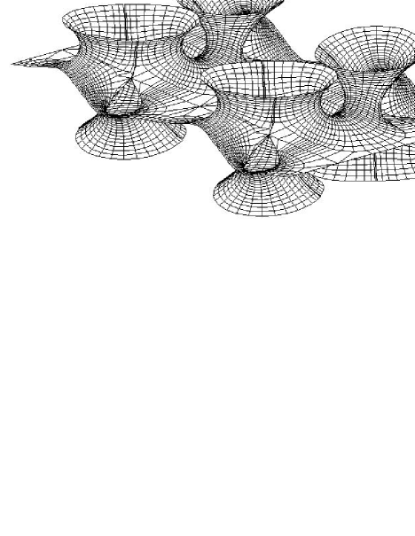
Figure 1: The surfaces ${\rm CL}_{\frac{\pi}{2}}$.

One can interpret $P$ as the Costa surface with its catenoidal ends kept, but the planar end replaced by $\partial P$. Point $S$ represents the “Costa-saddle”, where the lines meet. Of course, the spanned doubly periodic surface will have self-intersections, but they will occur only at the catenoidal ends. Let us consider $S$ as the origin of $\mathbb{R}^{3}$ and the segments of $P\setminus\partial P$ contained in $Ox_{1}$, $Ox_{2}$. Therefore, $Ox_{3}$ becomes the axis for both “top” and “bottom” catenoidal ends. Moreover, we consider that $x_{3}=x_{1}\wedge x_{2}$ and $Ox_{1}$ intersects only the straight segments of $\partial P$. By projecting $\partial P$ orthogonally onto $x_{3}=0$, one sees that $Q$ must be orthogonal to $Ox_{1,2}$. Otherwise, it would occur more self-intersections than just at the ends.

Figure 2: The rectangle $Q$.

From Figure 2 we notice that $Q$ and the ends can assume different ratios and logarithmic growths, respectively (see [5] for a definition). Therefore, the ${\rm CL}_{\frac{\pi}{2}}$ examples make a two-parameter family of surfaces. Let us take a generic member from this family. Consider its quotient by the translation group followed by a compactification of the four ends. We then get a topological compact surface denoted $\overline{M}$ (see Figure 3a). From this picture one easily sees that $\overline{M}$ has genus 3. The stretch $A-L-F-D-A$ generates the surface lines, whereas $A-E-A$ and $F-N-F$ generates the reflectional symmetry curves.

Let us now consider $\rho:\overline{M}\to\overline{M}$ as the involution corresponding to $180^{\circ}$ rotation about $Ox_{3}$. It fixes $L,D,TC,S,BC,TC^{\prime},S^{\prime}$ and $BC^{\prime}$, but interchanges $A,F$ and $E,N$. Hence, the Euler-Poincaré formula gives

$$\chi(\overline{M}/\rho)=\frac{\chi(\overline{M})}{2}+\frac{8}{2}=2.$$

Namely, $\overline{M}/\rho$ is topologically $S^{2}$, which admits the unique conformal structure $\hat{\mathbb{C}}=\mathbb{C}\cup\{\infty\}$ by Koebe’s theorem. Since $\rho$ is a branched covering, it induces a conformal structure on $\overline{M}$. This determines a meromorphic map $z:\overline{M}\to\hat{\mathbb{C}}$, and up to a Möbius transformation we choose $z(S)=0$, $z(A)=1$ and $z(S^{\prime})=\infty$. Rotation of $180^{\circ}$ about $A-L$ fixes $0$, $1$ and $\infty$. Therefore, the induced involution in $\hat{\mathbb{C}}$ is a reflection in the real line. Consequently, $z(A-L)\subset\mathbb{R}$. However, neither $S$ nor $S^{\prime}$ belong to $A-L$. This means that $z(A-L)=[1,\tilde{x}]$ for some $\tilde{x}>1$ or $z(A-L)=[x,1]$ for a certain $x<1$. Since $S-L$ is fixed by $180^{\circ}$-rotation about itself, and this fixes $S^{\prime}$, then $z(S-L)\subset\mathbb{R}$. This implies that $z(S)=0<z(L)<z(A)=1$ and so $z(L)=x$ with $0<x<1$.

That rotation of $S-L$ about itself also fixes $L$ and $D$, namely $0$, $x$, $\infty$ and $z(D)$. So, it induces $z\to\bar{z}$ in $\hat{\mathbb{C}}$. But it interchanges pairs $(A,F)$, $(E,N)$, $(TC,BC)$ and $(TC^{\prime},BC^{\prime})$, while $z(E)=z(N)$ by $\rho$. Therefore,

$$\bar{z}(N)=z(E),\hskip 4.33601pt{\rm which\hskip 4.33601ptimplies}\hskip 4.33601ptz(E)=z(N)\in\mathbb{R},$$ (1)

and

$$z(TC)=\bar{z}(BC),\hskip 4.33601pt\bar{z}(TC^{\prime})=z(BC^{\prime}).$$ (2)

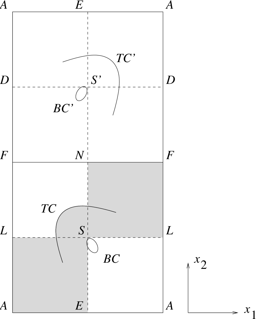
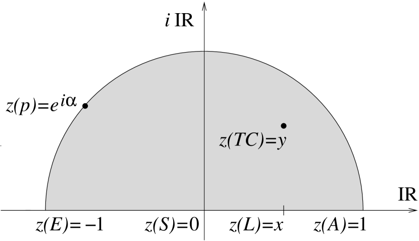
Figure 3: (a) The surface $\overline{M}$ with important points; (b) the map $z:\overline{M}\to\hat{\mathbb{C}}$.

Reflection in $A-E$ fixes $A,E,F,N$ and interchanges pairs $(TC,TC^{\prime})$, $(BC,BC^{\prime})$, $(S,S^{\prime})$ and $(L,D)$. This means, it fixes $1$ and interchanges $0,\infty$. Therefore, the induced involution in $\hat{\mathbb{C}}$ is given by $z\to 1/\overline{z}$, whence $z(D)=1/\bar{z}(L)=1/x$ and

$$z(TC)=1/\bar{z}(TC^{\prime}),\hskip 4.33601ptz(BC)=1/{z}(BC^{\prime}).$$ (3)

Observe that the fixed points of this involution belong to $S^{1}$. Therefore

$$z(E)=z(N)\in S^{1}.$$ (4)

From (1), (4) and the fact that $z(A)=1$ we get $z(E)=z(N)=-1$. Since rotation about $A-L$ does not fix $TC$, then $z(TC)=:y\in\mathbb{C}\setminus\mathbb{R}$. From (2) and (3) we get $z(BC)=\bar{y}$, $z(TC^{\prime})=1/\bar{y}$ and $z(BC^{\prime})=1/y$. The curves $A-E-A$ and $F-N-F$ are in planes parallel to $x_{2}=0$ and have highest and lowest points. Let $p,p^{\prime}$ and $q,q^{\prime}$ be such points on $A-E-A$ and $F-N-F$, respectively. Notice that $\measuredangle(A-E,A-L)=\pi/2$ and $A$ is not fixed by $\rho$, thus $\measuredangle(z(A-E),z(A-L))=\pi/2$. Since reflection in $A-E$ is given by $z\to 1/\bar{z}$, then $z(A-E)\subset S^{1}$. Without loss of generality we can take $Im\{y\}>0$, which implies $|y|<1$ and $z(p)=e^{i\alpha}$ for some $\alpha\in(0,\pi)$. Notice that $\rho$ interchanges $p$ with $q$, thus $z(q)=e^{i\alpha}$. Rotation about $S-E$ gives $z(p^{\prime})=\bar{z}(p)$ and $z(q^{\prime})=\bar{z}(q)$, hence $z(p^{\prime})=z(q^{\prime})=e^{-i\alpha}$. Figure 3b illustrates the map $z:\overline{M}\to\mathbb{C}$.

Since $\rho:\overline{M}\to\overline{M}$ is the hyperelliptic involution, it is easy to write down an algebraic equation for $\overline{M}$:

$$w^{2}=\frac{Z^{2}-2Re\{Y\}Z+|Y|^{2}}{(Z-X)(Z-2\cos\alpha)^{2}},$$ (5)

where $X=x+1/x$, $Y=y+1/y$ and $Z=z+1/z$ with $x\in(0,1),|y|<1,Im\{y\}>0$ and $\alpha\in(0,\pi)$. The values $0^{\pm 1},x^{\pm 1},y^{\pm 1}$ and $\bar{y}\,^{\pm 1}$ give exactly all branch points of $z$, each of order $1$. From Riemann-Hurwitz formula, $8/2-2+1=3$, which agrees with the expected genus of $\overline{M}$. Now suppose that $M$ is a complete minimal immersion of $\overline{M}\setminus\{TC,BC,TC^{\prime},BC^{\prime}\}$ in $\mathbb{R}^{3}$. For the Weierstraßdata $(g,dh)$, since $g$ is the stereographic projection of the unitary normal on $M$, based on Figures 1 and 3a we settle

$$g=icw,\text{ \ where \ }c>0.$$ (6)

From the sought after ends and regular points of $M$, $g$ determines all zeros and poles of $dh$, including their branch order. Therefore, we know that $S,S^{\prime},D,L,p$, $p^{\prime},q$ and $q^{\prime}$ are exactly the points where $dh$ vanishes, whereas it takes $\infty$ precisely at $TC,BC,TC^{\prime}$ and $BC^{\prime}$. By comparing $dh$ with $z$ and $dz$, we settle

$$dh=-\frac{i(Z-2\cos\alpha)dz/z}{Z^{2}-2Re\{Y\}Z+|Y|^{2}}.$$ (7)

Table (8) summarises the involutions of $\overline{M}$ and symmetries of $M$:

Symmetry Involution $$z$$

(8)

According to this table, $dh\cdot dg/g$ is real only on $A-E$, and purely imaginary otherwise. Hence, the sought after surfaces really have all the expected symmetry curves and lines.

4. Period Analysis

Figure 4 represents the fundamental piece $P$ of $M$ with open periods. There we consider the curve $\gamma:=S\to L\to A\to E\to S$.

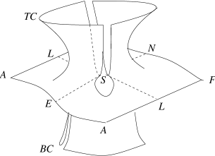
Figure 4: The fundamental piece with open periods.

For every closed curve in $\overline{M}\setminus\{TC,BC,TC^{\prime},BC^{\prime}\}$, one analyses the period vector $Re\oint\phi_{1,2,3}$. For instance, if such a curve is homotopic to $TC$ in $\overline{M}$, then it is homotopically $\rho(\gamma)\cup\gamma$. Hence, one must prove that $Re\int_{\gamma}\phi_{1,2,3}=0$. The same conclusion holds for $BC$, $TC^{\prime}$ and $BC^{\prime}$, after applying involutions of $\overline{M}$. For $A\to L\to F$, the period is zero on $Ox_{1,3}$ but non-zero on $Ox_{2}$, since it is taken to a line parallel to that axis, under the minimal immersion. Now, $A\to E\to A$ is in a plane parallel to $Ox_{1}x_{3}$, whence its period vanishes on $Ox_{2}$. If the period is zero on $\gamma$, we shall have $Re\int_{A\to E}\phi_{1}=Re\int_{L\to S}\phi_{1}\not=0$, for the latter is a straight segment in $M$. Finally, it is enough to prove that the period is zero on $\gamma$. Namely, the constant $c=c(x,y,\alpha)$ and $\alpha=\alpha(y)$ must satisfy the following three conditions:

$$\cos\alpha=\frac{\int_{0}^{\pi}\frac{\cos tdt}{4\cos^{2}t-4Re\{Y\}\cos t+|Y|^{2}}}{\int_{0}^{\pi}\frac{dt}{4\cos^{2}t-4Re\{Y\}\cos t+|Y|^{2}}};\hskip 4.33601ptc^{2}=c_{1}:=\frac{I_{1}+I_{2}}{-I_{3}+I_{4}};\hskip 4.33601ptc^{2}=c_{2}:=\frac{I_{5}-I_{6}}{I_{7}-I_{8}};$$ (9)

where $I_{1}=\int_{0}^{x}|dh/w|$, $I_{3}=\int_{0}^{x}|wdh|$, $I_{5}=\int_{-1}^{0}|dh/w|$, $I_{6}=\int_{x}^{1}|dh/w|$, $I_{7}=\int_{x}^{1}|wdh|$ and $I_{8}=\int_{-1}^{0}|wdh|$, for $z(t)=t$ varying in real intervals. Regarding $I_{2,4}$, $z(t)=e^{it}$ and $0\leq t\leq\pi$, so that $I_{2}=\int_{0}^{\pi}|dh/w|$ and $I_{4}=\int_{0}^{\pi}|wdh|$. Notice that $I_{2,4}$ remain invariant if one chooses $z(t)=e^{-it}$ instead. This fact will be used in the next section.

From (5) and (7), one clearly recognises the complexity of Equations (9). If we tried the intermediate value theorem, many cares would be necessary. For instance, one needs to survey the $(x,y)$-region where both denominators of $c_{1,2}$ do not vanish. Afterwards, positiveness must hold in a certain connected subregion, of which the boundary has points where $c_{1}-c_{2}$ changes sign close by. For Equations (9), the authors realised that these procedures were far too laborious and fruitless. In the next section, we apply the limit-method to solve (9), practically without computations.

5. Application of the Limit-Method

In order to apply the method explained in the Introduction, we shall first analyse the Weierstraßdata of $M=M_{x,y,\alpha}$. If one considers the function $z$ as a variable in the complex plane, one of the limits for $x\to 0$ will give the Weierstraßdata of the so-called $M_{\rm L_{b}}$-surfaces (see [15], p482). For this latter we have a solution of periods given by the transversal crossing of two graphs (see [15], pp486-9). Roughly saying, these are graphs of $xc_{1,2}$ at $x=0$, which means that the functions $c_{1,2}$ coincide for small $x>0$, at certain values of $y$ and $\alpha$, which will depend on $x$. Moreover, the crossing happens at positive values of $xc_{1,2}|_{x=0}$, so that $c^{2}$ is positive.

Take any $\lambda>1$ and $\rho\in(-\pi/2,0]$. If $x$ is sufficiently close to zero, the choice

$$\bar{y}(x):=\frac{xe^{i\rho}}{e^{i\rho}+i\lambda}$$ (10)

guarantees that $\bar{y}(x)$ belongs to the interior of $\mathcal{D}^{-}:=\{z\in\mathbb{C}:|z|\leq 1\leq 1-Im\{z\}\}$.

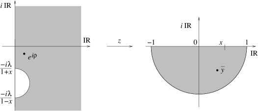
Figure 5: The map $z(\zeta)$.

Consider $C:=\sqrt{x\lambda}\cdot c$ and $K$ a compact set in the region $\mathcal{B}:=\{\zeta\in\hat{\mathbb{C}}:Re\{\zeta\}\geq 0\}\setminus\{-\lambda i,e^{i\rho}\}$. Soon we shall prove that $C^{2}$ has a finite positive limit, no matter which equation one takes from (9). Assume this for the moment and also take $C_{j}:=x\lambda\cdot c_{j}$, $j=1,2$. For $x$ sufficiently close to zero, the sector $\{\zeta\in\mathbb{C}:|\zeta+\frac{i\lambda}{1-x^{2}}|<\frac{\lambda x}{1-x^{2}}\}$ will be disjoint from $K$. Let $z:K\to\mathcal{D}^{-}$ be the map $z(\zeta)=\frac{x\zeta}{\zeta+i\lambda}$ and define $G(\zeta):=g\circ z(\zeta)$, $dH:=\frac{\lambda}{x}z^{*}dh$. Now fix any $\zeta\in K$. From (5), (6) and (7) we have

$$\lim_{x\to 0}G^{2}(\zeta)=\lim_{x\to 0}\frac{-C^{2}w^{2}(\zeta)}{x\lambda}=\frac{iC^{2}\zeta(\zeta-e^{i\rho})(\zeta+e^{-i\rho})}{(\zeta+i\lambda)^{2}};$$ (11)

$$\lim_{x\to 0}dH(\dot{\zeta})=\lim_{x\to 0}\frac{\lambda dh(\dot{\zeta})}{x}=\frac{d\zeta}{(\zeta-e^{i\rho})(\zeta+e^{-i\rho})}.$$ (12)

One readily recognises (11) and (12) as the Weierstraßdata of $M_{\rm L_{b}}$, up to $90^{\circ}$-rotation about the vertical axis (see [15], pp483-4). From this and (9), it easily follows that $\sqrt{\frac{\lambda^{3}}{x}}I_{1,5,6}$ and $\sqrt{\frac{\lambda}{x^{3}}}I_{3,7,8}$ will converge to the integrals in (13) and (22) of [15], pp486-8. Now, uniform convergence can be established by the following argument.

Notice that $I_{5}-I_{6}=\int_{\sigma}dh/w$, where $\sigma$ is homotopic to $\partial\mathcal{D}^{-}\setminus(0,x)$ in $\mathcal{D}^{-}\setminus\{\bar{y}\}$. Similarly, $I_{7}-I_{8}=\int_{\sigma}wdh$. A suitable choice of $K$ will guarantee that $(\{0\}\times i[0,+\infty])\cup\{z^{*}\sigma\}\subset K$. From [15], pp485-8, one sees that the corresponding limit-integrals share the same property. Convergence for $x$ approaching zero will then be uniform, because the integrals are well-defined on paths contained in $K$.

It remains to analyse $I_{2,4}$. In the sequel we prove that, for a curve $\zeta(t)$ homotopic to $\beta(t):=\frac{-i\lambda}{1-x^{2}}(1+xe^{it})$, $t\in[0,\pi]$, one has $\lower 5.5pt\hbox{${{\displaystyle\lim}\atop{}^{x\to 0}}$}\ {\sqrt{\frac{\lambda^{3}}{x}}}I_{2}=0$ and $\lower 5.5pt\hbox{${{\displaystyle\lim}\atop{}^{x\to 0}}$}\ {\sqrt{\frac{\lambda}{x^{3}}}}I_{4}=\frac{\lambda\pi}{f(\lambda)}$, where $f(\lambda)=\sqrt{\lambda(1+\lambda^{2}+2\lambda\sin\rho)}$. From this fact and the uniform convergence of the Weierstraßdata from $M_{x,y,\alpha}$ to $M_{\rm L_{b}}$ in $K$, it follows that $C_{1}$ and $C_{2}$ coincide at $x=0$ with the constants (13) and (22) of [15], pp486-8. Namely, $C_{1,2}$ are transversal in a neighbourhood of $x=0$. Therefore, $C_{1}=C_{2}$ (and consequently $c_{1}=c_{2}$) for $x$ close to zero, $\lambda=\lambda(x)$ with $\lambda(0)=\lambda_{\rho}$, and $\bar{y}(x)=xe^{i\rho}/(e^{i\rho}+i\lambda)$.

On $\beta(t)$, a careful computation shows that $\lower 5.5pt\hbox{${{\displaystyle\lim}\atop{}^{x\to 0}}$}\ {z(t)}=e^{-it}$. Therefore,

$$\lim_{x\to 0}\sqrt{x}\cdot|w|\biggl{|}_{\beta(t)}=\frac{|i\lambda+e^{i\rho}|}{2|\cos t-\cos\alpha|}$$ (13)

and

$$\lim_{x\to 0}\frac{|dh|}{x^{2}}\biggl{|}_{\beta(t)}=\frac{2|\cos t-\cos\alpha|dt}{|i\lambda+e^{i\rho}|^{2}}.$$ (14)

From (13) and (14) one readily sees that $\lower 5.5pt\hbox{${{\displaystyle\lim}\atop{}^{x\to 0}}$}\ {\sqrt{\frac{\lambda^{3}}{x}}}I_{2}=0$ and $\lower 5.5pt\hbox{${{\displaystyle\lim}\atop{}^{x\to 0}}$}\ {\sqrt{\frac{\lambda}{x^{3}}}}I_{4}=\lambda\pi/f(\lambda)$. This finally proves that Equations (9) have a simultaneous and positive solution on a curve $y(x,\lambda(x),\rho)$ and $\alpha=\alpha(y(x))$, for positive $x$ in a neighbourhood of zero.

6. Embeddedness of the Fundamental Piece

As mentioned in the Introduction, one can profit from the limit-method to prove embeddedness by arguments similar to [15], pp489-492. The convergences already studied in Section 5 will be now useful to simplify our task. There we proved the existence of a positive $\varepsilon$ and a curve $\bar{y}:(0,\varepsilon)\to\mathcal{D}^{-}$, for which the choice $c=c(x,y(x),\alpha(x))$ in (6) satisfies Equations (9). From now on, $c$ will always represent such a choice.

As a matter of fact, a free parameter $\rho$ can be chosen in $(-\pi/2,0]$, which establishes the curve $\lambda:(0,\varepsilon)\to(1,\infty)$, and $y$ is finally given by (10). By taking $z=\frac{x\zeta}{\zeta+i\lambda}$, $\zeta\in\mathcal{B}$ and $dH=\lambda dh/x$, when $x=0$ the constants $C_{1,2}$ from the previous section will close the periods of the surfaces in [15].

Choose any $x\in(0,\varepsilon)$ and consider the minimal immersion $X_{x}:\overline{M}\setminus z^{-1}(\{y^{\,\pm},\bar{y}^{\,\pm}\})\to\mathbb{R}^{3}$ defined by (5-7). Hence, $X_{x}$ restricted to $z^{-1}(\mathcal{D}^{-})$ can be viewed as a bivalent function $X_{x}:D^{-}\setminus\{\bar{y}\}\to\mathbb{R}^{3}$. Indeed, each branch $w$ of square root in (5) takes any point $q\in D^{-}\setminus\{\bar{y}\}$ to a pair of points in $\mathbb{R}^{3}$, say $X_{x}(q)^{+}$ and $X_{x}(q)^{-}$. Fix $X_{x}(0)$ as the origin, then one is the image of the other by 180^∘-rotation about $Ox_{3}$ (see Figure 6a). Moreover, for any closed curve homotopic to $\partial\mathcal{D}^{-}$, the period vector on it is zero, as proved in Section 5.

Consider the fundamental piece $P$ of $M$. Let $P^{-}$ be the image of $D^{-}\setminus\{\bar{y}\}$ in $\mathbb{R}^{3}$ under $X_{x}$, and $P^{+}$ the image in $\mathbb{R}^{3}$ of $P^{-}$ under 180^∘-rotation about either $X_{x}([0,x])$ or $X_{x}([-1,0])$. Therefore, $P=P^{-}\cup P^{+}$. The image of $\partial\mathcal{D}^{-}$ by $X_{x}$ is depicted in Figure 6b.

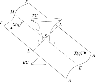
Figure 6: (a) The fundamental piece $P$; (b) the image of $\partial\mathcal{D}^{-}$ by $X_{x}$.

In Section 5 we defined the set $\mathcal{B}$. Let $\mathcal{K}$ be a compact subset of $\mathcal{B}$ such that $\mathcal{B}\setminus\mathcal{K}=V_{AE}\cup V_{BC}$, where $V_{AE}$ and $V_{BC}$ are connected neighbourhoods of $-i\lambda$ and $e^{i\rho}$, respectively. From (11) and (12), one sees that our data $(g,\lambda dh/x)$ converge uniformly on $\mathcal{K}$ to the Weierstraßpar of the embedded surface $M_{\rm L_{b}}$, with $\lower 5.5pt\hbox{${{\displaystyle\lim}\atop{}^{x\to 0}}$}\ \sqrt{x\lambda}c(x)=c_{\rm L_{b}}$ (see [15]). We denote its corresponding minimal embedding by $X_{0}$.

By [5] or [10], if $V_{BC}$ is small enough, then $X_{x}\big{|}_{V_{BC}}$ is the graph of

$$x_{3}(x_{1},x_{2})=\frac{\eta}{2}\ln(x_{1}^{2}+x_{2}^{2})+\mu+\frac{ax_{1}+bx_{2}}{x_{1}^{2}+x_{2}^{2}}+\mathcal{O}((x_{1}^{2}+x_{2}^{2})^{-1}),$$

where $\eta,\mu,a$ and $b$ are real numbers. This characterises $X_{x}\big{|}_{V_{BC}}$ as a catenoidal end. Since all the parameters vary continuously, $x\to 0$ implies that $X_{x}\big{|}_{V_{AE}}$ approaches a pair of Scherk ends, which are also graphs (see [16]). Thus we can choose $V_{AE}$ small enough for $X_{0}\big{|}_{V_{AE}}$ to be a graph. If $x$ is sufficiently close to zero, then the projection of $X_{x}\big{|}_{\partial V_{AE}}$ into $x_{3}=0$ will be a pair of simple closed curves $\mathcal{C}^{\pm}$, each one consisting of a regular arc and three segments, according to Figure 7. In fact, these curves determine two open regions in the plane, $R^{+}$ and $R^{-}$, bounded and simply connected.

Figure 7: Regions $R^{\pm}$ and curves $\mathcal{C}^{\pm}$.

For sufficiently small $V_{AE}$, $g(V_{AE})$ is contained in a half-sphere of $S^{2}$. This implies that $(x_{1},x_{2})\big{|}_{V_{AE}}$ is an immersion, namely into $R^{\pm}$ because $x_{2}$ is bounded for any $x\in(0,\varepsilon/2)$. Since $\partial R^{\pm}$ are the monotone curves $\mathcal{C}^{\pm}$, then $X_{x}\big{|}_{\partial V_{AE}}$ is a graph of $x_{3}$ as a function of $(x_{1},x_{2})$. The ends do not intersect for sufficiently small $V_{AE}$, $V_{BC}$ and $x$. Hence $X_{x}\big{|}_{V_{AE}}$, $X_{x}\big{|}_{V_{BC}}$ and $X_{x}\big{|}_{\mathcal{K}}$ are disjoint embeddings in $\mathbb{R}^{3}$.

$X_{0}\big{|}_{\mathcal{K}}$ is a compact embedded minimal surface with boundary in $\mathbb{R}^{3}$. Since the boundary has no self-intersections, then $X_{x}\big{|}_{\mathcal{K}}$ is still embedded for $x$ close enough to zero. Moreover, $X_{x}\big{|}_{\mathcal{K}}$ intersects neither $X_{x}\big{|}_{V_{AE}}$ nor $X_{x}\big{|}_{V_{BC}}$, otherwise there would be a ball in $\mathbb{R}^{3}$ containing the whole boundary of $X_{x}\big{|}_{\mathcal{K}}$, but not all the rest of it. This is impossible in the minimal case. Hence, the embedded pieces $X_{x}\big{|}_{V_{AE}}$, $X_{x}\big{|}_{V_{BC}}$ and $X_{x}\big{|}_{\mathcal{K}}$ make up a whole embedded minimal surface $X_{x}:\mathcal{B}\to\mathbb{R}^{3}$, for any $x$ sufficiently close to zero.

This extends to every $x$ in $(0,\varepsilon)$ by means of the maximum principle. Therefore, $P^{-}$ is embedded in $\mathbb{R}^{3}$, and since $P^{+}$ is its image under $180^{\circ}$ rotation around either $X_{x}([0,x])$ or $X_{x}([-1,0])$ of $P^{-}$, the whole piece $P$ has no self-intersections. The immersion is proper, so $P$ is embedded in $\mathbb{R}^{3}$.

7. Comments and Remarks

As we have just seen, the ${\rm CL}_{\frac{\pi}{2}}$-examples build a continuous two-parameter family of minimal surfaces. We claim that, for each example, both parameters control the $Q$-ratio and the logarithmic growth of the ends. From (7) and (10) it is easy to compute

$$Res(dh,z=\bar{y})=\frac{\bar{Y}-2\cos\alpha}{2(\bar{y}-1/\bar{y})Im\{Y\}}.$$ (15)

In Section 5 we proved that the fundamental piece has no periods. Consequently, $Re\{2\pi iRes(dh,z=\bar{y})\}=0$ and the following relation holds:

$$\cos\alpha=\frac{2Re\{y\}}{1+|y|^{2}}.$$ (16)

This means that the $y(x)$-curve matches (9) and (16). By substituting (16) in (15) we get

$$Res(dh,z=\bar{y})=\frac{1-|y|^{2}}{2Im\{Y\}}.$$ (17)

From (10) and (17) one easily gets $\lower 5.5pt\hbox{${{\displaystyle\lim}\atop{}^{x\to 0}}$}\ {\frac{\lambda}{x}Res(dh,z=\bar{y})}=\frac{1}{2}\sec\rho$. This is exactly the value in [15], p486. Of course, $x$ and $\rho$ act simultaneously for the logarithmic growth and the $Q$-ratio. In order to get parameters which would control each ratio separately, say $\ell$ and $\boldsymbol{q}$, one should invert the following system of equations:

$$\ell=\frac{1-|y(x,\rho)|^{2}}{2Im\{Y(x,\rho)\}}\hskip 4.33601pt\hskip 4.33601pt{\rm and}\hskip 4.33601pt\hskip 4.33601pt\boldsymbol{q}=\frac{I_{1}(x,\rho)+c^{2}(x,\rho)I_{3}(x,\rho)}{I_{6}(x,\rho)+c^{2}(x,\rho)I_{7}(x,\rho)}.$$

Let us now briefly discuss another limit-surface that could be used to obtain the ${\rm CL}_{\frac{\pi}{2}}$-examples. In [15], pp492-5, one studies the so-called $M_{\rm C_{b}}$-surfaces. If we let $x\to 1$, then

$$\lim_{x\to 1}g^{2}=\frac{-c^{2}(Z^{2}-2Re\{Y\}+|Y|^{2})}{(Z-2)(Z-2\cos\alpha)^{2}}$$ (18)

and

$$\lim_{x\to 1}dh=\frac{-i(Z-2\cos\alpha)dz/z}{Z^{2}-2Re\{Y\}+|Y|^{2}}.$$ (19)

From [15], p493, one readily recognises (18) and (19) as the Weierstraßdata of the surfaces $M_{\rm C_{b}}$. Moreover, $\lower 5.5pt\hbox{${{\displaystyle\lim}\atop{}^{x\to 1}}$}\ {2I_{6}}=0$ and $\lower 5.5pt\hbox{${{\displaystyle\lim}\atop{}^{x\to 1}}$}\ {2I_{7}}=\pi/|2-Y|$, namely $c_{1,2}$ coincide at $x=1$ with the corresponding López-Ros parameters (41) and (42) of [15]. Indeed,

$$I_{6}=\int_{x}^{1}|dh/w|=\frac{1}{\sqrt{x}}\int_{x}^{1}\frac{\sqrt{(x^{2}+1)t-t^{2}x-x}(t^{2}+1-2t\cos\alpha)^{2}dt}{\sqrt{t}[(t^{2}+1)^{2}-2Re\{Y\}(t^{3}+t)+|Y|^{2}t^{2}]^{3/2}}.$$

By means of the change $v=(x-t)/(x-1)$, it is clear that $\lower 5.5pt\hbox{${{\displaystyle\lim}\atop{}^{x\to 1}}$}\ {2I_{6}}=0$.

$$2I_{7}=2\int_{x}^{1}\frac{\sqrt{xt}\,dt}{\{(1-xt)(t-x)[(t^{2}+1)^{2}-2Re\{Y\}(t^{3}+t)+|Y|^{2}t^{2}]\}^{1/2}}.$$

After applying the change $t=x+(1-x^{2})u^{2}$, it follows that

$$2I_{7}=4\sqrt{x}\int_{0}^{\frac{1}{\sqrt{1+x}}}\frac{\sqrt{(1-x^{2})u^{2}+x}\,du}{\{(1-xu^{2})[(t^{2}+1)^{2}-2Re\{Y\}(t^{3}+t)+|Y|^{2}t^{2}]\}^{1/2}}.$$

Therefore,

$$\lim_{x\to 1}2I_{7}=4\int_{0}^{\frac{1}{\sqrt{2}}}\frac{du}{[(1-u^{2})(4-4Re\{Y\}+|Y|^{2})]^{1/2}}=\frac{\pi}{|2-Y|}.$$

In [15], p494, one gets a whole solution curve $(\alpha(t),y(t))$ on which the equality $c_{1}|_{x=1}=c_{2}|_{x=1}$ holds. This curve is obtained by a transversal crossing of graphs on an open subset of $\mathbb{R}^{2}$. The limit-method then gives functions $\alpha(t,x)$ and $y(t,x)$, for $x\in(1-\varepsilon,1)$, which correspond to a simultaneous and positive solution of (9).

References

[1] Barbosa, J.L., do Carmo, M.P. and Eschenburg, J., Stability of hypersurfaces of constant mean curvature in Riemannian manifolds, Math. Z. 197 (1988), 1, 123–138.
[2] Costa, C.J. Example of a complete minimal immersion in of genus one and three embedded ends. Bol. Soc. Brasil. Mat. 15 (1984), 1-2, 47–54.
[3] Chen, C.C. and Gackstatter, F. Elliptische und hyperelliptische Funktionen und vollständige Minimalflächen vom Enneperschen Typ. Math. Ann. 259 (1982), 3, 359–369.
[4] M. Callahan, D. Hoffman and W. H. Meeks. Embedded minimal surfaces with an infinite number of ends. Inventiones Math., Vol.96, 1989, 459-505.
[5] Hoffman, D. and Karcher, H., Complete embedded minimal surfaces of finite total curvature, Encyclopaedia Math. Sci. 90 (1997) 5-93.
[6] Kapouleas, N., Complete embedded minimal surfaces of finite total curvature, J. Differential Geom. 47 (1997), 1, 95–169.
[7] Karcher, H.: Construction of minimal surfaces, Surveys in geometry. University of Tokyo (1989) 1–96 and Lecture Notes 12 (1989), SFB256, Bonn.
[8] Lübeck, K.R.M. Método-Limite para solução de períodos em superfícies mínimas, doctoral thesis, Campinas 2007.
[9] F.J. López & F. Martín, Complete minimal surfaces in , Publ. Mat. 43 (1999) 341–449.
[10] Miyaoka, R. and Sato, K., On complete minimal surfaces whose Gauss map misses two points, Arch. Math. 63 (1994) 565-576.
[11] J.C.C. Nitsche, Lectures on minimal surfaces, Cambridge University Press, Cambridge (1989).
[12] R. Osserman, A survey of minimal surfaces, Dover, New York, 2nd ed (1986).
[13] Ramos Batista, V.: Construction of new complete minimal surfaces in based on the Costa surface, Doctoral thesis, University of Bonn (2000).
[14] Ramos Batista, V.: The doubly periodic Costa surfaces, Math. Z. 240 (2002) 549-577.
[15] Ramos Batista, V.: Singly periodic Costa surfaces, J. London Math. Soc. (2) 72 (2005) 478-496.
[16] Traizet, M. Construction de surfaces minimales en recollant des surfaces de Scherk. Ann. Inst. Fourier 46 (1996), 1385-1442.
[17] Traizet, M.: Adding handles to Riemann’s minimal surfaces. J. Inst. Math. Jussieu 1 (2002), 1, 145–174.
[18] Traizet, M.: An embedded minimal surface with no symmetries. J. Differential Geom. 60 (2002), 1, 103–153.
[19] Weber, M.: The Genus One Helicoid is Embedded, Habilitation Thesis, Bonn 2000.
[20] Weber, M.: A Teichmüller theoretical construction of high genus singly periodic minimal surfaces invariant under a translation. Manuscripta Math. 101 (2000), 2, 125–142.