Entanglement spectrum in one-dimensional systems
Abstract
We derive the distribution of eigenvalues of the reduced density matrix of a block of length in a one-dimensional system in the scaling regime. The resulting “entanglement spectrum” is described by a universal scaling function depending only on the central charge of the underlying conformal field theory. This prediction is checked against exact results for the XX chain. We also show how the entanglement gap closes when is large.
The interest in quantifying the entanglement in extended quantum systems has been growing in recent times at an impressive rate, mainly because of its ability to detect the scaling behavior in proximity of quantum critical points (see e.g. Refs. rev as reviews). Among the various measures, the so-called entanglement entropy has by far been the most studied. By partitioning an extended quantum system into two blocks, the entanglement entropy is defined as the von Neumann entropy of the reduced density matrix of one of the two blocks. The success of this quantity can be understood because it is a single number able to capture the main features of the scaling behavior. In fact, in one-dimensional (1D) critical ground-states, when the block is a segment of length in an infinite system, the entanglement entropy diverges with the logarithm of the block size as Holzhey ; Vidal ; cc-04
| (1) |
where is the central charge of the associated conformal field theory (CFT) and a non-universal constant. Away from the critical point, saturates to a constant value Vidal proportional to the logarithm of the correlation length cc-04 .
However, the reduced density matrix (at least in principle) contains more information than the entanglement entropy. This information should be encoded in the full spectrum of the reduced density matrix, which we shortly call “entanglement spectrum”, following Ref. lh-08 . In this letter we calculate the entanglement spectrum for 1D systems in the scaling regime, i.e. at or close to a quantum critical point. The study of the distribution of eigenvalues provides clearly a deeper theoretical understanding of entanglement and correlations in extended systems, but not only. Indeed, all numerical algorithms based on the so-called matrix product states (among which density matrix renormalization group dmrg is the best known) give as first output a truncated spectrum of the reduced density matrix and from this all the other quantities are derived. Consequently, the knowledge of some scaling properties of this distribution provides an optimal check for the convergence and the accuracy of the numerics and could be used for putting accurate bounds on the efficiency of these methods as already done from other quantities in Refs. acc .
The scaling behavior of the entanglement spectrum can be related to the properties of the moments of the reduced density matrix: , where are the eigenvalues of . In the scaling regime, can be written as
| (2) |
where is a non-universal constant and is the relevant length in the considered regime. For example, equals the length block if is part of an infinite gapless system Holzhey ; cc-04 , if is in a finite gapless system of length , and cc-04 if the system is gapped [valid when the correlation length (the inverse mass gap) is large, but smaller than all the other lengths like ]. Everywhere stands for the scale setting the microscopic length, e.g. the lattice spacing. The same dependence is found in the case of open systems (the exponent of in Eq. (2) halves and so does cc-04 ) and when consists of more disjoint intervals cc-04 and also in some non-equilibrium situations neq . For practical reasons, it is convenient to write
| (3) |
where by simple inspection is related to the maximum eigenvalue: , as well known singcopy .
In order to characterize the entanglement spectrum, we define the distribution of eigenvalues , which is normalized to , where is the dimension of the local Hilbert space, e.g. for spin systems. We determine this distribution for a 1D system in the scaling regime where Eq. (2) applies. The only assumption in what follows is that the -dependence of the non-universal part of can be ignored, i.e. that we can write , with a constant function (i.e. the effect of is to replace the lengths appearing in with the dimensionless quantity ). A priori this can appear as a very crude approximation, but it is not the case. For the gapless XX chain, is known analytically jk-04 , and it is easy to show that varies less then 1% as soon as . Physically, this is equivalent to stating that the main contribution of is to set the microscopic length to be used in the continuum description in terms of the lattice one. We will check a posteriori for the XX chain that the result obtained ignoring describes accurately the actual entanglement spectrum when is large. A very precise numerical determination of for the XXZ chain with ccn-08 shows that the same scenario is true on the full critical line of the model. In few other cases is also known ch-05 ; ccd-07 ; fik-08 and similar properties can be found.
Thus, ignoring temporarily , we will compute the entanglement spectrum, using the simple observation that , with
| (4) |
Here, has an imaginary part when only on the support of , due to the pole in the r.h.s. of (4). The calculation of is straightforward:
| (5) |
where is the polylogarithm function, which is analytic on the complex plane, with a cut on the real axis for (that once again is just ). The discontinuity along the cut is given by for . The sum can be explictly done and we end up with
| (6) | |||||
where the delta peak comes from the contribution of in (5) and stands for the modified Bessel function of the first kind. In this derivation, only with positive integers enter. For these values (as we already discussed) in general does not vary significantly. This gives an argument that explains why Eq. (6) works well for large enough in the following calculations for the XX model and why the same is expected in general.
can also be obtained by considering the inverse Laplace transform of in the variable . Using standard results Eq. (6) is easily recovered. We preferred to give the previous derivation because it highlights the role played by positive integer , where can be ignored. Conversely the inverse Laplace transform requires an integral on the complex plane, over a contour where there is less control on the values of that are contributing relevantly. We noticed this because numerical inverse Laplace transform could be done in principle in more complicated cases (like those in Refs. jk-04 ; ccn-08 ; ch-05 ; ccd-07 ; fik-08 ) where the previous analytic reasoning does not work.
Let us discuss now the main properties of :
(i) The mean number of eigenvalues larger than a given is
| (7) |
Note that for , diverges, as it should, because in the continuum the number of eigenvalues is infinite. In the lattice models, this can be regularized by the finite number of degrees of freedom (as e.g. in spin chains), but not always (e.g. bosons have always infinitely many eigenvalues).
(ii)The normalization corresponds to , and follows directly from Eq. (6).
(iii) The entanglement entropy is given by
| (8) |
reproducing the result that the single copy entanglement equals one-half of the entanglement entropy singcopy .
(iv) Majorization is a relation between two probability distributions and whose elements are ordered (and similarly for ): it is said that majorizes if for any and . It has been argued, observed numerically and in some instances proven analytically, that with increasing the resulting distribution of eigenvalues is majorized by the ones at smaller scaling lengths maj ; zbfs-06 (sometimes this is referred to as majorization along renormalization group flow). From the previous result it is straightforward that majorization holds in the scaling regime when Eq. (6) for applies. In fact, we have
| (9) |
which, at fixed , is a monotonous function of (that is a monotonous function of ). This proves majorization in a very easy way. It is also simple to check majorization directly by making the numerical integral at fixed and varying .

We now compare the scaling function for the entanglement spectrum with the eigenvalues of lattice models, in order to show its predictivity and to highlight its limits. As a prototype of lattice models we consider the gapless XX chain defined by the Hamiltonian
| (10) |
where are the Pauli matrices at site . The reduced density matrix of a block of contiguous spins in an infinite chain (so, among the cases of before, this corresponds to ) can be obtained by exploiting the mapping to free fermions pesc ; Vidal :
| (11) |
where are spinless fermion annihilation operators, and
| (12) |

Calculating the eigenvalues of the matrix requires only the diagonalization of an matrix. In terms of the , the eigenvalues of the reduced density matrix are the products
| (13) |
where is a subset of and the complement. While it is possible to obtain all the up to very large , making all of the products to obtain the full spectrum requires far too much memory on a personal computer. Thus we calculate the full eigenvalue spectrum only up to (which corresponds to almost millions of eigenvalues), and for larger we truncated the fermionic spectrum to modes (i.e. we diagonalize the matrix finding all the , but in the products we do not vary the eigenvalues that are closer to or and generate the smaller ). This reproduces in the exact order the first few thousands eigenvalues, to which we limit our analysis in the truncated cases.
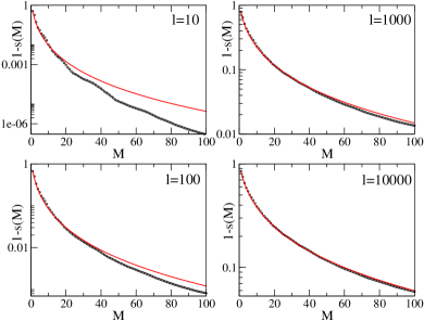
We start this analysis from the check of the “sumrule” given by Eq. (9). In Fig. 1 we report minus the sum of the first (up to ) eigenvalues for . It is evident that increasing the sum is well described by Eq. (9) for larger and larger values of . The (negative) deviations from the CFT take place at a value of that roughly scales like and they are obviously due to lattice effects, because the sum rule must be saturated by a finite sum up to that cutoffs the integral of the continuum limit.

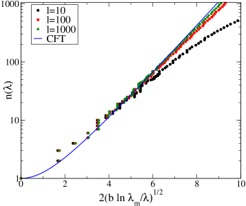
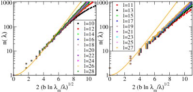
A stronger test of our predictions is provided by Eq. (7) that gives the total number of eigenvalues between and . This formula provides the natural scaling variable . Once is determined from the numerics, is just given by , independently from any other detail of the model under consideration and, more surprisingly, it is also independent from the model itself. Instead of plotting the number of eigenvalues larger than a given , we prefer to show the inverse function of that is the value of the -th eigenvalue. In addition to represent , this also has the advantage of giving information about the degeneracy of all eigenvalues, as the number of points at the same position on the horizontal axis. For this function is shown in Fig. 2 and compared with in Eq. (7). It is evident that when the spectrum becomes almost continuous, it is well described by the CFT prediction up to a given (i.e. a given ). Increasing the number of eigenvalues described by Eq. (7) increases and at , approximately thousands eigenvalues fall on the CFT scaling curve. The negative deviations for eigenvalues smaller than are due to lattice effects as in the previous case of the partial sumrule. The degeneracies of the eigenvalues are not reproduced by our approach. In Fig. 3 we plot the entanglement spectrum for all from to in order to show both finite-size and parity effects. When is odd (a case rarely considered in the literature) the approach to the asymptotic scaling is much slower. This can be understood because of the double degeneracy of all the eigenvalues (included the largest), which moves a large weight toward that, because of the sumrule, must be compensated by a smaller weight at large (i.e. small eigenvalues).
There is a final interesting feature that is clearly visible in Figs. 2 and 3. When plotting in terms of , the first few eigenvalues do not change their positions with changing . The logarithms of these discrete eigenvalues result to be equispaced, i.e.
| (14) |
where and are indices referring to two non-degenerate consecutive eigenvalues and is a constant that is different for even and odd (and we used and ). When , this simple formula tells us how the gap between the first and the second eigenvalues closes when increasing , which, following Ref. lh-08 , we call ”entanglement gap”. This scaling of the discrete part of the spectrum can be related to an old result about the scaling of the eigenvalues of the corner transfer matrix pt-87 . In fact, because is almost independent of , for this part of the spectrum the result should be the same as that of a segment in a system of length . In this case the reduced transfer matrix can be seen as the fourth power of a corner transfer matrix cc-04 (of angle ), for which the analogous of Eq. (14) has been derived from CFT pt-87 . Using this correspondence the asymptotic behavior of for gapped systems has been already derived in Ref. jap . However our result goes far beyond, explaining also the reason of such a simple result.
In conclusions, the main result of this letter is the analytic derivation of the universal entanglement spectrum for 1D models in the scaling regime, given by Eq. (6). This turns out to depend only on the central charge of the underlying conformal field theory. We found that Eq. (6) describes accurately the continuum part of the spectrum of the XX chain for large enough , and is expected to work for any model at or close to a quantum critical point. This can be seen as a surprise because it means that the continuum part of the entanglement spectrum does not contain more information than the entanglement entropy that is just one possible average over the spectrum. The reason for this (maybe unexpected) result can be traced back to the fact that conformal invariance in 1D is so strong that it fixes completely the shape of the full spectrum, leaving only one parameter (the central charge) free. Such parameter can be fixed by of a single “measure” like the entanglement entropy, the largest eigenvalue, etc.
Oppositely, the discrete part of the spectrum is only reproduced in average by Eq. (6). As a consequence, the location and the degeneracies of the low-lying eigenvalues of the reduced density matrix can still be a tool for extracting further universal information on the model under investigation that could not be captured by the entanglement entropy. For example, it is known that the degeneracies of eigenvalues of the isotropic Heisenberg antiferromagnetic chain are larger than the XXZ ones (because of the larger symmetry), but they all have and so the same continuum part of the spectrum. A careful study of these issues is needed, but it goes far beyond the goals of this letter.
Acknowledgments. This work started from a discussion with J. Cardy. We thank L. Tagliacozzo for pointing out the important Ref. pt-87 . We thank J. Cardy, A. Celi, S. Iblisdir, J. I. Latorre, B. Nienhuis, and L. Tagliacozzo for stimulating discussions. PC benefited of a travel grant from ESF (INSTANS activity).
References
- (1) L. Amico et al., Rev. Mod. Phys. 80, 517 (2008); J. Cardy, Eur. Phys. J. B, to appear.
- (2) C. Holzhey, F. Larsen, and F. Wilczek, Nucl. Phys. B 424, 443 (1994).
- (3) G. Vidal et al., Phys. Rev. Lett. 90, 227902 (2003); J. I. Latorre et al., Quant. Inf. and Comp. 4, 048 (2004).
- (4) P. Calabrese and J. Cardy, J. Stat. Mech. P06002 (2004); Int. J. Quant. Inf. 4, 429 (2006).
- (5) H. Li and F. D. M. Haldane, Phys. Rev. Lett. 101, 010504 (2008).
- (6) S. White, Phys. Rev. Lett. 69, 2863 (1992); U. Schollwoeck, Rev. Mod. Phys. 77, 259 (2005).
- (7) N. Schuch et al., Phys. Rev. Lett. 100, 030504 (2008); D. Perez-Garcia et al., Quantum Inf. Comput. 7, 401 (2007); L. Tagliacozzo et al., Phys. Rev. B 78, 024410 (2008).
- (8) P. Calabrese and J. Cardy, J. Stat. Mech. P04010 (2005); J. Stat. Mech. P10004 (2007).
- (9) J. Eisert and M. Cramer, Phys. Rev. A 72, 042112 (2005); I. Peschel and J. Zhao, J. Stat. Mech. P11002 (2005); R. Orus et al., Phys. Rev. A 73, 060303 (2006).
- (10) B.-Q. Jin, V. E. Korepin, J. Stat. Phys. 116, 79 (2004).
- (11) P. Calabrese, M. Campostrini, B. Nienhuis, to appear.
- (12) H. Casini and M. Huerta, J. Stat. Mech. P05012 (2005); H. Casini et al., J. Stat. Mech. P05007 (2005) .
- (13) J. L. Cardy et al., J. Stat. Phys. 130, 129 (2008).
- (14) F. Franchini et al., J. Phys. A 41, 025302 (2008).
- (15) J. I. Latorre et al., Phys. Rev. A 71, 034301 (2005); R. Orus, Phys. Rev. A 71, 052327 (2005); 73, 019904(E) (2006).
- (16) H.-Q. Zhou et al., Phys. Rev. A 74, 050305(R) (2006).
- (17) I. Peschel, J. Stat. Mech. P06004 (2004); I. Peschel, J. Phys. A 36, L205 (2003); M.-C. Chung and I. Peschel, Phys. Rev. B 64, 064412 (2001); I. Peschel et al., Ann. Physik (Leipzig) 8, 153 (1999).
- (18) I. Peschel and T. T. Truong, Z. Phys. B 69, 385 (1987).
- (19) K. Okunishi et al., Phys. Rev. E 59, R6227 (1999).