The high temperature Ising model
on the triangular lattice
is a critical percolation model

Abstract

The Ising model at inverse temperature $\beta$ and zero external field can be obtained via the Fortuin-Kasteleyn (FK) random-cluster model with $q=2$ and density of open edges $p=1-e^{-\beta}$ by assigning spin $+1$ or $-1$ to each vertex in such a way that (1) all the vertices in the same FK cluster get the same spin and (2) $+1$ and $-1$ have equal probability.

We generalize the above procedure by assigning spin $+1$ with probability $r$ and $-1$ with probability $1-r$, with $r\in[0,1]$, while keeping condition (1). For fixed $\beta$, this generates a dependent (spin) percolation model with parameter $r$. We show that, on the triangular lattice and for $\beta<\beta_{c}$, this model has a percolation phase transition at $r=1/2$, corresponding to the Ising model. This sheds some light on the conjecture that the high temperature Ising model on the triangular lattice is in the percolation universality class and that its scaling limit can be described in terms of SLE₆.

We also prove uniqueness of the infinite $+1$ cluster for $r>1/2$, sharpness of the percolation phase transition (by showing exponential decay of the cluster size distribution for $r<1/2$), and continuity of the percolation function for all $r\in[0,1]$.

Keywords: Ising model, random-cluster measures, dependent percolation, DaC models, fractional fuzzy Potts model, sharp phase transition, duality, $p_{c}=1/2$
AMS 2000 Subject Classification: 60K35, 82B43, 82B20

1 Introduction and motivation

If one considers the percolation properties of spin clusters, the high temperature ($\beta<\beta_{c}$) Ising model on the triangular lattice $\mathbb{T}$ with no external field is believed to show critical behaviour and to be in the universality class of Bernoulli (independent) percolation. One way to understand the conjecture is in terms of the renormalization group: one expects the high temperature phase of the Ising model to be in the basin of attraction of the (stable) infinite temperature fixed point, which in the case of the triangular lattice (but not of other lattices) corresponds to critical site percolation.

The conjecture can also be cast in the language of the $O(n)$ model. Indeed, the high temperature phase of the zero field Ising model on $\mathbb{T}$ falls in the so-called dense phase of the $O(n)$ model with $n=1$, which is believed to show critical behaviour and to be driven, under the action of the renormalization group, to a stable fixed point corresponding, once again, to critical percolation. Rephrased in the language of scaling limits, the conjecture can be expressed in terms of convergence of certain interfaces to SLE₆, and appears in several places (see, e.g., [24, 30, 31, 2]), often as part of a larger conjecture about the $O(n)$ model.

Motivated by the above considerations, in this paper we show that, for any fixed inverse temperature $\beta<\beta_{c}$, the zero field Ising model on $\mathbb{T}$ corresponds to the critical point of a dependent percolation model. To do that, we generalize the FK random-cluster representation of the Ising model, obtaining a site percolation model with parameter $r\in[0,1]$ which reduces to the Ising model for $r=1/2$. We then show that the new percolation model has a (sharp) percolation phase transition at $r=1/2$.

It will be clear from its definition that in the new percolation model the states of different sites are not independent, but that correlations decay exponentially with the distance. As a consequence, we can now view the conjecture about the high temperature Ising model on the triangular lattice as a particular instance of another general conjecture that has to do with percolation only, namely that the scaling limit of a (two-dimensional) percolation model exists and is independent of the particular model, as long as the correlations in the probability measure decay fast enough (see, e.g., [12]). Such a result has been proved for a few specific models of dependent percolation (see [11, 10, 8, 9, 5]).

It is interesting to notice that the Ising model corresponds to the self-dual point of the new percolation model. Therefore, our result also shows that for that model the self-dual and the critical point coincide, in accordance with a very natural principle which is believed to be valid in great generality, but which has been verified only in a handful of cases, including bond percolation on the square lattice [26], site percolation (see [27]) and the Divide and Colour (DaC) model [2] on the triangular lattice, and Voronoi percolation [6]. The same priciple should apply to other interesting models, such as the random-cluster model (where it is known for $q=1$, corresponding to percolation, and $q=2$, corresponding to the Ising model — see [16]), other DaC models (see [2], and in particular Conjecture 1.7 there) and “confetti percolation” (see Problem 5 in [3]).

In our analysis we make substantial use of a result by Higuchi, who has extensively studied the percolation properties of the two-dimensional Ising model (see [19, 20, 21, 22, 23]).

2 Main results

We work on the triangular lattice $\mathbb{T}$ with vertex set $\mathcal{V}_{\mathbb{T}}$ and edge set $\mathcal{E}_{\mathbb{T}}$, and denote the unique Ising Gibbs measure on $\mathbb{T}$ at inverse temperature $\beta<\beta_{c}$ and zero external field by $\mu_{\beta}$.

The random-cluster measure $\nu_{p,q}$ on edge configurations $\eta\in\{0,1\}^{\mathcal{E}_{\mathbb{T}}}$ (with the usual $\sigma$-field generated by cylinder events) is characterized by two parameters satisfying $0\leq p\leq 1$ and $q>0$ (see [16] for the definition and some background). We call an edge $e\in\mathcal{E}_{\mathbb{T}}$ open if $\eta(e)=1$, and closed otherwise. The maximal connected components of the graph obtained by removing all the closed edges from $\mathbb{T}$ are called FK clusters.

For fixed $q$, the random-cluster measure has a percolation phase transition at some $0<p_{c}(q)<1$, and with probability one all FK clusters are finite if $p<p_{c}(q)$. When $q=2$, one can generate an Ising spin configuration $\sigma\in\{+1,-1\}^{\mathcal{V}_{\mathbb{T}}}$ distributed according to $\mu_{\beta}$, $\beta<\beta_{c}$, by drawing an edge configuration according to $\nu_{p,2}$ with $p=1-e^{-\beta}$ and assigning spin $+1$ or $-1$ to each vertex of $\mathbb{T}$ in such a way that (1) all the vertices in the same FK cluster get the same spin and (2) $+1$ and $-1$ have equal probability. Note that $\beta<\beta_{c}$ implies $p=1-e^{-\beta}<p_{c}(2)$, so that the FK clusters are all finite with probability one.

From now on, unless otherwise stated, we will always assume that $q=2$. We generalize the above procedure by assigning spin $+1$ with probability $r$ and $-1$ with probability $1-r$, with $r\in[0,1]$, while keeping condition (1). For fixed $\beta$, this generates a dependent (spin) percolation model with parameter $r$, whose measure we denote by ${\mathbb{P}}_{\beta,r}$. Clearly, the spin marginal of ${\mathbb{P}}_{\beta,1/2}$ coincides with $\mu_{\beta}$. Note also that ${\mathbb{P}}_{0,1/2}$ (equivalently, $\mu_{0}$) is a product measure and corresponds to critical site percolation on $\mathbb{T}$. As soon as $\beta>0$, however, the spins are correlated. Nonetheless, the exponential decay of the FK cluster size distribution when $\beta<\beta_{c}$ (see [16]) immediately implies the exponential decay of correlations in the measure ${\mathbb{P}}_{\beta,r}$.

We call a maximal connected subset $V$ of ${\mathcal{V}_{\mathbb{T}}}$ such that all vertices in $V$ have the same spin a spin cluster. If the spins in $V$ are all $+1$ (respectively, $-1$), we call $V$ a ($+$)-cluster (resp., a ($-$)-cluster). Our aim is to study the percolation properties of spin clusters. We denote by $\Theta(\beta,r)$ the $\mathbb{P}_{\beta,r}$-probability that a given vertex of the triangular lattice is contained in an infinite ($+$)-cluster, and define $r_{c}(\beta):=\sup\{r:\Theta(\beta,r)=0\}$. By the size of a cluster we mean the number of vertices in the cluster. The main result of this paper is the following theorem where, due to the $+/-$ symmetry of the model, we focus without loss of generality on the behaviour of ($+$)-clusters.

Theorem 2.1.

For all $\beta<\beta_{c}$, $r_{c}(\beta)=1/2$. Moreover,

• If $r<1/2$, the distribution of the size of the ($+$)-cluster of the origin has an exponentially decaying tail.

• If $r=1/2$, $\Theta(\beta,1/2)=0$ and the mean size of the ($+$)-cluster of the origin is infinite.

• If $r>1/2$, there exists a.s. a unique infinite ($+$)-cluster.

Note that $r=1/2$ is clearly the self-dual point of ${\mathbb{P}}_{\beta,r}$. Thus, Theorem 2.1 implies that the critical point of the model coincides with its self-dual point. We remark that one can obtain a polynomial lower bound for the tail distribution of the ($+$)-cluster of the origin at $r=1/2$ by using elementary duality arguments only, see [17], p. 15.

Since the phase transition described in Theorem 2.1 is continuous, one may expect continuity of the percolation function $\Theta(\beta,r)$. Indeed, this can be proved by standard methods.

Theorem 2.2.

For each $\beta<\beta_{c}$, $\Theta(\beta,r)$ is a continuous function of $r\in[0,1]$.

It is worth remarking that ${\mathbb{P}}_{\beta,r}$ belongs to a family of measures that can be obtained via a two step procedure: first partition the vertices of a lattice into clusters according to some rule, then assign spin values (or colours) to the vertices with some probability, making sure that all vertices in the same cluster get the same colour. We call such measures Divide and Colour (DaC) models. The first DaC model was introduced by Häggström [18], and its phase transition is studied in detail in [2]. DaC models can be considered as natural dependent percolation models. They are relatively simple, yet their analysis is considerably more complicated than that of Bernoulli percolation (see, e.g., the present paper and [2]), and requires new techniques that may be useful in studying other dependent models.

A brief outline of the paper is given as follows. In Section 3, we introduce some more definitions and notation, and we collect results which are either known or can be proved by standard methods, including a result by Higuchi [22] about the Ising model. We shall use them later, together with the standard Edwards-Sokal coupling [13] and results described in Section 4, which contains some technical lemmas and an overview of the main step in the proof of Theorem 2.1. In Section 5, we prove Theorems 2.1 and 2.2.

3 Preliminaries

3.1 Notation and definitions

In order to define a concrete coordinate system in the triangular lattice $\mathbb{T}$, we embed $\mathbb{T}$ in ${\mathbb{R}}^{2}$ as in Figure 1, so that its set of vertices $\mathcal{V}_{\mathbb{T}}$ consists of the intersections of the lines $y=-\hskip 0.85355pt\sqrt{3}\hskip 1.42271ptx+\sqrt{3}\hskip 1.42271ptk$ and $y=\frac{\sqrt{3}}{2}\hskip 1.42271pt\ell$ for $k,\ell\in\mathbb{Z}$, and denote the elements of $\mathcal{V}_{\mathbb{T}}$ by $(k,\ell)$. We call two vertices in $\mathcal{V}_{\mathbb{T}}$ adjacent if their Euclidean distance is 1, and define the edge set $\mathcal{E}_{\mathbb{T}}$ by $\mathcal{E}_{\mathbb{T}}=\{(v,w):v$ and $w$ are adjacent$\}$.

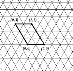
Figure 1: Portion of the triangular lattice $\mathbb{T}$. The heavy segments are the sides of the parallelogram $S_{2,3}=[0,2]\times[0,3]$.

The state space of our configurations is denoted by $\Omega:=\Omega_{D}\times\Omega_{C}$, where $\Omega_{D}=\{0,1\}^{\mathcal{E}_{\mathbb{T}}}$ is the set of random-cluster realisations, and $\Omega_{C}=\{-1,+1\}^{\mathcal{V}_{\mathbb{T}}}$ corresponds to the spin configurations. The probability measure $\mathbb{P}_{\beta,r}$ is the measure (on the usual $\sigma$-algebra on $\Omega$) obtained by the procedure described in Section 2; we denote the expectation with respect to $\mathbb{P}_{\beta,r}$ with $\mathbb{E}_{\beta,r}$.

We introduce the set $\tilde{\Omega}\subset\Omega$ as the set of configurations such that vertices in the same FK cluster have the same spin, and we equip $\tilde{\Omega}$ with a partial order, which depends on the spins only, as follows. For $\omega_{1}=(\eta_{1},\sigma_{1}),\omega_{2}=(\eta_{2},\sigma_{2})\in\tilde{\Omega}$ we say that $\omega_{1}\geq\omega_{2}$ if $\sigma_{1}(x)\geq\sigma_{2}(x)$ holds for every $x\in\mathbb{T}$. All the configurations are implicitly assumed to be in $\tilde{\Omega}$. We call an event $A\subset\tilde{\Omega}$ increasing if $\omega\in A$ and $\omega^{\prime}\geq\omega$ implies $\omega^{\prime}\in A$. $A$ is a decreasing event if $A^{c}$ is increasing.

We call a sequence $(x_{0},x_{1},\ldots,x_{n})$ of vertices in $\mathbb{T}$ a (self-avoiding) path if for all $i=0,\ldots,n-1$, $x_{i}$ and $x_{i+1}$ are adjacent, and for any $0\leq i<j\leq n,\hskip 2.84544ptx_{i}\neq x_{j}$. A horizontal crossing of a parallelogram $R=[a,b]\times[c,d]$, with $a,b,c,d\in{\mathbb{Z}}$, is a path ${x_{0},x_{1},\ldots,x_{n}}$ such that $x_{0}\in\{a\}\times[c,d]$, $x_{n}\in\{b\}\times[c,d]$ and for all $i$, $x_{i}\in R$. A vertical crossing of the same parallelogram is a path ${x_{0},x_{1},\ldots,x_{n}}$ such that $x_{0}\in[a,b]\times\{d\}$, $x_{n}\in[a,b]\times\{c\}$ and for all $i$, $x_{i}\in R$.

In a configuration $(\eta,\sigma)\in\tilde{\Omega}$, a ($+$)-path is a path ${x_{0},x_{1},\ldots,x_{n}}$ such that for all $i=0,\ldots,n,$ $\sigma(x_{i})=+1$. Horizontal ($+$)-crossings and vertical ($+$)-crossings are defined analogously. The definitions of ($-$)-path, horizontal ($-$)-crossing, vertical ($-$)-crossing are obtained by replacing $+1$ with $-1$.

Let $S_{n,m}$ denote the parallelogram $[0,n]\times[0,m]$, with $n,m\in{\mathbb{N}}$. Denote by $V^{+}_{n,m}$ the event that there is a vertical ($+$)-crossing in $S_{n,m}$; let $H_{n,m}^{+}$ be the corresponding event with a horizontal ($+$)-crossing. The analogous events with ($-$)-crossings are denoted by $V_{n,m}^{-}$ and $H_{n,m}^{-}$, respectively.

Let $d$ denote the graph distance on $\mathbb{T}$. We define the distance between two sets $V$ and $W$ by $d(V,W)=\{\min(d(v,w)):v\in V,w\in W\}$. Let $B(v,n)$ denote the disc of radius $n$ with center at vertex $v$ in the metric $d$, i.e., $B(v,n)=\{w:d(v,w)\leq n\}$. For a vertex set $A\subset\mathcal{V}_{\mathbb{T}}$, we denote by $\partial A$ the vertex boundary of $A$, that is, we define $\partial A=\{v\in A:\exists\hskip 1.42271ptw\in{\cal V}_{\mathbb{T}}\setminus A$ such that $d(v,w)=1\}$. For a vertex $v\in\mathcal{V}_{\mathbb{T}}$, let $C_{v}^{FK}$ be the FK cluster of $v$, i.e., the set of vertices that can be reached from $v$ through edges that are open in the underlying random-cluster measure with parameters $p$ and $q=2$. Let us define the dependence range of a vertex $v$ by $\mathcal{D}(v):=\max\{n\in\mathbb{N}:C_{v}^{FK}\cap\partial B(v,n)\neq\emptyset\}$.

We call an edge set $E=\{e_{1},e_{2},\ldots,e_{k}\}$ a barrier if removing $e_{1},e_{2},\ldots,e_{k}$ (but not their end-vertices) separates the graph $\mathbb{T}$ into two or more disjoint connected subgraphs, of which exactly one is infinite. (Note that a barrier as defined above corresponds to dual circuits in bond percolation. Its definition is motivated by Lemma 3.2.) We call the infinite subgraph the exterior of $E$, and denote it by $ext(E)$. We call the union of the finite subgraphs the interior of $E$, and denote it by $int(E)$. With an abuse of notation, we shall write $int(E)$ and $ext(E)$ also for the vertex sets of $int(E)$ and $ext(E)$ whenever it does not cause confusion. $E=\{e_{1},e_{2},\ldots,e_{k}\}$ is a closed barrier in a configuration $(\eta,\sigma)\in\tilde{\Omega}$ if $E$ is a barrier and $\eta(e_{i})=0$ holds for $i=0,\ldots,k$. For a vertex set $A\subset\mathcal{V}_{\mathbb{T}}$, let $\Delta A$ denote the edge boundary of $A$, that is, $\Delta A=\{(x,y)\in\mathcal{E}_{\mathbb{T}}:x\in A,y\in\mathcal{V}_{\mathbb{T}}\setminus A\}$. Note that for $\beta<\beta_{c}$, the edge boundary of any FK cluster is a.s. a closed barrier.

3.2 Preliminary results

To make the paper self-contained, we collect here the tools needed to prove Theorems 2.1 and 2.2. The first theorem in this subsection follows from results in [1], and is stated explicitly e.g. in [16].

Theorem 3.1.

If $p<p_{c}(2)$, there exists $\psi(p)>0$ such that for all n, we have

$$\nu_{p,2}(\mathcal{D}(0)\geq n)\leq e^{-n\psi(p)}.$$

Another property of the random-cluster measures is that for $e\in\mathcal{E}_{\mathbb{T}}$ the conditional measure $\nu_{p,q}(\cdot\mid Y(e)=0)$ can be interpreted as a random-cluster measure with the same parameters $p$ and $q$ on the graph obtained from $\mathbb{T}$ by deleting $e$ (see [16]). This property implies the following observation, which we state as a lemma for ease of reference.

Lemma 3.2.

If $B=\{e_{1},\ldots,e_{k}\}$ is a barrier, $C(B)=\cap_{i=1}^{k}\{\eta(e_{i})=0\}$, $E_{1}$ and $E_{2}$ are events which depend only on states of edges and spins of vertices in $int(B)\cup B$ and $ext(B)$ respectively, then conditioned on $C(B)$, $E_{1}$ and $E_{2}$ are independent.

In the proof of Theorem 2.1, we will use a version of Russo’s formula for decreasing events, hence we state the theorem in a slightly unusual form. The proof, as sketched in [2], is standard. Let $A$ be an event, and let $\omega=\left(\eta,\sigma\right)$ be a configuration in $\tilde{\Omega}$. Let $C$ be an FK cluster in $\eta$. We call $C$ pivotal for the pair $\left(A,\omega\right)$ if $I_{A}(\omega)\neq I_{A}(\omega^{\prime})$ where $I_{A}$ is the indicator function of $A$, $\omega^{\prime}=(\eta,\sigma^{\prime})$, and $\sigma^{\prime}$ agrees with $\sigma$ everywhere except that the spins of the vertices in $C$ are different.

Theorem 3.3.

Let $W$ be a set of vertices with $|W|<\infty$, and let $A$ be a decreasing event that depends only on the spins of vertices in $W$. Then we have that

$$\frac{d}{dr}\mathbb{P}_{\beta,r}(A)=-\mathbb{E}_{\beta,r}(n(A)),$$

where $n(A)$ is the number of FK clusters which are pivotal for $A$.

The following result, like Lemma 2.10 in [2], is a finite size criterion for percolation.

Lemma 3.4.

There exists a constant $\varepsilon>0$ with the following property. If $\beta,p=1-e^{-\beta}$ and $N\in\mathbb{N}$ satisfy

$$(N+1)(3N+1)\nu_{p,2}(\mathcal{D}(0)\geq\frac{N}{3})\leq\varepsilon$$

and

$$\mathbb{P}_{\beta,r}(V_{N,3N}^{+})>1-\varepsilon,$$

then $\Theta(\beta,r)>0$.

As in [2], this theorem can be proved by a coupling argument with a 1-dependent bond percolation model. Theorem 3.1 and Lemma 3.4 imply the following result.

Theorem 3.5.

For all $\beta<\beta_{c}$, if $\limsup\limits_{n\to\infty}\mathbb{P}_{\beta,r}(V_{n,3n}^{+})=1$ for some $r$, then $\Theta(\beta,r)>0$.

3.3 Cut points

We shall use (a slightly modified version of) a result of Higuchi from [22] (see also Proposition 4.2 in [23]) about the Ising model. In order to state the theorem, we need a few definitions. For positive integer values of $k$, let ${\cal R}_{n,kn}$ be the collection of all horizontal crossings in $S_{n,kn}$. For $R\in{\cal R}_{n,4n}$, we denote the region in $S_{n,6n}$ (note the different side length) under $R$ by $L(R)$, the region in $S_{n,6n}$ above $R$ by $A(R)$, the parallelogram $[\lfloor n^{1/4}\rfloor,n-\lfloor n^{1/4}\rfloor]\times[0,6n]$ by $S_{n,6n}^{\prime}$, and the parallelogram $[2\lfloor n^{1/4}\rfloor,n-2\lfloor n^{1/4}\rfloor]\times[0,6n]$ by $S_{n,6n}^{\prime\prime}$. (For $a\in\mathbb{R}$, we denote by $\lfloor a\rfloor$ the greatest integer smaller than or equal to $a$.) Also, let $D(R)$ denote the vertex set $\{v\in\mathcal{V}_{\mathbb{T}}\setminus(A(R)\cap S_{n,6n}^{\prime}):d(v,L(R)\cup R)\leq n^{1/4}\}$ (see Figure 2).

Figure 2: Bottom part of the parallelogram $S_{n,6n}$. The lines inside $S_{n,6n}$ parallel to the sides of $S_{n,6n}$ represent the sides of the parallelograms $S_{n,6n}^{\prime}$ and $S_{n,6n}^{\prime\prime}$. The partly thin, partly thick line from the left side of $S_{n,6n}$ to the right side represents a horizontal crossing $R\in{\cal R}_{n,4n}$. The thick line represents the boundary of $D(R)$.

We call a vertex $x\in R$ a cut point of $R$ in $S_{n,6n}$ if there exists a $(+)$-path in $A(R)\cap S_{n,6n}^{\prime\prime}$ from $[0,n]\times\{6n\}$ to a neighbouring vertex of $x$ (we use Higuchi’s language although our definition is slightly different). For a fixed $R\in{\cal R}_{n,4n}$, we denote by $c(R)$ the “maximal number of cut points in the middle part of $R$ far enough from each other,” that is, the cardinality of a maximal subset $M(R)\subset R\cap S_{n,6n}^{\prime\prime}$ for which the following properties hold:

• every $v\in M(R)$ is a cut point of $R$ in $S_{n,6n}$,

• for all $v_{1},v_{2}\in M(R)$, $d(v_{1},v_{2})\geq\sqrt{n}$.

We shall next compute a lower bound for (a conditional expectation of) $c(R)$ by using the aforementioned result by Higuchi.

Proposition 5.1 in [22] concerning the Ising model on the square lattice essentially states that if both $(+)$-crossings and dual $(-)$-crossings in the long direction of $4n\times n$ rectangles have probability bounded away from 0, then for an arbitrary fixed horizontal crossing $R$ in the lowest quarter of an $n$ by $n$ square $S$, irrespective of what the spins of vertices in and below $R$ are, the expected number of vertices $v$ in $R$ with a $(+)$-path from a neighbour of $v$ to the top of $S$ is arbitrarily large for all $n$ large enough. A careful reading of the proof of this proposition shows that the same method works on the triangular lattice $\mathbb{T}$. Moreover, we can take the parallelogram $S_{n,6n}$ instead of a square, consider a horizontal crossing $R\in{\cal R}_{n,4n}$, condition on the spins of vertices in $D(R)$ instead of $L(R)\cup R$, require that the $(+)$-path from a neighbour of $v\in R$ to the top of $S_{n,6n}$ be in $A(R)\cap S_{n,6n}^{\prime\prime}$, and the expected number of special vertices (which are here cut points of $R$ in $S_{n,6n}$) still goes to infinity as $n\to\infty$. In fact, using Higuchi’s notation in [22], we see that since all the cut points considered in the proof are found inside annuli $A_{j}^{{}^{\prime\prime\prime}}$ which are at distance at least $\frac{5}{2}\cdot 4^{j}$ from one another (where only integers $j$ satisfying $\sqrt{n}\leq 2\cdot 4^{j}$ are considered — see (5.21) in [23]), all cut points considered are automatically at distance at least $\frac{5}{4}\cdot\sqrt{n}$ from one another. Therefore, if $\mathbb{E}_{\beta}$ denotes the expected value w.r.t. $\mu_{\beta}$, and ${\cal F}_{V}$ denotes the $\sigma$-algebra generated by $\{\sigma(x):x\in V\}$, we have the following result.

Proposition 3.6.

Let $\beta<\beta_{c}$ and assume that there exists $\delta>0$ such that

$$\min\{\mu_{\beta}(H^{+}_{3n,n}),\mu_{\beta}(H^{-}_{3n,n})\}\geq\delta$$ (1)

for every $n\geq 1$. Then we have

$$\lim_{n\to\infty}\inf_{R\in{\cal R}_{n,4n}}\inf_{E\in{\cal F}_{D(R)}}\mathbb{E}_{\beta}\ (c(R)\mid E)=\infty.$$

Due to the self-matching property of $\mathbb{T}$ and the $+/-$ symmetry of the model, for any $n\in\mathbb{N}$, we have

$$\mu_{\beta}(H^{+}_{n,n})=1/2.$$ (2)

It follows from this observation and the RSW-type results in [19] (which apply to $\mathbb{T}$ as well as to the square lattice) that condition (1) in Proposition 3.6 is satisfied with a proper choice of $\delta$. Furthermore, since $r=1/2$ corresponds to the Ising model, for all $\beta<\beta_{c}$, we have

$$\lim_{n\to\infty}\inf_{R\in{\cal R}_{n,4n}}\inf_{E\in{\cal F}_{D(R)}}\ \mathbb{E}_{\beta,1/2}(c(R)\mid E)=\infty.$$ (3)

4 Domination lemmas

4.1 Strategy of the proof of Theorem 2.1

In order to motivate the technical results in this section, we give an informal (and somewhat imprecise) overview of the main step in the proof of Theorem 2.1, namely the proof that $r_{c}(\beta)\leq 1/2$. The structure of our proof of this fact is based on Russo’s formulation [29] of Kesten’s celebrated proof [26] of the analogous statement for bond percolation on the square lattice. The proof proceeds by contradiction, assuming that $r_{c}(\beta)>1/2$ and showing that this implies the existence of some $\varepsilon>0$ such that, $\forall r\in[1/2,1/2+\varepsilon]$, the number of FK clusters which are pivotal for the event corresponding to the presence of a ($-$)-crossing in a sufficiently large parallelogram $S_{N,6N}$ is very large (in expectation). By Russo’s formula, the expected number of pivotal FK clusters equals the derivative of the probability of the crossing event. This leads to a contradiction since the probability of any event has to remain between 0 and 1, and so its derivative cannot be too large on an interval.

We show in Section 5 that if we take $\beta<\beta_{c}$ and assume $r_{c}(\beta)>1/2$, then the probability of a horizontal ($-$)-crossing in the lower half $S_{N,3N}$ of the parallelogram $S_{N,6N}$ is bounded away from 0, uniformly for every $r\in[1/2,r_{c}(\beta))$. We take $r_{0}$ in that range and consider the lowest such crossing $R$ and the union $U_{R}$ of FK clusters of vertices in and below $R$, which is surrounded by a closed barrier $B$. Since $\beta<\beta_{c}$, the FK clusters “tend to be small.” Therefore, with high probability, every edge of $B$ is at most at distance $N^{1/4}$ from the set of vertices in and below $R$. Assuming that this is the case, the vertex boundary of $int(B)$ contains exactly one horizontal crossing of $S_{N,4N}$, which we call $\Gamma_{B}$. Since the vertices in $\Gamma_{B}\cap S_{N,6N}^{\prime\prime}$ (i.e., the middle part of $\Gamma_{B}$) are in FK clusters of vertices in the lowest horizontal ($-$)-crossing $R$, if $v\in\Gamma_{B}\cap S_{N,6N}^{\prime\prime}$ is a cut point of $\Gamma_{B}$ in $S_{N,6N}$, then $C^{FK}_{v}$ is pivotal for $H^{-}_{N,6N}$. Therefore, from this point on, our goal is to find a large number of cut points of $\Gamma_{B}$ in $S_{N,6N}$ in $\Gamma_{B}\cap S_{N,6N}^{\prime\prime}$.

In Section 3.3, we used Higuchi’s results and the Edwards-Sokal coupling to obtain equation (3), which informally states that for $\beta<\beta_{c}$ and $r=1/2$, for any horizontal crossing of a sufficiently large parallelogram, regardless of the values of the spins of vertices in and below the crossing, the expected number of cut points of the crossing is arbitrarily large. We would like to use this result to conclude that there are many cut points of $\Gamma_{B}$ in $S_{N,6N}$ in $\Gamma_{B}\cap S_{N,6N}^{\prime\prime}$. We couple the $r=r_{0}$ and the $r=1/2$ case by taking the same random-cluster configuration in $ext(B)$ (which is allowed since $B$ is a closed barrier), and assigning spins to the FK clusters as follows. We take i.i.d. random variables $(V(C^{FK}_{v}):v\in ext(B))$ with uniform distribution on the interval $[0,1]$, and assign spin $+1$ to $v$ if $V(C^{FK}_{v})$ is smaller than $r_{0}$ or $1/2$, respectively. Then, every vertex which is a cut point in the $r=1/2$ case is a cut point in the $r=r_{0}$ $(>1/2)$ case as well, since being a cut point requires the presence of ($+$)-paths only, and every vertex in $ext(B)$ whose spin is $+1$ at $1/2$ has a $+1$ spin also at $r_{0}$.

We now would like to use (3), but we cannot do that immediately because at this point of the proof we have information on the FK clusters of vertices in and below $R$, and not only on spin values, as required by (3). To circumvent this problem, we will use the presence of the closed barrier $B$ to show that having information on the FK clusters of vertices in and below $R$ does not create problems. This is intuitively not surprising, but proving such a result requires a considerable amount of work, to which the rest of the present section is dedicated.

The proof of Theorem 2.1 can be finished from here as follows. First of all, it follows from Lemma 3.2 that turning the spin of every vertex in $int(B)$ to $-1$ does not change the expected number of cut points in $\Gamma_{B}\cap S_{N,6N}^{\prime\prime}$. Then, Corollary 4.4 implies that this expected number is bounded below by the expected number without conditioning on $B$ being closed. For the latter expected number, we can use (3) to conclude that the expected number of cut points in $\Gamma_{B}\cap S_{N,6N}^{\prime\prime}$ becomes arbitrarily large as the size of the parallelogram increases, leading to the desired contradiction, as discussed earlier.

4.2 A barrier around $-1$ spins

Our goal in this section is to prove Corollary 4.4. We do this through three lemmas, using ideas from [2] and [25]. We need a property of the random-cluster measure $\nu_{p,q}$ on $\mathbb{T}$ from [15] (see also [16]), namely that for all $q\geq 1$, the so-called “FKG lattice condition” holds for $\nu_{p,q}$. We use the following version of it: for any $E\subset{\cal E}_{\mathbb{T}}$, $e\in{\cal E}_{\mathbb{T}}\setminus E$, and $\psi,\zeta\in\{0,1\}^{E}$ with $\zeta\geq\psi$ (coordinate-wise), we have

$$\nu_{p,q}(\eta(e)=1\mid\eta\equiv\zeta\textrm{ on }E)\geq\nu_{p,q}(\eta(e)=1\mid\eta\equiv\psi\textrm{ on }E).$$ (4)

This property will play an important role in the following proofs. We state the following lemmas for the measure $\mathbb{P}_{\beta,r}$ but in fact all statements in this section hold for all DaC measures obtained by replacing $\nu_{p,2}$ in the construction of $\mathbb{P}_{\beta,r}$ by $\nu_{p,q}$ with $q\geq 1$.

Inequality (4) informally states that the more edges in a certain set $E$ are open, the more likely it is that other edges are open as well. The next lemma states that further conditioning on the left hand side on the event $I$ that the vertices of a certain set $V$ all have the same spin $\kappa$ leaves the inequality unchanged.

Let $V=\{v_{1},v_{2},\ldots,v_{k}\}\subset{\cal V}_{\mathbb{T}}$ be a set of vertices, $\kappa\in\{-1,+1\}$ a spin value, $E=\{e_{1},e_{2},\ldots e_{\ell}\}\subset{\cal E}_{\mathbb{T}}$ a set of edges, $s_{1},s_{2},\ldots,s_{\ell}\in\{0,1\}$ and $g_{1},g_{2},\ldots,g_{\ell}\in\{0,1\}$ states, with $g_{i}\geq s_{i}$ for all $i$. Consider the events $I=\bigcap_{i=1}^{k}\{\sigma(v_{i})=\kappa\}$, $A_{s}=\bigcap_{j=1}^{\ell}\{\eta(e_{j})=s_{j}\}$, $A_{g}=\bigcap_{j=1}^{\ell}\{\eta(e_{j})=g_{j}\}$ (the case $E=\emptyset,A_{s}=A_{g}=\tilde{\Omega}$ is also allowed).

Lemma 4.1.

For all $e\in{\cal E}_{\mathbb{T}}\setminus E$, we have

$$\mathbb{P}_{\beta,r}(\eta(e)=1\mid A_{g},I)\geq\mathbb{P}_{\beta,r}(\eta(e)=1\mid A_{s}).$$ (5)

Proof: Since

$$\mathbb{P}_{\beta,r}(\eta(e)=1\mid A_{g},I) = \frac{\mathbb{P}_{\beta,r}(\eta(e)=1,A_{g},I)}{\mathbb{P}_{\beta,r}(A_{g},I)}$$

$$= \frac{\mathbb{P}_{\beta,r}(I\mid\eta(e)=1,A_{g})}{\mathbb{P}_{\beta,r}(I\mid A_{g})}\cdot\mathbb{P}_{\beta,r}(\eta(e)=1\mid A_{g}),$$

and $\mathbb{P}_{\beta,r}(\eta(e)=1\mid A_{g})\geq\mathbb{P}_{\beta,r}(\eta(e)=1\mid A_{s})$ by (4), we have that (5) follows from

$$\mathbb{P}_{\beta,r}(I\mid\eta(e)=1,A_{g})\geq\mathbb{P}_{\beta,r}(I\mid A_{g}).$$ (6)

Since

$$\mathbb{P}_{\beta,r}(I\mid A_{g}) = \mathbb{P}_{\beta,r}(I\mid\eta(e)=1,A_{g})\mathbb{P}_{\beta,r}(\eta(e)=1\mid A_{g})$$

$$+ \mathbb{P}_{\beta,r}(I\mid\eta(e)=0,A_{g})\mathbb{P}_{\beta,r}(\eta(e)=0\mid A_{g}),$$

we see that (6) is equivalent to

$$\mathbb{P}_{\beta,r}(I\mid\eta(e)=1,A_{g})\geq\mathbb{P}_{\beta,r}(I\mid\eta(e)=0,A_{g}).$$ (7)

In order to show (7), we will first construct two coupled bond configurations, $\psi_{0}$ and $\psi_{1}$, such that $\psi_{0}$ has distribution $\nu_{p,2}(\cdot\mid\eta(e)=0,A_{g})$, $\psi_{1}$ has distribution $\nu_{p,2}(\cdot\mid\eta(e)=1,A_{g})$ (both with $p=1-e^{-\beta}$), and $\psi_{0}\leq\psi_{1}$. Such a coupling can be obtained by setting $\psi_{0}(e_{i})=\psi_{1}(e_{i})=g_{i}$, $\psi_{0}(e)=0$, $\psi_{1}(e)=1$, then determining the states of the remaining edges one edge at a time in some deterministic order, using (4) at each step (for a precise way of doing this, see e.g. the proof of Lemma 2 in [25]).

We could easily finish the proof from here by completing the coupling to obtain configurations $(\psi_{0},\sigma_{0})$ and $(\psi_{1},\sigma_{1})$ with distributions $\mathbb{P}_{\beta,r}(\cdot\mid\eta(e)=0,A_{g})$ and $\mathbb{P}_{\beta,r}(\cdot\mid\eta(e)=1,A_{g})$ respectively, in such a way that if $I$ occurs in $\sigma_{0}$, it occurs in $\sigma_{1}$ as well. Alternatively, we may notice that given a bond configuration $\psi$, defining $n(\psi)$ as the number of FK clusters in $\psi$ which contain vertices of $V$, the probability of $I$ is simply $c^{n(\psi)}$, where $c=r$ if $\kappa=+1$ and $c=1-r$ if $\kappa=-1$. Since $n(\psi_{0})\geq n(\psi_{1})$ and $0\leq c\leq 1$, this observation concludes proof of (7) and thereby the proof of Lemma 4.1. $\Box$

Now take $E=\{e_{1},e_{2},\ldots,e_{\ell}\},s_{1},s_{2},\ldots,s_{\ell},A_{s}$ as before, and let $F=\{f_{1},f_{2},\ldots,f_{m}\}\subset{\cal E}_{\mathbb{T}}$ be a set of edges such that $F\cap E=\emptyset$, and define the event $C(F)=\bigcap_{i=1}^{m}\{\eta(f_{i})=0\}$. Then, as an easy consequence of (4), we have that for all $q\geq 1,e\in{\cal E}_{\mathbb{T}}\setminus(E\cup F)$,

$$\nu_{p,q}(\eta(e)=1\mid A_{s})\geq\nu_{p,q}(\eta(e)=1\mid A_{s},C(F)).$$

The next lemma follows from this observation and Lemma 4.1.

Lemma 4.2.

For all $e\in{\cal E}_{\mathbb{T}}\setminus(E\cup F)$, we have

$$\mathbb{P}_{\beta,r}(\eta(e)=1\mid A_{g},I)\geq\mathbb{P}_{\beta,r}(\eta(e)=1\mid A_{s},C(F)).$$

Note that this statement is still an intuitively clear consequence of (4), since the additional conditioning on $I$ (i.e. that certain vertices all have spin $\kappa$) on the left hand side of (4) should intuitively increase the probability that other edges are open, whereas the additional conditioning on $C(F)$ (i.e. having even more edges closed) on the other side should intuitively decrease this probability.

We are now ready to state the main result in this section, which immediately implies the desired Corollary 4.4.

Lemma 4.3.

Let $V=\{v_{1},v_{2},\ldots,v_{k}\}\subset{\cal V}_{\mathbb{T}}$ be a connected set of vertices, and take its edge boundary $B=\Delta V=\{f_{1},f_{2},\ldots,f_{m}\}\subset{\cal E}_{\mathbb{T}}$ (which is a barrier). Consider the events $I=\bigcap_{i=1}^{k}\{\sigma(v_{i})=-1\}$, $C(B)=\bigcap_{j=1}^{m}\{\eta(f_{j})=0\}$, and let $D$ be an increasing event. Then we have

$$\mathbb{P}_{\beta,r}(D\mid C(B))\geq\mathbb{P}_{\beta,r}(D\mid I).$$ (8)

Proof. We prove (8) by constructing two coupled realisations $(\psi_{C(B)},\sigma_{C(B)})$ and $(\psi_{I},\sigma_{I})$ with distributions $\mathbb{P}_{\beta,r}(\cdot\mid C(B))$ and $\mathbb{P}_{\beta,r}(\cdot\mid I)$ respectively, in such a way that if $D$ occurs in $\sigma_{I}$, it occurs in $\sigma_{C(B)}$ as well.

First, we construct the bond configurations $\psi_{C(B)}$ and $\psi_{I}$ one edge at a time, using Lemma 4.2 at each step, as follows. Fix a deterministic order of edges in ${\cal E}_{\mathbb{T}}$ starting with edges incident on $v_{1},v_{2},\ldots,v_{k}$. Take a collection $(U(e):e\in{\cal E}_{\mathbb{T}})$ of i.i.d. random variables having uniform distribution on the interval $[0,1]$. We start with a situation where $\psi_{C(B)}(e)$ and $\psi_{I}(e)$ are undetermined for every edge, and determine the states of edges by the following iteration. We take the first edge in the deterministic order, and denote it by $e_{1}$. We declare $\psi_{C(B)}(e_{1})=1$ if and only if $U(e_{1})\leq\mathbb{P}_{\beta,r}(\eta(e_{1})=1\mid C(B))$, and $\psi_{I}(e_{1})=1$ if and only if $U(e_{1})\leq\mathbb{P}_{\beta,r}(\eta(e_{1})=1\mid I)$. Note that by Lemma 4.2, $\psi_{C(B)}(e_{1})\leq\psi_{I}(e_{1})$.

Let us now assume that the states of $e_{1},e_{2},\ldots,e_{j}$ are determined and $\psi_{C(B)}(e_{i})\leq\psi_{I}(e_{i})$ for $i=1,2,\ldots,j$. The next edge $e_{j+1}$ is the next undetermined edge in our deterministic order that shares a vertex with an edge which is open in $\psi_{I}$. If no such edge exists, we simply take the next undetermined edge.

Having chosen $e_{j+1}$, we determine its state by defining $\psi_{C(B)}(e_{j+1})=1$ if and only if $U(e_{j+1})\leq\mathbb{P}_{\beta,r}(\eta(e_{j+1})=1\mid C(B),\cap_{i=1}^{j}\{\eta(e_{i})=\psi_{C(B)}(e_{i})\})$ (otherwise we assign $\psi_{C(B)}(e_{j+1})=0$), and $\psi_{I}(e_{j+1})=1$ if and only if $U(e_{j+1})\leq\mathbb{P}_{\beta,r}(\eta(e_{j+1})=1\mid I,\cap_{i=1}^{j}\{\eta(e_{i})=\psi_{I}(e_{i})\})$ (otherwise $\psi_{I}(e_{j+1})=0$). By the hypothesis $\psi_{C(B)}(e_{i})\leq\psi_{I}(e_{i})$ for $i=1,2,\ldots,j$ and Lemma 4.2, we have that $\psi_{C(B)}(e_{j+1})\leq\psi_{I}(e_{j+1})$.

In this way, we obtain bond configurations $\psi_{C(B)}$ with distribution $\mathbb{P}_{\beta,r}(\cdot\mid C(B))$ and $\psi_{I}$ with distribution $\mathbb{P}_{\beta,r}(\cdot\mid I)$ such that $\psi_{C(B)}\leq\psi_{I}$. Let us fix $j^{*}$ to be the index of the last edge chosen by the iteration which is connected by a $\psi_{I}$-open edge path to any of the vertices $v_{1},v_{2},\ldots,v_{k}$. The first part of the iteration (i.e. before $e_{j^{*}+1}$ is chosen) “explores” the FK clusters in $\psi_{I}$ of the vertices $v_{1},v_{2},\ldots,v_{k}$, and when it ends, $V$ is surrounded by a barrier $B_{2}$ (which consists of edges from $e_{1},e_{2},\ldots,e_{j^{*}}$) which is closed in $\psi_{I}$. Since $\psi_{I}\geq\psi_{C(B)}$, $B_{2}$ is closed in $\psi_{C(B)}$ as well. Using Lemma 3.2, we obtain

$$\mathbb{P}_{\beta,r}(\eta(e_{j^{*}+1})=1\mid C(B),\cap_{i=1}^{j^{*}}\{\eta(e_{i})=\psi_{C(B)}(e_{i})\})$$

$$=\mathbb{P}_{\beta,r}(\eta(e_{j^{*}+1})=1\mid I,\cap_{i=1}^{j^{*}}\{\eta(e_{i})=\psi_{I}(e_{i})\}),$$

which implies $\psi_{C(B)}(e_{j^{*}+1})=\psi_{I}(e_{j^{*}+1})$. Using the same argument, it is easy to prove by induction that the remaining part of the iteration yields $\psi_{C(B)}=\psi_{I}$ in $ext(B_{2})$.

We now define the spin configuration $\sigma_{I}$ by assigning $+1$ with probability $r$, $-1$ with probability $1-r$ independently to the $\psi_{I}$ FK clusters in $ext(B_{2})$ (according to some deterministic order), and assigning $\sigma_{I}(v)=-1$ to each $v\in int(B_{2})$. This gives the correct distribution since every vertex in $int(B_{2})$ is in the same FK cluster as one of the vertices $v_{1},v_{2},\ldots,v_{k}$. We finish the coupling by defining $\sigma_{C(B)}$ in the following way. We assign $+1$ with probability $r$, $-1$ with probability $1-r$ independently to the $\psi_{C(B)}$ FK clusters in $int(B_{2})$ (according to some deterministic order), and define $\sigma_{C(B)}(v)=\sigma_{I}(v)$ for all $v\in ext(B_{2})$ (since $\psi_{C(B)}=\psi_{I}$ in $ext(B_{2})$, we get the right distribution). Let us assume that $D$ occurs in $\sigma_{I}$. It is important to notice that all vertices that have spin $+1$ in $\sigma_{I}$ are in $ext(B_{2})$, where $\sigma_{C(B)}=\sigma_{I}$, so they have spin $+1$ also in $\sigma_{C(B)}$. Since $D$ is an increasing event, this observation shows that $D$ occurs in $\sigma_{C(B)}$ as well. This concludes the proof of Lemma 4.3. $\Box$

Corollary 4.4.

If $V=\{v_{1},v_{2},\ldots,v_{k}\}\subset{\cal V}_{\mathbb{T}}$ is a connected set of vertices, $B=\Delta V=\{f_{1},f_{2},\ldots,f_{m}\}\subset{\cal E}_{\mathbb{T}}$ is its edge boundary, and we consider the events $I=\bigcap_{i=1}^{k}\{\sigma(v_{i})=-1\}$, $C(B)=\bigcap_{j=1}^{m}\{Y(f_{j})=0\}$, and an increasing event $D\in{\cal F}_{ext(B)}$, then we have

$$\mathbb{P}_{\beta,r}(D\mid C(B),I)\geq\mathbb{P}_{\beta,r}(D\mid I).$$ (9)

Proof. Since $B$ is a barrier, $I\in{\cal F}_{int(B)}$, and $D\in{\cal F}_{ext(B)}$, we have by Lemma 3.2 that $\mathbb{P}_{\beta,r}(D\mid C(B),I)=\mathbb{P}_{\beta,r}(D\mid C(B))$. Therefore, Lemma 4.3 gives the statement. $\Box$

5 Proofs of Theorems 2.1–2.2

In order to prove $r_{c}(\beta)=1/2$ in Theorem 2.1, we only need to show $r_{c}(\beta)\leq 1/2$, since $r_{c}(\beta)\geq 1/2$ is implied by Proposition 1.8 in [2]. By Theorem 3.5, it suffices to prove that $\limsup_{n\to\infty}{\mathbb{P}}_{r}(V^{+}_{n,3n})=1$ when $r=1/2+\varepsilon$ for all $\varepsilon>0$. We shall prove that the assumption of the contrary implies the presence of too many pivotal FK clusters for a certain event, leading to a contradiction. (For a more detailed summary of the proof, see Section 4.1.)

Theorem 5.1.

For any $\beta<\beta_{c}$ and $\varepsilon>0$, we have that

$$\limsup\limits_{n\to\infty}\mathbb{P}_{\beta,1/2+\varepsilon}(V^{+}_{n,3n})=1$$

Proof: Let us assume that there exist $\beta<\beta_{c},\varepsilon>0$ such that

$$\limsup\limits_{n\to\infty}\mathbb{P}_{\beta,1/2+\varepsilon}(V^{+}_{n,3n})<1,$$ (10)

and fix such a $\beta$ and $\varepsilon$. We shall derive a contradiction from (10). Due to the self-matching property of $\mathbb{T}$, (10) implies that there exists $\gamma>0$ such that for all $n$ large enough,

$$\mathbb{P}_{\beta,1/2+\varepsilon}(H^{-}_{n,3n})>\gamma.$$ (11)

By (11), monotonicity, (3), and elementary properties of the exponential function, it is possible to choose an integer $N$ large enough so that for $n\geq N$, the following inequalities hold:

$$\mathbb{P}_{\beta,r}(H^{-}_{n,3n}) > \gamma\,\,\,\,\,\,\,\,\,\forall r\in[1/2,1/2+\varepsilon],$$ (12)

$$\inf_{R\in{\cal R}_{n,4n}}\inf_{E\in{\cal F}_{D(R)}}\mathbb{E}_{\beta,1/2}(c(R)\mid E) > \frac{2}{\varepsilon\gamma},$$ (13)

$$(n+1)(6n+1)e^{-n^{1/4}\psi(p)} < \frac{\gamma}{2},$$ (14)

where $\psi(p)$ is the same as in Theorem 3.1. Fix such an $N$ and an arbitrary $r_{0}\in[1/2,1/2+\varepsilon]$. We shall show that, denoting the number of FK clusters which are pivotal for $H^{-}_{N,6N}$ by $n(H^{-}_{N,6N})$, we have

$$\mathbb{E}_{\beta,r_{0}}(n(H^{-}_{N,6N}))>\frac{1}{\varepsilon}.$$ (15)

For $R\in{\cal R}_{N,3N}$, we define

$$B(R) = \{B\subset{\cal E}_{\mathbb{T}}:B\textrm{ is a barrier};\partial(L(R)\cup R)\subset int(B);$$

$$\forall\hskip 1.42271pte\in B\hskip 2.84544pt,d(e,\partial(L(R)\cup R))\leq N^{1/4};$$

$$\partial\hskip 0.56917ptint(B)\textrm{ contains exactly one}$$

$$\textrm{horizontal crossing of }S_{N,4N}\}.$$

(The motivation for this definition is that since $\beta<\beta_{c}$, FK clusters are small, hence with high probability, the “tightest” closed barrier surrounding $L(R)\cup R$ is contained in $B(R)$.) For $B\in B(R)$, we denote the horizontal crossing of $S_{N,4N}$ contained in $\partial\hskip 0.56917ptint(B)$ by $\Gamma_{B}$. We also define $l(R)$ to be the event that $R$ is the lowest horizontal ($-$)-crossing in $S_{N,6N}$. For $R\in{\cal R}_{N,3N}$, $B\in B(R)$, we denote the union of FK clusters $\bigcup_{v\in L(R)\cup R}C^{FK}_{v}$ by $U_{R}$, the event $\bigcap_{v\in L(R)\cup R}\{\mathcal{D}(v)\leq N^{1/4}\}$ by $t(R)$, and consider the event

$$Q(R,B)=\{l(R)\}\cap\{B=\Delta U_{R}\}\cap\{t(R)\}.$$

Then we obtain

$$\mathbb{E}_{\beta,r_{0}}(n(H^{-}_{N,6N}))\geq\sum_{R\in{\cal R}_{N,3N}}\ \sum_{B\in B(R)}\mathbb{E}_{\beta,r_{0}}(n(H^{-}_{N,6N})\mid Q(R,B))\mathbb{P}_{\beta,r_{0}}(Q(R,B))$$

$$\geq\sum_{R\in{\cal R}_{N,3N}}\sum_{B\in B(R)}\mathbb{E}_{\beta,r_{0}}(c(\Gamma_{B})\mid Q(R,B))\mathbb{P}_{\beta,r_{0}}(Q(R,B)),$$ (16)

where the second inequality follows from a pointwise comparison: conditioned on $Q(R,B)$, we have $n(H^{-}_{N,6N})\geq c(\Gamma_{B})$, due to the following reasons. Using the notation from the definition of $c(\Gamma_{B})$ (see Section 3.3), conditioned on $Q(R,B)$, the FK cluster of every vertex $v$ in $M(\Gamma_{B})$ is pivotal for $H^{-}_{N,6N}$ since $v$ is a cut point of $\Gamma_{B}$ in $S_{N,6N}$, and $R$ is the lowest horizontal ($-$)-crossing in $S_{N,6N}$. It is important to note that every $v\in M(\Gamma_{B})$ is indeed in the FK cluster of a vertex in $R$ (i.e., of a vertex in the lowest horizontal ($-$)-crossing), not of a vertex in $L(R)$ (there is no other possibility due to $\{B=\Delta U_{R}\}$). This is the case since $M(\Gamma_{B})\subset\Gamma_{B}\cap S_{N,6N}^{\prime\prime}$ — since none of the vertices below $R$ has a dependence range larger than $N^{1/4}$, none of the FK clusters of the vertices in $L(R)$ is large enough to go around $R$ and reach the middle part $S_{N,6N}^{\prime\prime}$ of the parallelogram $S_{N,6N}$. The last step necessary for proving the conditional pointwise comparison is to notice that for $v_{1},v_{2}\in M(\Gamma_{B}),v_{1}\neq v_{2}$, we have $C_{v_{1}}^{FK}\neq C_{v_{2}}^{FK}$ since $d(v_{1},v_{2})\geq\sqrt{N}$ and, conditioned on $Q(R,B)$, none of the vertices in $L(R)\cup R$ has a dependence range greater than $N^{1/4}$. Therefore, different vertices in $M(\Gamma_{B})$ belong to different pivotal FK clusters.

The next step is to give a lower bound for the expectation via a comparison with the case with parameter $r=1/2$. We shall first work with probabilities, then we will sum them up to get back the expectation. Let us denote $(N+1)(6N+1)$ (i.e. the number of vertices in $S_{N,6N}$) by $K$. For a barrier $B$, we define the events $C(B)=\bigcap_{e\in B}\{\eta(e)=0\}$ and $W(B)=\bigcap_{v\in int(B)}\{\sigma(v)=-1\}$. Since for every $R\in{\cal R}_{N,3N}$, $B\in B(R)$, $i=1,\ldots,K$, we have $\{c(\Gamma_{B})\geq i\}\in\mathcal{F}_{A(\Gamma_{B})\cap S_{N,6N}^{\prime\prime}}\subset\mathcal{F}_{ext(B)}$, $\{l(R)=R\}\in\mathcal{F}_{L(R)\cup R}\subset\mathcal{F}_{int(B)}$, $W(B)\in\mathcal{F}_{int(B)}$, and the event $\{B=\Delta U_{R}\}\cap\{t(R)\}$ depends on the state of edges in $int(B)\cup B$ only, it follows from a repeated use of Lemma 3.2 that for all $R,B$, and $i$, we have

$$\mathbb{P}_{\beta,r_{0}}(c(\Gamma_{B})\geq i\mid Q(R,B)) = \mathbb{P}_{\beta,r_{0}}(c(\Gamma_{B})\geq i\mid C(B))$$ (17)

$$= \mathbb{P}_{\beta,r_{0}}(c(\Gamma_{B})\geq i\mid C(B),W(B)).$$

Coupling the measures with $r=r_{0}$ and $r=1/2$ by taking the same bond configurations in $ext(B)$ (see Section 4.1), we see that

$$\mathbb{P}_{\beta,r_{0}}(c(\Gamma_{B})\geq i\mid C(B),W(B))\geq\mathbb{P}_{\beta,1/2}(c(\Gamma_{B})\geq i\mid C(B),W(B)).$$ (18)

Since for all $i$, $\{c(\Gamma_{B})\geq i\}\in\mathcal{F}_{ext(B)}$ is an increasing event, we can use Corollary 4.4 to conclude that

$$\mathbb{P}_{\beta,1/2}(c(\Gamma_{B})\geq i\mid C(B),W(B))\geq\mathbb{P}_{\beta,1/2}(c(\Gamma_{B})\geq i\mid W(B)).$$ (19)

Summing up for $i=1,\ldots,K$, using (17),(18),(19) and then (13), we obtain that for every $R\in{\cal R}_{N,3N}$, $B\in B(R)$, a.s.,

$$\mathbb{E}_{\beta,r_{0}}(c(\Gamma_{B})\mid Q(R,B)) = \sum_{i=1}^{K}\mathbb{P}_{\beta,r_{0}}(c(\Gamma_{B})\geq i\mid Q(R,B))$$ (20)

$$\geq \sum_{i=1}^{K}\mathbb{P}_{\beta,1/2}(c(\Gamma_{B})\geq i\mid W(B))$$

$$= \mathbb{E}_{\beta,1/2}(c(\Gamma_{B})\mid W(B))$$

$$> \frac{2}{\varepsilon\gamma}.$$

Finally we need to note that for a crossing $R\in{\cal R}_{N,3N}$, if $t(R)$ occurs, then $\Delta U_{R}\in B(R)$. Therefore,

$$\sum_{R\in{\cal R}_{N,3N}}\sum_{B\in B(R)}\mathbb{P}_{\beta,r_{0}}(Q(R,B)) = \sum_{R\in{\cal R}_{N,3N}}\ \mathbb{P}_{\beta,r_{0}}(l(R)\cap t(R))$$

$$\geq \mathbb{P}_{\beta,r_{0}}(H^{-}_{N,3N})-\mathbb{P}_{\beta,r_{0}}(\bigcup_{v\in R_{n,6n}}\mathcal{D}(v)>N^{1/4})$$

$$\geq \gamma-(N+1)(6N+1)\nu_{p,2}(\mathcal{D}(0)>N^{1/4})$$

$$\geq \gamma-(N+1)(6N+1)e^{-N^{1/4}\psi(p)}$$

$$\geq \gamma/2,$$

where we used the translation invariance of $\nu_{p,2}$, (12), Theorem 3.1, and (14). Using (16), (20), and this computation, we obtain that

$$\mathbb{E}_{\beta,r_{0}}(n(H^{-}_{N,6N})) > \sum_{R\in{\cal R}_{N,3N}}\ \sum_{B\in B(R)}\frac{2}{\varepsilon\gamma}\hskip 2.84544pt\mathbb{P}_{\beta,r_{0}}(Q(R,B))$$

$$\geq \frac{2}{\varepsilon\gamma}\cdot\frac{\gamma}{2}=\frac{1}{\varepsilon},$$

as desired.

Since (15) can be proved for all $r\in[1/2,1/2+\varepsilon]$ with the same method, we obtain by Theorem 3.3 that

$$\sup\limits_{r\in\left[1/2,1/2+\varepsilon\right]}\frac{d}{dr}\mathbb{P}_{\beta,r}(H_{N,3N}^{-})<-\frac{1}{\varepsilon},$$

which leads to a contradiction since it yields

$$\mathbb{P}_{\beta,1/2+\varepsilon}\left(H_{N,3N}^{-}\right) \leq \mathbb{P}_{\beta,1/2}\left(H_{N,3N}^{-}\right)\ +\varepsilon\sup\limits_{r\in\left[1/2,1/2+\varepsilon\right]}\frac{d}{dr}\mathbb{P}_{\beta,r}(H_{N,3N}^{-})$$

$$< \mathbb{P}_{\beta,1/2}\left(H_{N,3N}^{-}\right)-1.$$

$\Box$

Sketch of the Proof of Theorems 2.1 and 2.2. As remarked at the beginning of this section, for all $\beta<\beta_{c}$, $r_{c}(\beta)\geq 1/2$ follows from Proposition 1.8 of [2], and $r_{c}(\beta)\leq 1/2$ from Theorem 5.1 and Theorem 3.5. Hence, $r_{c}(\beta)=1/2$. The exponential tail of the distribution of the size of the ($+$)-cluster of the origin for $r<1/2$ can be proved similarly to Theorem 2 in [6]. The statement concerning the critical case $r=1/2$ has been proved in Proposition 1.8 of [2]. For $\beta<\beta_{c}$, the ergodicity of $\mathbb{P}_{\beta,r}$ (which follows from the ergodicity of $\nu_{p,2}$) guarantees the presence of an infinite ($+$)-cluster when $r>1/2$. The uniqueness of the infinite ($+$)-cluster follows from a result in [7], which implies that if a probability measure $\mu$ on $\{-1,+1\}^{\cal V_{\mathbb{T}}}$ is translation invariant and satisfies the finite energy condition [28], then $\mu$-a.s. there exists at most one infinite cluster of $+1$’s. If $\beta<\infty$ and $0<r<1$, then the spin marginal of $\mathbb{P}_{\beta,r}$ clearly satisfies both properties.

Theorem 2.2 about the continuity of $\Theta(\beta,r)$ in $r$ for $\beta<\beta_{c}$ follows from $\Theta(\beta,1/2)=0$ and the uniqueness of the infinite ($+$)-cluster by standard methods (see [4]), in the same way as the analogous result in [2]. $\Box$

Remark 5.2.

In all the proofs in this paper, the FKG inequality and RSW-type arguments are used for $\mathbb{P}_{\beta,r}$ only at the critical point $r=1/2$, never away from it. This way of proving classical percolation results can be useful in the case of models, like the present one, where the (conjectured) critical point has special properties and is better understood compared to other values of the parameter.

Acknowledgements We thank Rongfeng Sun for drawing our attention to [25]. F.C. thanks Reda Jürg Messikh and Akira Sakai for interesting discussions at an early stage of this work.

References

- [1] M. Aizenman, D.J. Barsky, R. Fernández, The Phase Transition in a General Class of Ising-Type Models is Sharp, J. Stat. Phys. 47, 343–374 (1987).
- [2] A. Bálint, F. Camia, R. Meester, Sharp phase transition and critical behaviour in 2D divide and colour models, Stochastic Processes and their Applications, to appear (2008).
- [3] I. Benjamini, O. Schramm, Exceptional planes of percolation, Probab. Theory Related Fields 111, 551–564 (1998).
- [4] J. van den Berg, M. Keane, On the continuity of the percolation probability function, Contemp. Math. 26, 61–65 (1984).
- [5] I. Binder, L. Chayes, H.K. Lei, Conformal Invariance for Certain Models of the Bond-Triangular Type, preprint available from arXiv:0710.3446 (2007).
- [6] B. Bollobás, O. Riordan, The critical probability for random Voronoi percolation in the plane is 1/2, Probab. Theory Related Fields 136, 417–468 (2006).
- [7] R. Burton, M. Keane, Density and uniqueness in percolation, Commun. Math. Phys. 121, 501–505 (1989).
- [8] F. Camia, Scaling Limit and Critical Exponents for 2D Bootstrap Percolation, J. Stat. Phys. 118, 85–101 (2005).
- [9] F. Camia, Universality in Two-Dimensional Enhancement Percolation, Random Structures Algorithms, to appear (2008).
- [10] F. Camia, C. M. Newman, The percolation transition in the zero-temperature Domany model, J. Stat. Phys. 114, 1199–1210 (2004).
- [11] F. Camia, C.M. Newman, V. Sidoravicius, A Particular Bit of Universality: Scaling Limits for Some Dependent Percolation Models, Commun. Math. Phys. 246 311–332 (2004).
- [12] J. Cardy, Lectures on Conformal Invariance and Percolation, available at arXiv:math-ph/0103018 (2001).
- [13] R.G. Edwards, A.D. Sokal, Generalization of the Fortuin-Kasteleyn-Swendsen-Wang representation and Monte Carlo algorithm Phys. Rev. D 38, 2009–2012 (1988).
- [14] C.M. Fortuin, On the random-cluster model, III. The simple random-cluster model process, Physica 59, 545–570 (1972).
- [15] C.M. Fortuin, P.W. Kasteleyn, J. Ginibre, Correlation inequalities on some partially ordered sets, Commun. Math. Phys. 22, 89–103 (1971).
- [16] G. Grimmett, The random-cluster model, Grundlehren der Mathematischen Wissenschaften [Fundamental Principles of Mathematical Sciences] 333, Springer-Verlag, Berlin (2006).
- [17] G. Grimmett, S. Janson, Random even graphs and the Ising model, available at arXiv:math/0709.3039v1 (2007).
- [18] O. Häggström, Coloring percolation clusters at random, Stochastic Processes and their Applications 96, 213–242 (2001).
- [19] Y. Higuchi, A weak version of RSW theorem for the two-dimensional Ising model, Contemp. Math. 41, 207–214 (1985).
- [20] Y. Higuchi, Percolation of the two-dimensional Ising model, in: Stochastic processes-mathematics and physics, II (Bielefeld, 1985), in: Lecture Notes in Math., 1250, 120–127, Springer, Berlin (1987).
- [21] Y. Higuchi, A remark on the percolation for the 2D Ising model, Osaka J. Math. 26, 207–224 (1989).
- [22] Y. Higuchi, Coexistence of infinite ()-clusters. II. Ising percolation in two dimensions, Probab. Theory Related Fields 97, 1–33 (1993).
- [23] Y. Higuchi, A sharp transition for the two-dimensional Ising percolation, Probab. Theory Related Fields 97, 489–514 (1993).
- [24] W. Kager, B. Nienhius, A Guide to Stochastic Löwner Evolution and Its Applications, J. Stat. Phys. 115, 1149–1229 (2004).
- [25] J. Kahn, N. Weininger, Positive association in the fractional fuzzy Potts model, Ann. Probab. 35 6, 2038–2043 (2007).
- [26] H. Kesten, The critical probability of bond percolation on the square lattice equals , Commun. Math. Phys. 74, 41–59 (1980).
- [27] H. Kesten, Percolation Theory for Mathematicians, Birkhäuser, Boston (1982).
- [28] C.M. Newman, L.S. Schulman, Infinite clusters in percolation models, J. Stat. Phys. 26, 613–628 (1981).
- [29] L. Russo, On the critical percolation probabilities, Z. Wahrsch. Verw. Gebiete 56, 229–237 (1981).
- [30] S. Sheffield, Exploration trees and conformal loop ensembles, available at arXiv:math/0609167v2 (2006).
- [31] S. Smirnov, Towards conformal invariance of 2D lattice models, in International Congress of Mathematicians Vol. II, 1421–1451, Eur. Math. Soc., Zürich, 2006.