Squaring rectangles for dumbbells

Abstract.

The theorem on squaring a rectangle (see Schramm [6] and Cannon-Floyd-Parry [1]) gives a combinatorial version of the Riemann mapping theorem. We elucidate by example (the dumbbell) some of the limitations of rectangle-squaring as an approximation to the classical Riemamnn mapping.

1. Introduction

A quadrilateral is a planar disk $D$ with four distinguished boundary points $a$, $b$, $c$, and $d$ that appear in clockwise order on the boundary. These four points determine a top edge $ab$, a right edge $bc$, a bottom edge $cd$, and a left edge $da$. A tiling of $D$ is a finite collection of disks $T_{i}$, called tiles, whose union fills $D$, whose interiors Int $T_{i}$ are disjoint, and whose boundaries form a finite graph $\Gamma$ in $D$ that contains $\partial D$.

The rectangle-squaring theorem (see Schramm [6] and Cannon-Floyd-Parry [1]) states that there are integers $p_{i}\geq 0$ parametrized by the tiles (for a tile $T_{i}$, $p_{i}$ is called the weight of $T_{i}$), not all equal to $0$, unique up to scaling, such that squares $S_{i}$ of edge length $p_{i}$ can be assembled with essentially the same adjacencies as the tiles $T_{i}$ to form a geometric rectangle with top, bottom, and sides corresponding to the edges of $D$. Some combinatorial distortions are inevitable. For example, in a squared rectangle, at most four tiles can meet at a point. The distortions allowed are these: (1) a vertex may expand into a vertical segment and (2) a tile may collapse to a point. No other distortions are required.

The rectangle-squaring theorem is essentially a combinatorial version of the Riemann Mapping Theorem. It has the advantage over other versions of the Riemann Mapping Theorem that the integers $p_{i}$ can be calculated by a terminating algorithm and can be approximated rapidly by various simple procedures. As a consequence, rectangle-squaring can be used as a rapid preprocessor for other computational methods of approximating the Riemann mapping.

Schramm [6] has pointed out that tilings given by the simplest subdivision rules give squarings that need not converge to the classical Riemann mapping. The purpose of this paper is to further elucidate the limitations of the method. In the classical Riemann mapping, changing the domain of the mapping anywhere typically changes the mapping everywhere. Our main result shows that this is not true for rectangle squaring. A dumbbell is a planar quadrilateral, constructed from squares of equal size, that consists of two blobs (the left ball and the right ball) at the end joined by a relatively narrow bar of uniform height in the middle. We show that for any choices of the left and right balls of a dumbbell, the weights $p_{i}$ associated with the squares in the middle of the bar are constant provided that the bar is sufficiently long and narrow. In particular, subdivision cannot lead to tilings whose squarings converge to the classical Riemann mapping.

In order to state our main theorem, we precisely define what we mean by a dumbbell. A dumbbell $D$ is a special sort of conformal quadrilateral which is a subcomplex of the square tiling of the plane. It consists of a left ball, a right ball, and a bar. The left ball, the bar, and the right ball are all subcomplexes of $D$. The bar is a rectangle at least six times as wide as high. It meets the left ball in a connected subcomplex of the left side of the bar, and it meets the right ball in a connected subcomplex of the right side of the bar. The bar of a dumbbell is never empty, but we allow the balls to be empty. The bar height of $D$ is the number of squares in each column of squares of the bar of $D$. Figure 1 shows a dumbbell with bar height $1$.

Figure 1. A dumbbell $D$

If $D$ is a dumbbell with bar height $n$, then a weight function $\rho$ for $D$ is virtually bar uniform if $\rho(t)=\frac{1}{n}H_{\rho}$ for any tile $t$ in the bar of $D$ whose skinny path distance to the balls of $D$ is at least $3n$. (The skinny path distance between two subsets of $D$ is one less than the minimum length of a chain of tiles which joins a point in one subset to a point in the other subset. The skinny path distance is used extensively in [3].) We are now ready to state our main theorem.

Dumbbell Theorem. Every fat flow optimal weight function for a dumbbell is virtually bar uniform.

As indicated above, the theorem has consequences for Riemann mappings. Let $D$ be a dumbbell with bar height $n$, and let $\rho$ be a fat flow optimal weight function for $D$. If $t$ is a tile in the bar of $D$ whose skinny path distance to the balls of $D$ is at least $3n$, then the dumbbell theorem implies that $\rho(t)=\frac{1}{n}H_{\rho}$. Now we subdivide $D$ using the binary square finite subdivision rule $\mathcal{R}$, which subdivides each square into four subsquares. We see that $\mathcal{R}(D)$ is a dumbbell with bar height $2n$. Let $s$ be a tile of $\mathcal{R}(D)$ contained in $t$. Then the skinny path distance from $s$ to the balls of $\mathcal{R}(D)$ is at least $6n$. If $\sigma$ is a fat flow optimal weight function for $\mathcal{R}(D)$, then the dumbbell theorem implies that $\sigma(s)=\frac{1}{2n}H_{\sigma}$. It follows that as we repeatedly subdivide $D$ using the binary square finite subdivision rule and normalize the optimal weight functions so that they have the same height, if they converge, then they converge to the weight function of an affine function in the middle of the bar of $D$. The only way that a Riemann mapping of $D$ can be affine in the middle of the bar of $D$ is for $D$ to be just a rectangle. Thus our sequence of optimal weight functions almost never converges to the weight function of a Riemann mapping of $D$. We formally state this result as a corollary to the dumbbell theorem.

Corollary. When we repeatedly subdivide a dumbbell using the binary square subdivision rule, if the resulting sequence of fat flow optimal weight functions converges to the weight function of a Riemann mapping, then the dumbbell is just a rectangle.

Here is a brief outline of the proof of the dumbbell theorem. Let $D$ be a dumbbell, and let $\rho$ be a fat flow optimal weight function for $D$. From $\rho$ we construct a new weight function $\sigma$ for $D$. The weight function $\sigma$ is constructed so that it is virtually bar uniform and if $t$ is a tile of $D$ not in the bar of $D$, then $\sigma(t)=\rho(t)$. Much effort shows that $H_{\sigma}=H_{\rho}$. Because $\sigma$ is a weight function for $D$ with $H_{\sigma}=H_{\rho}$ and $\rho$ is optimal, $A_{\rho}\leq A_{\sigma}$. Because $\sigma$ agrees with $\rho$ outside the bar of $D$, it follows that there exists a column of squares in the bar of $D$ whose $\rho$-area is at most its $\sigma$-area. The main difficulty in the proof lies in controlling the $\sigma$-areas of such columns of squares. The key result in this regard is Theorem 5.7. Most of this proof is devoted to proving Theorem 5.7. It gives us enough information about the $\sigma$-areas of such columns of squares to conclude that $H_{\sigma}=H_{\rho}$ and eventually that $\sigma=\rho$. Thus $\rho$ is virtually bar uniform.

We give some simple examples in Section 2. Sections 3 and 4 are relatively easy. The skinny cut function $\varPhi$ is defined in the first paragraph of Section 5. Once the reader understands the definition of $\varPhi$, the statement of Theorem 5.7 can be understood. After understanding the statement of Theorem 5.7, the reader can read Section 6 to get a better grasp of the proof of the dumbbell theorem outlined in the previous paragraph. Theorem 5.7 is the key ingredient, and its proof presents the greatest difficulties in our argument.

In Section 7 we discuss without proofs an assortment of results which are related to (but not used in) our proof of the dumbbell theorem.

2. Examples

We give some simple examples here to illustrate the theorem.

Example 2.1.

We begin with an example that motivated this work. Consider the topological disk $D_{1}$ shown in Figure 2. The left ball of $D_{1}$ is a union of two tiles, the bar of $D_{1}$ is a single tile, and the right ball of $D_{1}$ is empty. $D_{1}$ is not a dumbbell because the bar isn’t wide enough, but since it has so few tiles it is easier of analyze. Figure 3 shows the first three subdivisions of $D_{1}$ with respect to the binary square subdivision rule; the tiling $\mathcal{R}^{n+1}(D_{1})$ is obtained from $\mathcal{R}^{n}(D_{1})$ by subdividing each square into four subsquares. We consider each subdivision as a conformal quadrilateral by choosing the same four points as vertices and the same labeling of the edges.

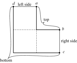
Figure 2. The quadrilateral $D_{1}$

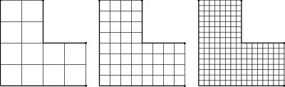
Figure 3. The first three subdivisions of $D_{1}$

We considered this example because we were interested in the squared rectangles corresponding to the optimal weight functions for the fat flow moduli of this sequence of quadrilaterals. Given a tiling $\mathcal{T}$ (or, more generally, a shingling) of a conformal quadrilateral $Q$, a weight function on $\mathcal{T}$ is a non-negative real-valued function $\rho$ on the set of tiles of $\mathcal{T}$. If $\rho$ is a weight function on $\mathcal{T}$ and $t$ is a tile of $\mathcal{T}$, then $\rho(t)$ is the weight of $t$. One can use a weight function to assign “lengths” to paths in $Q$ and “areas” to subsets of $Q$. The $\rho$-length of a path $\alpha$ in $Q$ is the sum of the weights of the tiles that the image of $\alpha$ intersects, and the $\rho$-area $A_{\rho}(W)$ of a subset $W$ of $Q$ is the sum of the squares of the weights of the tiles that intersect $W$. One then defines the $\rho$-height $H_{\rho}$ of $Q$ to be the minimum $\rho$-length of a path in $Q$ that joins the top and bottom of $Q$, and one defines the $\rho$-area $A_{\rho}$ of $Q$ to be $A_{\rho}(Q)$. The fat flow modulus of $Q$ with respect to $\rho$ is $H_{\rho}^{2}/A_{\rho}$. The optimal weight function is a weight function whose fat flow modulus is the supremum of the fat flow moduli of weight functions; it exists and is unique up to scaling. There is a squared rectangle corresponding to $Q$ whose squares correspond to the tiles of $\mathcal{T}$ with non-zero weights under the optimal weight function; furthermore, the side length of one of these squares is the weight of the corresponding tile.

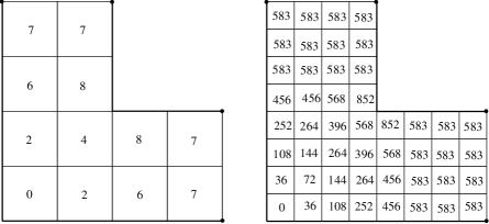
Figure 4. Optimal weight functions for the first two subdivisions of $D_{1}$

Figure 5. The squared rectangles and circle packings for the first three subdivisions of $D_{1}$

Figure 4 gives optimal weight functions for the first two subdivisions of the quadrilateral $D_{1}$, and the left side of Figure 5 gives the squared rectangles for the first three subdivisions of $D_{1}$. (See [1] for detailed information about optimal weight functions for tilings.) For each of these tilings of $D_{1}$, one can define a circle packing whose carrier complex is obtained from the tiling by adding a barycenter to each tile and then subdividing each tile into triangles by adding an edge from each vertex of the tile to the barycenter. By only drawing the edges of the packed carrier complex that correspond to edges of the tiling, one can use the circle packing to draw the tilings. On the right side of Figure 5, this is done for the first three subdivisions of $D_{1}$ using Stephenson’s program CirclePack [7].

While one cannot expect discrete functions from squared rectangles for tilings to converge to Riemann maps, He and Schramm showed in [5] that under general hypotheses discrete functions associated to circle packings converge to Riemann maps. It may seem that the squared rectangles and the circle packings are not closely related, but in some computational examples with the pentagonal and dodecahedral subdivision rules we have found that using our squared rectangle software [4] in conjuction with CirclePack [7] can lead to dramatic reductions in the total computation time for producing the packings. (In an example with over 1,600,000 vertices, using both programs led to a reduction in the computation time from almost 38 hours to under six hours.) We wondered whether the squared rectangles for the subdivisions of $D_{1}$ would define discrete functions which were closely related to the Riemann map for $D_{1}$.

But in this example the optimal weight functions appeared to be constant near the two sides of the quadrilateral. As we described above, if they really are constant then they couldn’t possibly give discrete approximations to the Riemann map. We found this “apparent” constancy of weights near the sides to be very surprising, and decided to look more closely at optimal weight functions for quadrilaterals made out of square tiles.

Example 2.2.

Let $D$ be the dumbbell drawn in Figure 1. The left edge of $D$ is the left side of the left ball, and the right edge of $D$ is the right side of the ride ball. The bar of $D$ has height $1$ and width $8$. Figure 6 gives squared rectangles for the first three subdivisions of $D$. For these subdivisions, the weights $p_{i}$ are constant on the entire bar and not just on the middle fourth of the bar.

Figure 6. Squared rectangles for the first three subdivisions of $D$

Example 2.3.

The dumbbell $D_{2}$ shown in Figure 7 is similar to the dumbbell $D$. The two dumbbells have the same bars, but for $D_{2}$ the left and right balls are smaller. The left edge of $D_{2}$ is the top side of the left ball and the right edge of $D_{2}$ is the top side of the right ball. Squared rectangles for the first three subdivisions of $D_{2}$ are shown in Figure 8. The dumbbell theorem guarantees that the weights are constant in the middle fourth of the bar, but here they are constant on most of the bar. The quadrilateral $D_{1}$ is a subcomplex of $D_{2}$.

Figure 7. The dumbbell $D_{2}$

Figure 8. Squared rectangles for the first three subdivisions of $D_{2}$

3. Weight vectors

This section deals with basic properties of vectors in Euclidean space.

We fix a positive integer $n$, which will be the bar height of a dumbbell under consideration. A weight vector is an element of $\mathbf{R}^{n}$ whose components are all nonnegative and not all 0. We denote by $\mathcal{W}$ the set of all weight vectors in $\mathbf{R}^{n}$. The height $H(x)$ and area $A(x)$ of a weight vector $x=(x_{1},\dotsc,x_{n})$ are defined by

$$H(x)=\sum_{i=1}^{n}x_{i}\quad\text{and}\quad A(x)=\sum_{i=1}^{n}x_{i}^{2}.$$

Given a positive real number $h$, we let $w_{h}={\textstyle(\frac{h}{n},\dotsc,\frac{h}{n})}$ and

$$\mathcal{W}_{h}=\{x\in\mathcal{W}:H(x)=h\}.$$

We see that $w_{h}\in\mathcal{W}_{h}$ and that $A(w_{h})=\frac{h^{2}}{n}$.

Lemma 3.1.

Let $h$ be a positive real number, let $x_{1},x_{2}\in\mathcal{W}_{h}$, and let $d_{1}$ and $d_{2}$ be the distances from $x_{1}$ and $x_{2}$ to $w_{h}$. Then $A(x_{1})\leq A(x_{2})$ if and only if $d_{1}\leq d_{2}$.

Proof.

Let $x\in\mathcal{W}_{h}$. Since $H(x)$ is the dot product of $x$ with the vector whose components are all 1, we have that $x\cdot(\frac{n}{h}w_{h})=h$. Hence $x\cdot w_{h}=\frac{h^{2}}{n}=w_{h}\cdot w_{h}$. So the square of the distance from $x$ to $w_{h}$ is

$$(x-w_{h})\cdot(x-w_{h})=x\cdot x-2x\cdot w_{h}+w_{h}\cdot w_{h}=x\cdot x-w_{h}\cdot w_{h}.$$

Thus decreasing $A(x)$ is equivalent to decreasing the distance from $x$ to $w_{h}$. This proves the lemma.

∎

Corollary 3.2.

The weight vector $w_{h}$ is the unique element of $\mathcal{W}_{h}$ with least area.

Lemma 3.3.

Let $x$ and $y$ be distinct weight vectors such that $A(x)\geq A(y)$. Then the area function restricted to the line segment from $x$ to $y$ is strictly decreasing at $x$.

Proof.

The line segment from $x$ to $y$ is traversed by $(y-x)t+x$ as the parameter $t$ varies from 0 to 1. We have that

$$A((y-x)t+x)=((y-x)t+x)\cdot((y-x)t+x)=(y-x)\cdot(y-x)t^{2}+2x\cdot(y-x)t+x\cdot x.$$

Viewing this as a function of $t$, its derivative at $t=0$ is $2x\cdot(y-x)$. But since

$$x\cdot x-2x\cdot y+y\cdot y=(x-y)\cdot(x-y)>0,$$

we have that $2x\cdot y<x\cdot x+y\cdot y$. So

$$2x\cdot(y-x)=2x\cdot y-2x\cdot x<y\cdot y-x\cdot x=A(y)-A(x)\leq 0.$$

This proves the lemma.

∎

Lemma 3.4.

Every nonempty compact convex set of weight vectors in $\mathbf{R}^{n}$ contains a unique weight vector with minimal area.

Proof.

Let $C$ be a nonempty compact convex set of weight vectors in $\mathbf{R}^{n}$. Since the area function is continuous, it has a minimum on $C$. Let $x$ and $y$ be weight vectors in $C$ with minimal area. Lemma 3.3 implies that if $x\neq y$, then the area function restricted to the line segment from $x$ to $y$ is decreasing at $x$. This is impossible because $x$ and $y$ have minimal area, and so $x=y$.

This proves Lemma 3.4.

∎

4. Weight functions which are sums of strictly monotonic cuts

This section deals with weight functions on rectangles that are viewed as conformal quadrilaterals. Eventually such a rectangle will be chosen to be contained in the bar of a dumbbell with the top of the rectangle in the top of the bar and the bottom of the rectangle in the bottom of the bar.

Let $R$ be a rectangle in the plane tiled in the straightforward way by squares with $n$ rows and $m$ columns of squares. Let $T_{ij}$ be the square in row $i$ and column $j$ for $i\in\{1,\ldots,n\}$ and $j\in\{1,\ldots,m\}$. With an eye toward combinatorial conformal moduli, we view $R$ as a quadrilateral in the straightforward way. A skinny cut for $R$ is strictly monotonic if it contains exactly one tile in every column of $R$. A weight function $\rho$ on $R$ is a sum of strictly monotonic skinny cuts if $\rho$ is a nonnegative linear combination of characteristic functions of strictly monotonic skinny cuts.

Lemma 4.1.

In the situation of the previous paragraph, the weight function $\rho$ is a sum of strictly monotonic skinny cuts if and only if for every $j\in\{1,\ldots,m-1\}$ we have that

$$\sum_{i=1}^{n}\rho(T_{ij})=\sum_{i=1}^{n}\rho(T_{i\,j+1})$$

and

$$\sum_{i=1}^{k}\rho(T_{ij})\leq\sum_{i=1}^{k+1}\rho(T_{i\,j+1})\text{ and }\sum_{i=1}^{k}\rho(T_{i\,j+1})\leq\sum_{i=1}^{k+1}\rho(T_{ij})\text{ for every }k\in\{1,\dotsc,n-1\}.$$

Proof.

Suppose that $\rho$ is a sum of strictly monotonic skinny cuts. Let $j\in\{1,\ldots,m-1\}$, and let $k\in\{1,\ldots,n-1\}$. Then every skinny cut defining $\rho$ which contains one of $T_{1j},\dotsc,T_{kj}$ also contains one of $T_{1\,j+1},\dotsc,T_{k+1\,j+1}$. Since $\rho$ is a nonnegative linear combination of such skinny cuts, it follows that

$$\sum_{i=1}^{k}\rho(T_{ij})\leq\sum_{i=1}^{k+1}\rho(T_{i\,j+1}).$$

Likewise

$$\sum_{i=1}^{k}\rho(T_{i\,j+1})\leq\sum_{i=1}^{k+1}\rho(T_{ij}).$$

In the case $k=n$, every skinny cut defining $\rho$ which contains one of $T_{1j},\dotsc,T_{nj}$ also contains one of $T_{1\,j+1},\dotsc,T_{n\,j+1}$. So

$$\sum_{i=1}^{n}\rho(T_{ij})\leq\sum_{i=1}^{n}\rho(T_{i\,j+1}).$$

The opposite inequality holds by symmetry, and so the inequality is actually equality. This proves the forward implication of the lemma.

For the backward implication, suppose that these equalities and inequalities are satisfied. We argue by induction on the number $N$ of tiles $T_{ij}$ such that $\rho(T_{ij})\neq 0$. The statement to be proved is vacuously true if $N=0$. So suppose that $N>0$ and that the statement is true for smaller values of $N$. Let $j\in\{1,\dotsc,m\}$. Since the zero function is not an allowable weight function and since column sums of $\rho$-weights are equal, it follows that the sum of the $\rho$-weights of the tiles in column $j$ is not 0. Let $S_{j}$ be the tile $T_{ij}$ with the smallest value of $i$ such that $\rho(T_{ij})\neq 0$. The inequalities imply that $\{S_{1},\dotsc,S_{m}\}$ is a strictly monotonic skinny cut. Let $c=\min\{\rho(S_{1}),\dotsc,\rho(S_{m})\}$. Let $\rho^{\prime}$ be the function on the tiles of $R$ gotten from $\rho$ by subtracting $c$ times the characteristic function of $\{S_{1},\dotsc,S_{m}\}$. If $\rho^{\prime}$ is the zero function, then $\rho$ is just $c$ times the characteristic function of $\{S_{1},\dotsc,S_{m}\}$. Otherwise $\rho^{\prime}$ is a weight function which satisfies the inequalities and it has value 0 at more tiles than does $\rho$. So by induction $\rho^{\prime}$ is a sum of strictly monotonic skinny cuts. It follows that $\rho$ is too.

This completes the proof of Lemma 4.1.

∎

Lemma 4.2.

Let $R$ be a rectangle as above tiled by $n$ rows and $m$ columns of squares $T_{ij}$. Let $x=(x_{1},\dotsc,x_{n})$ be a weight vector in $\mathbf{R}^{n}$. Then there exists a unique weight function $\rho$ for $R$ with minimal area subject to the conditions that $\rho$ is a sum of strictly monotonic skinny cuts and $\rho(T_{i1})=x_{i}$ for every $i\in\{1,\ldots,n\}$.

Proof.

If $\rho$ is a weight function for $R$ which is a sum of strictly monotonic skinny cuts such that $\rho(T_{i1})=x_{i}$ for $i\in\{1,\ldots,n\}$, then the $\rho$-height of $R$ is $H(x)$. Thus to minimize area, we may restrict to weight functions whose weights are all at most $H(x)$. Lemma 4.1 shows that we are minimizing area over a compact convex subset of $\mathbf{R}^{nm}$. This subset of $\mathbf{R}^{nm}$ is nonempty because it contains the weight vector corresponding to the weight function $\rho$ for $R$ for which $\rho(T_{ij})=x_{i}$ for every $i$ and $j$. Now Lemma 3.4 completes the proof of Lemma 4.2.

∎

5. The skinny cut function

We maintain the setting of Section 4, and continue to let $\mathcal{W}$ denote the set of all weight vectors in $\mathbf{R}^{n}$. Lemma 4.2 allows us to define a function $\Phi:\mathcal{W}\to\mathcal{W}$ as follows. Let $x=(x_{1},\dotsc,x_{n})\in\mathcal{W}$. We apply Lemma 4.2 in the case where $m=2$, so that the rectangle $R$ has $n$ rows and only two columns. Then there exists a unique weight function $\rho$ for $R$ with minimal area subject to the conditions that $\rho$ is a sum of strictly monotonic skinny cuts and $\rho(T_{i1})=x_{i}$ for $i\in\{1,\ldots,n\}$. Let $y=(y_{1},\dotsc,y_{n})$ be the weight vector such that $y_{i}=\rho(T_{i2})$ for $i\in\{1,\ldots,n\}$. We set $\Phi(x)=y$. This defines $\Phi$, which we call the skinny cut function. This section is devoted to the investigation of $\Phi$.

Let $x\in\mathcal{W}$, and let $h=H(x)$. Lemma 4.1 implies that $H(\Phi(x))=h$, so $\Phi$ maps $\mathcal{W}_{h}$ into $\mathcal{W}_{h}$. Moreover it is not difficult to see that if $r$ is a positive real number, then $\Phi(rx)=r\Phi(x)$.

Let $h$ be a positive real number, and let $x\in\mathcal{W}_{h}$. From $x$ we obtain real numbers $p_{0}=0\leq p_{1}\leq p_{2}\leq\cdots\leq p_{n}=h$ by setting $p_{k}=\sum_{i=1}^{k}x_{i}$ for $k\in\{0,\ldots,n\}$. We denote $(p_{0},\dotsc,p_{n})$ by $\pi(x)$ and we call it a weak partition of the closed interval $[0,h]$ as opposed to a strict partition in which the numbers $p_{0},\dotsc,p_{n}$ are required to be distinct. We call $p_{k}$ the $k$th partition point of $x$. This correspondence gives a bijection between $\mathcal{W}_{h}$ and the set of all weak partitions of $[0,h]$.

The inequalities of Lemma 4.1 can be easily interpreted in terms of partition points. Let $R$ be a rectangle as before with $n$ rows and two columns of tiles. Let $\rho$ be a weight function on $R$ which is a sum of strictly monotonic skinny cuts. Let $x=(x_{1},\dotsc,x_{n})$ and let $y=(y_{1},\dotsc,y_{n})$, where $x_{i}=\rho(T_{i1})$ and $y_{i}=\rho(T_{i2})$ for each $i$. Let $(p_{0},\dotsc,p_{n})=\pi(x)$, and let $(q_{0},\dotsc,q_{n})=\pi(y)$. Lemma 4.1 implies that $H(x)=H(y)$. Then, assuming that $H(x)=H(y)$, the inequalities of Lemma 4.1 are equivalent to the inequalities $q_{k-1}\leq p_{k}\leq q_{k+1}$ for every $k\in\{1,\ldots,n-1\}$. Likewise, assuming that $H(x)=H(y)$, the inequalities of Lemma 4.1 are equivalent to the inequalities $p_{k-1}\leq q_{k}\leq p_{k+1}$ for every $i\in\{1,\ldots,n-1\}$. We say that two weight vectors $x$ and $y$ are compatible if $H(x)=H(y)$ and $q_{k-1}\leq p_{k}\leq q_{k+1}$, equivalently $p_{k-1}\leq q_{k}\leq p_{k+1}$, for every $k\in\{1,\ldots,n-1\}$, where $(p_{0},\dotsc,p_{n})=\pi(x)$ and $(q_{0},\dotsc,q_{n})=\pi(y)$. This gives us the following reformulation of the definition of $\Phi$, formally stated as a lemma.

Lemma 5.1.

If $x$ is a weight vector, then $\Phi(x)$ is the weight vector with minimal area which is compatible with $x$.

Let $x=(x_{1},\dotsc,x_{n})\in\mathcal{W}$, and let $(p_{0},\dotsc,p_{n})=\pi(x)$. Let $k\in\{1,\ldots,n-1\}$. We call $p_{k}$ a left leaner for $x$ if $x_{k}>x_{k+1}$, and we call $p_{k}$ a right leaner for $x$ if $x_{k}<x_{k+1}$. The rest of this paragraph explains this terminology. Suppose that $p_{k}$ is a left leaner for $x$ for some $k\in\{1,\ldots,n-1\}$. Then $x_{k}>x_{k+1}$. The function $f(t)=(t-p_{k-1})^{2}+(p_{k+1}-t)^{2}$ is convex on the closed interval $[p_{k-1},p_{k+1}]$ with a minimum at the interval’s midpoint. This and the inequality $x_{k}>x_{k+1}$ imply that decreasing $p_{k}$ while fixing all other partition points of $x$ decreases the area of $x$. So we view $p_{k}$ as leaning left toward a position of less area for $x$. A similar discussion holds for right leaners.

Lemma 5.1 and the previous paragraph imply for every $x\in\mathcal{W}$ that $A(\Phi(x))<A(x)$ unless $x$ has no leaners. But if $x$ has no leaners, then $x=w_{h}$, where $h=H(x)$. Corollary 3.2 implies that $\Phi(w_{h})=w_{h}$. Thus for every positive real number $h$ the restriction of $\Phi$ to $\mathcal{W}_{h}$ has a unique fixed point, namely, $w_{h}$. We formally state some of the results just proved in the following lemma.

Lemma 5.2.

For every positive real number $h$ the restriction of $\Phi$ to $\mathcal{W}_{h}$ is a function $\Phi\big{|}_{\mathcal{W}_{h}}\colon\mathcal{W}_{h}\to\mathcal{W}_{h}$ which reduces areas of weight vectors except for at the unique fixed point, $w_{h}$.

Now let $x$ and $y$ be compatible weight vectors with $(p_{0},\dotsc,p_{n})=\pi(x)$ and $(q_{0},\dotsc,q_{n})=\pi(y)$. Suppose that $q_{k}$ is a left leaner for $y$ for some $k\in\{1,\ldots,n-1\}$. We say that $x$ blocks $q_{k}$ if $q_{k}=p_{k-1}$. The motivation behind this terminology is that for $x$ and $y$ to be compatible the inequality $q_{k}\geq p_{k-1}$ must be satisfied, and so even though $q_{k}$ is leaning left, $x$ prevents us from decreasing $q_{k}$ to decrease the area of $y$. Similarly, if $q_{k}$ is a right leaner for $y$, then we say that $x$ blocks $q_{k}$ if $q_{k}=p_{k+1}$.

Lemma 5.3.

Let $x$ and $y$ be compatible weight vectors. Then every left leaner for $y$ which is blocked by $x$ is a left leaner for $x$. Similarly, every right leaner for $y$ which is blocked by $x$ is a right leaner for $x$.

Proof.

Suppose that $x=(x_{1},\dotsc,x_{n})$, $y=(y_{1},\dotsc,y_{n})$, $\pi(x)=(p_{0},\dotsc,p_{n})$, and $\pi(y)=(q_{0},\dotsc,q_{n})$. Suppose that $q_{k}$ is a left leaner for $y$ blocked by $x$ for some $k\in\{1,\ldots,n-1\}$. This means that $y_{k}>y_{k+1}$ and that $q_{k}=p_{k-1}$. Since $q_{k-1}\geq p_{k-2}$, we have $y_{k}\leq x_{k-1}$. Since $q_{k+1}\geq p_{k}$, we have $y_{k+1}\geq x_{k}$. Combining these inequalities, we obtain that $x_{k-1}\geq y_{k}>y_{k+1}\geq x_{k}$, and so $p_{k-1}$ is a left leaner for $x$. Hence every left leaner for $y$ which is blocked by $x$ is a left leaner for $x$. A similar argument holds for right leaners.

This proves Lemma 5.3.

∎

Lemma 5.4.

Let $x\in\mathcal{W}$. Then every left leaner for $\Phi(x)$ is a left leaner for $x$ blocked by $x$, and every right leaner for $\Phi(x)$ is a right leaner for $x$ blocked by $x$. Conversely, if $y$ is a weight vector compatible with $x$ such that every leaner for $y$ is blocked by $x$, then $y=\Phi(x)$.

Proof.

Let $q$ be a left leaner for $\Phi(x)$. Then $q$ is blocked by $x$, for otherwise it is possible to decrease $A(\Phi(x))$ by decreasing $q$. Thus every left leaner for $\Phi(x)$ is blocked by $x$. Now Lemma 5.3 implies that every left leaner for $\Phi(x)$ is a left leaner for $x$. Similarly, every right leaner for $\Phi(x)$ is a right leaner for $x$ blocked by $x$.

Now suppose that $y$ is a weight vector compatible with $x$ such that every leaner for $y$ is blocked by $x$. Suppose that $y\neq\Phi(x)$. All weight vectors on the line segment from $y$ to $\Phi(x)$ are compatible with $x$. Lemma 3.3 implies that the area function restricted to this line segment is strictly decreasing at $y$. But as we move the partition points of $y$ linearly toward the partition points of $\Phi(x)$ we either move leaners away from blocked positions, which increases area, or we move nonleaners, which also increases area. Thus $y=\Phi(x)$.

This proves Lemma 5.4.

∎

We next introduce the notion of segments. Let $x\in\mathcal{W}_{h}$ for some positive real number $h$, and let $\pi(x)=(p_{0},\dotsc,p_{n})$. Let $i$ and $j$ be indices such that $p_{i}$ is either 0 or a leaner of $x$, $p_{j}$ is either $h$ or a leaner of $x$, $i<j$ and $p_{k}$ is not a leaner of $x$ if $i<k<j$. Then $x_{i+1}=\cdots=x_{j}$, $x_{i}\neq x_{i+1}$ if $i>0$, and $x_{j+1}\neq x_{j}$ if $j<n$. We call $(x_{i+1},\dotsc,x_{j})$ a segment of $x$. In other words, the leaners of $x$ parse $x$ into segments such that the coordinates of $x$ in every segment are equal, and segments are maximal with respect to this property. We call $p_{i}$ and $p_{j}$ the endpoints of the segment $(x_{i+1},\dotsc,x_{j})$. By the value of a segment we mean the value of any component of $x$ in that segment. By the dimension of a segment we mean the number of components in it. By the height of a segment we mean the sum of its components. Each endpoint of a segment is either a leaner or an endpoint of the interval $[0,h]$. If the left endpoint of a segment is a left leaner, then we say that it leans away from the segment, and if it is a right leaner, then we say that it leans toward the segment. The situation is similar for right endpoints.

Let $y$ be a weight vector in the image of $\Phi$. A weight vector $x$ is called a minimal preimage of $y$ if it satisfies the following:

1. $\Phi(x)=y$.

2. If $x^{\prime}$ is a weight vector with $\Phi(x^{\prime})=y$, then $A(x)\leq A(x^{\prime})$, with equality if and only if $x=x^{\prime}$.

Lemma 5.5.

Let $y$ be a weight vector, and let $t_{1},\dotsc,t_{m}$ be the segments of $y$ in order. Then $y$ is in the image of $\Phi$ if and only if there is a weight vector $x$ with segments $s_{1},\dotsc,s_{m}$ in order which satisfies the following:

1. The height of $s_{i}$ equals the height of $t_{i}$ for $i\in\{1,\ldots,m\}$.

2. For every $i\in\{1,\ldots,m\}$ the dimension of $s_{i}$ is the dimension of $t_{i}$ plus $\alpha_{i}-\tau_{i}$ where $\alpha_{i}$ is the number of endpoints of $t_{i}$ which lean away from $t_{i}$ and $\tau_{i}$ is the number of endpoints of $t_{i}$ which lean toward $t_{i}$.

Furthermore, if $y$ is in the image of $\Phi$ then this vector $x$ is unique and is the minimal preimage of $y$.

Proof.

We first suppose that $y$ is in the image of $\Phi$, and let $w$ be a weight vector such that $\Phi(w)=y$. Suppose that the right endpoint of $t_{1}$ leans toward $t_{1}$, namely, that it is a left leaner. Suppose that the right endpoint of $t_{1}$ is partition point $k$ of $y$. Lemma 5.4 implies that this left leaner is blocked by $w$, and so it is partition point number $k-1$ of $w$. This proves that if the right endpoint of $t_{1}$ leans toward $t_{1}$, then the dimension of $t_{1}$ is at least 2. Similarly, if the left endpoint of the last segment $t_{m}$ leans toward $t_{m}$, then the dimension of $t_{m}$ is at least 2. More generally, if both endpoints of some segment of $y$ lean toward that segment, then the dimension of that segment is at least 3. With the results of this paragraph and the fact that $\sum_{i=1}^{m}(\alpha_{i}-\tau_{i})=0$, we see that conditions 1 and 2 in the statement of Lemma 5.5 uniquely determine a weight vector $x$.

For the converse, suppose that $x$ is a weight vector with segments $s_{1},\dotsc,s_{m}$ in order which satisfies conditions 1 and 2 of the lemma. An induction argument on $i$ shows that the endpoints of $t_{i}$ other than 0 and $h$ are blocked by $x$ and that $x$ is compatible with $y$. By Lemma 5.4, $\Phi(x)=y$ and so $y$ is in the image of $\Phi$.

For the last statement, suppose that $y$ is in the image of $\Phi$. Let $x$ be the weight vector which satisfies conditions 1 and 2 of the lemma, and let $x^{\prime}$ be a weight vector with $\Phi(x^{\prime})=y$. Let $i\in\{1,\ldots,m\}$. Because the endpoints of $t_{i}$ other than 0 and $h$ are blocked by $x^{\prime}$, the number of components of $x^{\prime}$ between these endpoints equals the number of components of $x$ between these endpoints, namely, the dimension of $s_{i}$. But since the components of $s_{i}$ are all equal, Corollary 3.2 implies that the area of $s_{i}$ is at most the sum of the squares of the corresponding components of $x^{\prime}$. Thus $A(x)\leq A(x^{\prime})$, and equality holds if and only if $x=x^{\prime}$.

This proves Lemma 5.5. ∎

This section has thus far been concerned with the definition of $\Phi$ and basic relationships between a weight vector and its image under $\Phi$. We now turn to area estimates. The next result, Theorem 5.6, prepares for Theorem 5.7, which is the key ingredient in our proof of the dumbbell theorem.

Theorem 5.6.

Let $h$ be a positive real number, and let $x\in\mathcal{W}_{h}$. Then there exists a weight vector $w\in\mathcal{W}_{h}$ satisfying the following conditions.

1. Both $w$ and $\varPhi(w)$ have at most two segments with nonzero values. Furthermore, if they have two segments with nonzero values, then these segments are consecutive.

2. The weight vector $w$ is the minimal preimage of $\varPhi(w)$.

3. $A(w)\leq A(x)$.

4. $A(\varPhi(w))\geq A(\varPhi(x))$.

Proof.

Set

$$W=\{z\in\mathcal{W}_{h}:A(z)\leq A(x)\text{ and }A(\Phi(z))\geq A(\Phi(x))\}.$$

Since every element of $W$ satisfies conditions 3 and 4, it suffices to prove that $W$ contains a weight vector satisfying conditions 1 and 2. We will do this by first proving that $W$ contains an element with minimal area. It follows that $w$ is the minimal preimage of $\Phi(w)$, giving condition 2. We then prove that $w$ satisfies condition 1.

In this paragraph we prove that $W$ contains an element with minimal area. Since $x\in W$, $W$ is not empty. The set $\mathcal{W}_{h}$ is compact, and so the closure $\overline{W}$ of $W$ in $\mathcal{W}_{h}$ is compact. Since the area function is continuous, there exists a weight vector $w$ in $\overline{W}$ with minimal area. Because the area function is continuous and $w\in\overline{W}$, we have that $A(w)\leq A(x)$. It remains to prove that $A(\Phi(w))\geq A(\Phi(x))$. For this let $w^{\prime}$ be a weight vector in $W$ near $w$. Lemma 5.1 shows that $\Phi(w)$ is compatible with $w$. Because $w^{\prime}$ is near $w$, there exists a weight vector $y$ near $\Phi(w)$ which is compatible with $w^{\prime}$. Because $y$ is near $\Phi(w)$ the area of $y$ is not much larger than the area of $\Phi(w)$. Now Lemma 5.1 shows that the area of $\Phi(w^{\prime})$ is not much larger than the area of $\Phi(w)$. Since $A(\Phi(w^{\prime}))\geq A(\Phi(x))$, it follows that $A(\Phi(w))\geq A(\Phi(x))$. Thus $w\in W$. This proves that $W$ contains an element with minimal area.

We fix an element $w$ in $W$ with minimal area. Lemma 5.5 implies that $w$ is the minimal preimage of $\Phi(w)$. To prove Theorem 5.6 it suffices to prove that $w$ cannot have nonconsecutive segments with nonzero values. We do this by contradiction. So suppose that $w$ has nonconsecutive segments with nonzero values. Let $s_{1},\dotsc,s_{m}$ be the segments of $w$ in order with dimensions $d_{1},\dotsc,d_{m}$, values $v_{1},\dotsc,v_{m}$, and heights $h_{1},\dotsc,h_{m}$, so that $h_{i}=d_{i}v_{i}$ for every $i\in\{1,\ldots,m\}$.

In this paragraph we show that $w$ has two consecutive segments with nonzero values. We proceed by contradiction: suppose that $w$ does not have two consecutive segments with nonzero values. Then every other value of $w$ is $0$. Let $i\in\{1,\dotsc,m\}$ such that $v_{i}\neq 0$, $v_{i+1}=0$, and $v_{i+2}\neq 0$. Because of the symmetry with respect to the order of the components of $w$, we may, and do, assume that $v_{i}\leq v_{i+2}$. Let $A_{0}$ be the sum of the areas of the segments of $w$ other than $s_{i}$, $s_{i+1}$, and $s_{i+2}$. Then

$$A(w)=A_{0}+\frac{h_{i}^{2}}{d_{i}}+\frac{h_{i+2}^{2}}{d_{i+2}}.$$

Similarly, if $B_{0}$ is the sum of the areas of the segments of $\Phi(w)$ other than those corresponding to $s_{i}$, $s_{i+1}$, and $s_{i+2}$, then

$$A(\Phi(w))=B_{0}+\frac{h_{i}^{2}}{e_{i}}+\frac{h_{i+2}^{2}}{e_{i+2}},$$

where

$$e_{i}=\left\{\begin{array}[]{ll}d_{i}+1,&\hbox{if $i=1$}\\ d_{i}+2,&\hbox{if $i>1$}\\ \end{array}\right.$$

and

$$e_{i+2}=\left\{\begin{array}[]{ll}d_{i+2}+1,&\hbox{if $i=m$}\\ d_{i+2}+2,&\hbox{if $i<m$.}\\ \end{array}\right.$$

We construct a new weight vector $w^{\prime}$ by modifying $w$ as follows. Where $w$ has segments $s_{i}$, $s_{i+1}$, $s_{i+2}$ with heights $h_{i}$, $0$, $h_{i+2}$ and dimensions $d_{i}$, $d_{i+1}$, $d_{i+2}$, the weight vector $w^{\prime}$ has segments with heights $0$, $h_{i}$, $h_{i+2}$ and dimensions $d_{i}^{\prime}$, $d_{i}+1$, $d_{i+2}$. The heights and dimensions of all other segments of $w^{\prime}$ equal the corresponding heights and dimensions of $w$ except that if $i>1$, then $w^{\prime}$ has one fewer segment than $w$ because segment $s_{i-1}$ of $w$ has value $0$ and so the components of $w$ in $s_{i+1}$ must be adjoined to $s_{i-1}$. So

$$A(w^{\prime})=A_{0}+\frac{h_{i}^{2}}{d_{i}+1}+\frac{h_{i+2}^{2}}{d_{i+2}}<A(w)\leq A(x).$$

Using Lemma 5.5 we see that

$$A(\Phi(w^{\prime}))=B_{0}+\frac{h_{i}^{2}}{d_{i}+1}+\frac{h_{i+2}^{2}}{e_{i+2}}\geq A(\Phi(w))\geq A(\Phi(x)).$$

This contradicts the fact that $w$ is an element in $W$ with minimal area. Thus $w$ has two consecutive segments with nonzero values. If $w$ only has two segments with nonzero values, then we are done. Hence we may assume that $w$ has at least three segments with nonzero values.

Next suppose that $w^{\prime}$ is a weight vector with the same number of segments as $w$, the segments of $w^{\prime}$ have the same dimensions as the corresponding segments of $w$ but the leaners of $w^{\prime}$ are gotten by perturbing the leaners of $w$, equivalently, the heights of the segments of $w^{\prime}$ are gotten by perturbing the heights of the segments of $w$. If this perturbation is small enough, then Lemma 5.4 implies that $\Phi(w^{\prime})$ is gotten from $\Phi(w)$ by exactly the same perturbation. We will prove that there exists such a perturbation such that $A(w^{\prime})<A(w)$ and $A(\Phi(w^{\prime}))=A(\Phi(w))$. Thus $w^{\prime}$ is an element of $W$ with smaller area than $w$, a contradiction which will complete the proof of Theorem 5.6.

To begin the construction of such a perturbation, we note that the area of $w$ is

$$\sum_{i=1}^{m}d_{i}v_{i}^{2}=\sum_{i=1}^{m}d_{i}\left(\frac{h_{i}}{d_{i}}\right)^{2}=\sum_{i=1}^{m}\frac{1}{d_{i}}h_{i}^{2}=\sum_{i=1}^{m}a_{i}h_{i}^{2},$$

where $a_{i}=d_{i}^{-1}$ for every $i\in\{1,\ldots,m\}$. Recall that $w$ is the minimal preimage of $\varPhi(w)$. As above, if $t_{1},\dotsc,t_{m}$ are the segments of $\Phi(w)$ in order with dimensions $A_{1}^{-1},\dotsc,A_{m}^{-1}$, then the area of $\Phi(w)$ is

$$\sum_{i=1}^{m}A_{i}h_{i}^{2}.$$

This leads us to define functions $f\colon\mathbf{R}^{m}\to\mathbf{R}$ and $F\colon\mathbf{R}^{m}\to\mathbf{R}$ so that

$$f(x_{1},\dotsc,x_{m})=\sum_{i=1}^{m}a_{i}(x_{i}+h_{i})^{2}$$

and

$$F(x_{i},\dotsc,x_{m})=\sum_{i=1}^{m}A_{i}(x_{i}+h_{i})^{2}.$$

To prove Theorem 5.6, it suffices to find points $x=(x_{1},\dotsc,x_{m})\in\mathbf{R}^{m}$ arbitrarily near the origin 0 such that $\sum_{i=1}^{m}x_{i}=0$, $f(x)<f(0)$, $F(x)=F(0)$, and $x_{i}\geq 0$ if $h_{i}=0$.

We do this while fixing all but three components of $(x_{1},\dotsc,x_{m})$. We specify these components later in this paragraph. Since only three components of $(x_{1},\dotsc,x_{m})$ are allowed to vary, the functions $f$ and $F$ are really functions of three variables. To simplify notation, we now view $f$ and $F$ as functions from $\mathbf{R}^{3}$ to $\mathbf{R}$ with

$$f(x,y,z)=a(x+x_{0})^{2}+b(y+y_{0})^{2}+c(z+z_{0})^{2}+d$$

and

$$F(x,y,z)=A(x+x_{0})^{2}+B(y+y_{0})^{2}+C(z+z_{0})^{2}+D.$$

Since $w$ has two consecutive segments with nonzero values, by Lemma 5.5 $\Phi(w)$ has two consecutive segments with nonzero values. Let the variable $x$ correspond to a segment of $\Phi(w)$ with nonzero value which is adjacent to a segment with larger value. Let $z$ correspond to a segment of $\Phi(w)$ with maximal value. Let $y$ correspond to any segment of $\Phi(w)$ with nonzero value not already chosen. Note that $x_{0},y_{0},z_{0}>0$. Because the segment of $\Phi(w)$ corresponding to $x$ has an endpoint leaning away from it, its dimension $A^{-1}$ is at most as large as the dimension $a^{-1}$ of the corresponding segment of $w$. Thus $A^{-1}\leq a^{-1}$, and so $A\geq a$. Because the segment of $\Phi(w)$ corresponding to $z$ has no endpoint leaning away from it, $C^{-1}>c^{-1}$, and so $C<c$. Because the value of the segment of $\Phi(w)$ corresponding to $z$ is larger than the value of the segment corresponding to $x$, we have $Cz_{0}>Ax_{0}$. To prove Theorem 5.6 it suffices to find points $(x,y,z)\in\mathbf{R}^{3}$ arbitrarily near $(0,0,0)$ such that $x+y+z=0$, $f(x,y,z)<f(0,0,0)$, and $F(x,y,z)=F(0,0,0)$.

The set of all solutions $(x,y,z)$ to the equation $f(x,y,z)=f(0,0,0)$ is an ellipsoid containing the point $(0,0,0)$. The gradient of $f$ at $(0,0,0)$ is $(2ax_{0},2by_{0},2cz_{0})$. Because $ax_{0}$, $by_{0}$, $cz_{0}$ are not all equal, the plane given by $x+y+z=0$ contains the point $(0,0,0)$, but it is not tangent to the ellipsoid. Thus this plane intersects the ellipsoid in an ellipse. It likewise intersects the ellipsoid given by $F(x,y,z)=F(0,0,0)$ in an ellipse. These ellipses both lie in this plane and they have a point in common. If they intersect transversely at $(0,0,0)$, then it is easy to find points arbitrarily near $(0,0,0)$ which lie within the first ellipse and lie on the second one. In other words, Theorem 5.6 is true if the ellipses intersect transversely.

Finally, we assume that the ellipses are tangent at $(0,0,0)$. Let $L$ be the line in $\mathbf{R}^{3}$ tangent to the ellipses at $(0,0,0)$. Then $L$ lies in the plane given by $x+y+z=0$ and it lies in the tangent planes to both of the ellipsoids. These three planes have normal vectors given by $(1,1,1)$, $(ax_{0},by_{0},cz_{0})$ and $(Ax_{0},By_{0},Cz_{0})$. Thus these three vectors are linearly dependent. Thus the same is true for the columns of the matrix

$$\left[\begin{matrix}1&ax_{0}&Ax_{0}\\ 1&by_{0}&By_{0}\\ 1&cz_{0}&Cz_{0}\end{matrix}\right].$$

The cross product of any two rows is orthogonal to all three rows. The cross product of row 1 and row 3 is

$$v=((aC-Ac)x_{0}z_{0},Ax_{0}-Cz_{0},cz_{0}-ax_{0}).$$

Since $a\leq A$ and $C<c$, we have $(aC-Ac)x_{0}z_{0}<0$. Since $Cz_{0}>Ax_{0}$, we have $Ax_{0}-Cz_{0}<0$. Since $v$ is orthogonal to the rows of the preceding matrix, it is also orthogonal to the rows of

$$\left[\begin{matrix}\frac{1}{x_{0}}&a&A\\ \frac{1}{y_{0}}&b&B\\ \frac{1}{z_{0}}&c&C\end{matrix}\right].$$

So

$$(aC-Ac)x_{0}z_{0}\left(\frac{1}{x_{0}},\frac{1}{y_{0}},\frac{1}{z_{0}}\right)+(Ax_{0}-Cz_{0})(a,b,c)+(cz_{0}-ax_{0})(A,B,C)=(0,0,0).$$

Solving for $(a,b,c)$, we find that

$$(a,b,c)=r\left(\frac{1}{x_{0}},\frac{1}{y_{0}},\frac{1}{z_{0}}\right)+s(A,B,C)$$

for some real numbers $r$ and $s$ with $r<0$. Viewing $f(x,y,z)$ and $F(x,y,z)$ as dot products of vectors except for the final additive constants, we have that

$$f(x,y,z) -f(0,0,0)$$

$$=(a,b,c)\cdot((x+x_{0})^{2},(y+y_{0})^{2},(z+z_{0})^{2})-(a,b,c)\cdot(x_{0}^{2},y_{0}^{2},z_{0}^{2})$$

$$=(a,b,c)\cdot(x^{2}+2x_{0}x,y^{2}+2y_{0}y,z^{2}+2z_{0}z)$$

$$=r\left(\frac{1}{x_{0}},\frac{1}{y_{0}},\frac{1}{z_{0}}\right)\cdot(x^{2}+2x_{0}x,y^{2}+2y_{0}y,z^{2}+2z_{0}z)$$

$$\qquad+s(A,B,C)\cdot(x^{2}+2x_{0}x,y^{2}+2y_{0}y,z^{2}+2z_{0}z)$$

$$=r\left[\left(\frac{1}{x_{0}}x^{2}+\frac{1}{y_{0}}y^{2}+\frac{1}{z_{0}}z^{2}\right)+2(x+y+z)\right]+s[F(x,y,z)-F(0,0,0)]$$

$$=r\left(\frac{1}{x_{0}}x^{2}+\frac{1}{y_{0}}y^{2}+\frac{1}{z_{0}}z^{2}\right)+s[F(x,y,z)-F(0,0,0)].$$

So if $(x,y,z)$ is any point on the ellipse corresponding to $F$, then $F(x,y,z)-F(0,0,0)=0$ and so $f(x,y,z)-f(0,0,0)<0$, as desired.

This proves Theorem 5.6.

∎

Theorem 5.7.

Let $h$ be a positive real number. Let $x_{1},\dotsc,x_{3n}$ be weight vectors in $\mathcal{W}_{h}$ such that $A(x_{i+1})\leq A(\varPhi(x_{i}))$ for every $i\in\{1,\ldots,3n-1\}$. Then $x_{3n}=w_{h}$.

Proof.

Lemma 5.2 implies that $\varPhi$ does not increase area, and so

$$A(x_{1})\geq\cdots\geq A(x_{3n}).$$

Lemma 5.2 and Corollary 3.2 furthermore imply that if two of $x_{1},\dotsc,x_{3n}$ have the same area, then $x_{3n}=w_{h}$. So we may, and do, assume that $x_{1},\dotsc,x_{3n}$ are distinct.

Since $\varPhi(hx)=h\varPhi(x)$ for every weight vector $x\in\mathcal{W}_{1}$, we may, and do, assume that $h=1$.

Let $i\in\{1,\ldots,3n-1\}$. Theorem 5.6 implies that there exists a weight vector $x_{i}^{\prime}\in\mathcal{W}_{1}$ such that both $x^{\prime}_{i}$ and $\varPhi(x^{\prime}_{i})$ have at most two segments with nonzero values, the weight vector $x^{\prime}_{i}$ is the minimal preimage of $\varPhi(x^{\prime}_{i})$, $A(x^{\prime}_{i})\leq A(x_{i})$ and $A(\varPhi(x^{\prime}_{i}))\geq A(\varPhi(x_{i}))$. Set $x^{\prime}_{3n}=x_{3n}$. Then

$$A(x^{\prime}_{i+1})\leq A(x_{i+1})\leq A(\varPhi(x_{i}))\leq A(\varPhi(x^{\prime}_{i}))$$

for every $i\in\{1,\ldots,3n-1\}$. Thus to prove Theorem 5.7, we may replace $x_{1},\dotsc,x_{3n}$ by $x^{\prime}_{1},\dotsc,x^{\prime}_{3n}$. In other words we may, and do, assume for every $i\in\{1,\ldots,3n-1\}$ that $x_{i}$ and $\varPhi(x_{i})$ do not have nonconsecutive segments with nonzero values and that $x_{i}$ is the minimal preimage of $\varPhi(x_{i})$.

At this point the argument splits into two cases which depend on how many of the weight vectors $x_{1},\dotsc,x_{3n}$ have segments with value 0. In Case 1 we prove Theorem 5.7 under the assumption that at least $n$ of the weight vectors $x_{1},\dotsc,x_{3n}$ have a segment with value 0. In Case 2 we prove Theorem 5.7 under the assumption that fewer than $n$ of the weight vectors $x_{1},\dotsc,x_{3n}$ have a segment with value 0.

We begin Case 1 now. Assume that at least $n$ of the weight vectors $x_{1},\dotsc,x_{3n}$ have a segment with value 0. Let $z_{1},\dotsc,z_{n}$ be distinct elements of $\{x_{1},\dotsc,x_{3n}\}$ in order each of which has a segment with value 0. Then $A(z_{i+1})\leq A(\varPhi(z_{i}))$ for every $i\in\{1,\ldots,n-1\}$.

In this paragraph we show that in Case 1 it suffices to prove for every $i\in\{1,\ldots,n-1\}$ that

(5.8) $$A(z_{i+1})(A(z_{i})+1)-A(z_{i})\leq 0.$$

Indeed, this inequality is equivalent to the inequality

$$A(z_{i+1})\leq\frac{1}{A(z_{i})^{-1}+1}.$$

Since $H(z_{1})=1$, we have $A(z_{1})\leq 1$. A straightforward induction argument based on the preceding displayed inequality shows that $A(z_{i})\leq 1/i$ for every $i\in\{1,\ldots,n\}$. In particular $A(z_{n})\leq 1/n$. But Corollary 3.2 implies that $w_{1}$ is the unique element in $\mathcal{W}_{1}$ with area at most $1/n$. Hence $z_{n}=x_{3n}=w_{1}$. Thus to prove Theorem 5.7 in Case 1 it suffices to prove line 5.8 for every $i\in\{1,\ldots,n-1\}$.

In this paragraph we assume that there exists $i\in\{1,\ldots,n-1\}$ such that $z_{i}$ has only one segment with nonzero value. Let $d$ be the dimension of this segment. Then $A(z_{i})=1/d$. Moreover $\varPhi(z_{i})$ also has just one segment with nonzero value with dimension either $d+1$ or $d+2$. Hence $A(\varPhi(z_{i}))$ is either $1/(d+1)$ or $1/(d+2)$. So line 5.8 holds. Thus to prove Theorem 5.7 in Case 1 it suffices to prove line 5.8 under the assumption that $z_{i}$ has two segments with nonzero value.

So let $i\in\{1,\ldots,n-1\}$, and suppose that $z_{i}$ has two consecutive segments $s$ and $t$ in order with nonzero value. Let $p$ be the right endpoint of $s$, equivalently, the left endpoint of $t$. Let $d$ be the dimension of $s$, and let $e$ be the dimension of $t$. The value of $s$ is $p/d$, and the value of $t$ is $(1-p)/e$. It follows that

(5.9) $$A(z_{i})=d^{-1}p^{2}+e^{-1}(1-p)^{2}.$$

Let $d^{\prime}$ and $e^{\prime}$ be the dimensions of the segments $s^{\prime}$ and $t^{\prime}$ of $\varPhi(z_{i})$ corresponding to $s$ and $t$. Then

$$A(\varPhi(z_{i}))=(d^{\prime})^{-1}p^{2}+(e^{\prime})^{-1}(1-p)^{2}.$$

By symmetry we may assume that

$$\frac{p}{d^{\prime}}\leq\frac{1-p}{e^{\prime}}.$$

The last inequality implies that $p$ is a right leaner for $\varPhi(z_{i})$. Hence Lemma 5.4 implies that $p$ is a right leaner for $z_{i}$ and so

$$\frac{p}{d}\leq\frac{1-p}{e}.$$

Combining this with line 5.9 yields that

$$A(z_{i})=d^{-1}p^{2}+e^{-1}(1-p)^{2}\leq e^{-1}p(1-p)+e^{-1}(1-p)^{2}=e^{-1}(1-p).$$

Similarly, we have that

(5.10) $$A(\varPhi(z_{i}))\leq(e^{\prime})^{-1}(1-p).$$

Because $z_{i}$ has a segment with value 0 and $z_{i}$ is the minimal preimage of $\varPhi(z_{i})$, it is also true that $\varPhi(z_{i})$ has a segment with value 0. These facts and Lemma 5.5 imply that if $\varPhi(z_{i})$ has a segment with value 0 preceding $s^{\prime}$, then $d^{\prime}=d$ and $e^{\prime}\geq e+1$. If $\varPhi(z_{i})$ does not have a segment with value 0 preceding $s^{\prime}$, then $d^{\prime}=d-1$ and $e^{\prime}=e+2$.

Suppose that $\varPhi(z_{i})$ has a segment with value 0 preceding $s^{\prime}$. The previous paragraph shows that $d^{\prime}=d$ and $e^{\prime}\geq e+1$. Combining this with line 5.10 yields that $A(\varPhi(z_{i}))\leq(e+1)^{-1}(1-p)$. Hence

$$A(z_{i+1}) (A(z_{i})+1)-A(z_{i})$$

$$\leq A(\varPhi(z_{i}))(A(z_{i})+1)-A(z_{i})$$

$$\leq A(\varPhi(z_{i}))A(z_{i})+A(\varPhi(z_{i}))-A(z_{i})$$

$$\leq\frac{1}{e(e+1)}(1-p)^{2}+\frac{1}{d^{\prime}}p^{2}+\frac{1}{e^{\prime}}(1-p)^{2}-\frac{1}{d}p^{2}-\frac{1}{e}(1-p)^{2}$$

$$\leq\frac{1}{e(e+1)}(1-p)^{2}+\frac{1}{d}p^{2}+\frac{1}{e+1}(1-p)^{2}-\frac{1}{d}p^{2}-\frac{1}{e}(1-p)^{2}$$

$$\leq\frac{1}{e(e+1)}(1-p)^{2}-\frac{1}{e(e+1)}(1-p)^{2}$$

$$\leq 0.$$

Thus line 5.8 is true if $\varPhi(z_{i})$ has a segment with value 0 preceding $s^{\prime}$.

Next assume that $\varPhi(z_{i})$ does not have a segment with value 0 preceding $s^{\prime}$. Then the next-to-last paragraph shows that $d^{\prime}=d-1$ and $e^{\prime}=e+2$. Combining this with line 5.10 yields that $A(\varPhi(z_{i}))\leq(e+2)^{-1}(1-p)$. We also have that

$$\frac{p}{d-1}=\frac{p}{d^{\prime}}\leq\frac{1-p}{e^{\prime}}=\frac{1-p}{e+2}.$$

Hence

$$A(z_{i+1}) (A(z_{i})+1)-A(z_{i})$$

$$\leq A(\varPhi(z_{i}))(A(z_{i})+1)-A(z_{i})$$

$$\leq A(\varPhi(z_{i}))A(z_{i})+A(\varPhi(z_{i}))-A(z_{i})$$

$$\leq\frac{1}{e(e+2)}(1-p)^{2}+\frac{1}{d^{\prime}}p^{2}+\frac{1}{e^{\prime}}(1-p)^{2}-\frac{1}{d}p^{2}-\frac{1}{e}(1-p)^{2}$$

$$\leq\frac{1}{e(e+2)}(1-p)^{2}+\frac{1}{d-1}p^{2}+\frac{1}{e+2}(1-p)^{2}-\frac{1}{d}p^{2}-\frac{1}{e}(1-p)^{2}$$

$$\leq\frac{1}{e(e+2)}(1-p)^{2}+\frac{1}{(d-1)d}p^{2}-\frac{2}{e(e+2)}(1-p)^{2}$$

$$\leq\frac{1}{e(e+2)}(1-p)^{2}+\frac{1}{e(e+2)}(1-p)^{2}-\frac{2}{e(e+2)}(1-p)^{2}$$

$$\leq 0.$$

Thus line 5.8 is true if $\varPhi(z_{i})$ does not have a segment with value 0 preceding $s^{\prime}$.

The proof of Theorem 5.7 is now complete in Case 1, namely, Theorem 5.7 is proved if at least $n$ of the weight vectors $x_{1},\dotsc,x_{3n}$ have a segment with value 0.

Now we proceed to Case 2. Suppose that fewer than $n$ of the weight vectors $x_{1},\dotsc,x_{3n}$ have a segment with value 0. Then at least $2n$ of the weight vectors $x_{1},\dotsc,x_{3n}$ do not have a segment with value 0. Let $z_{1},\dotsc,z_{2n}$ be distinct elements of $\{x_{1},\dotsc,x_{3n}\}$ in order none of which has a segment with value 0. Then $A(z_{i+1})\leq A(\varPhi(z_{i}))$ for every $i\in\{1,\ldots,2n-1\}$. As we have seen, to finish the proof of Theorem 5.7, it suffices to prove that $z_{2n}=w_{1}$. We do this by contradiction. Suppose that $z_{2n}\neq w_{1}$. As we have seen, it follows that $z_{i}\neq w_{1}$ for $i\in\{1,\ldots,2n\}$.

Let $i\in\{1,\ldots,2n-1\}$. Then $z_{i}$ has at most two segments, $z_{i}$ has no segment with value 0, and $z_{i}$ is the minimal preimage of $\varPhi(z_{i})$. The only weight vector in $\mathcal{W}_{1}$ with one segment is $w_{1}$, so $z_{i}$ has two segments neither of which has value 0.

Let the first segment of $z_{i}$ have right endpoint $p$ and dimension $d$. Then the second segment of $z_{i}$ has left endpoint $p$ and dimension $n-d$. So

$$A(z_{i}) =\frac{1}{d}p^{2}+\frac{1}{(n-d)}(1-p)^{2}=\frac{(n-d)p^{2}+d(1-p)^{2}}{d(n-d)}$$

$$=\frac{np^{2}-dp^{2}+d-2dp+dp^{2}}{d(n-d)}=\frac{n^{2}p^{2}-2dnp+dn}{d(n-d)n}$$

$$=\frac{(np-d)^{2}-d^{2}+dn}{d(n-d)n}=\frac{(d-np)^{2}}{d(n-d)n}+\frac{1}{n}.$$

Set

$$B(z_{i})=\frac{(d-np)^{2}}{d(n-d)}.$$

Then

$$A(z_{i})=\frac{1}{n}B(z_{i})+\frac{1}{n}.$$

Since $z_{i}$ has two segments neither of which has value 0, the same is true of $\varPhi(z_{i})$. We define $B(\varPhi(z_{i}))$ in the same way that we define $B(z_{i})$. Then the given inequality $A(z_{i+1})\leq A(\varPhi(z_{i}))$ is equivalent to the inequality $B(z_{i+1})\leq B(\varPhi(z_{i}))$. We focus on this latter inequality.

Let $a$ be the positive real number such that $B(z_{i})=a^{2}$. Then

$$\begin{gathered}\frac{(d-np)^{2}}{d(n-d)}=a^{2}\\ (d-np)^{2}=a^{2}d(n-d)\\ d^{2}-nd+a^{-2}(d-np)^{2}=0\\ (d-\frac{n}{2})^{2}+a^{-2}(d-np)^{2}=\frac{n^{2}}{4}\\ \left(\frac{2d}{n}-1\right)^{2}+a^{-2}\left(\frac{2d}{n}-2p\right)^{2}=1.\end{gathered}$$

We are led to consider the family $\mathcal{E}$ of all ellipses of the form $x^{2}+a^{-2}y^{2}=1$, where $a$ is a positive real number. The open upper halves of the ellipses in $\mathcal{E}$ fill the open half infinite strip $S=\{(x,y)\in\mathbf{R}^{2}:|x|<1,y>0\}$.

The weight vector $z_{i}$ determines the point

$$P(z_{i})=(x_{i},y_{i})=\left(\frac{2d}{n}-1,\frac{2d}{n}-2p\right)$$

in $\mathbf{R}^{2}$, and we next show that we may assume that $P(z_{i})\in S$. It is easy to see that $|x_{i}|<1$, so what is needed is the inequality $y_{i}>0$. Since $z_{i}$ and $\varPhi(z_{i})$ have exactly one leaner, by symmetry we may, and do, assume that this leaner is a right leaner. Hence

$$\begin{gathered}\frac{1}{d}p<\frac{1}{n-d}(1-p)\\ p(n-d)<d(1-p)\\ pn<d.\end{gathered}$$

It follows that $y_{i}>0$, and so $P(z_{i})\in S$. It is even true that $y_{i}<x_{i}+1$, and so $P(z_{i})$ lies in the triangle $T=\{(x,y)\in\mathbf{R}^{2}:|x|<1,0<y<x+1\}$.

The point of $\mathbf{R}^{2}$ corresponding to $\varPhi(z_{i})$ likewise lies in $T$. Moreover since the first segment of $z_{i}$ has right endpoint $p$ and dimension $d$, it follows that the first segment of $\varPhi(z_{i})$ has right endpoint $p$ and dimension $d-1$. In other words, the point of $T$ corresponding to $\varPhi(z_{i})$ is

$$\left(\frac{2(d-1)}{n}-1,\frac{2(d-1)}{n}-2p\right)=\left(x_{i}-\frac{2}{n},y_{i}-\frac{2}{n}\right).$$

Now we can reformulate our problem as follows. Let $\tau\colon\mathbf{R}^{2}\to\mathbf{R}^{2}$ be the translation defined by $\tau(x,y)=\left(x-\frac{2}{n},y-\frac{2}{n}\right)$. We begin with a point $t_{1}\in T$. Let $E_{1}$ be the ellipse in $\mathcal{E}$ containing $t_{1}$. We have that $\tau(t_{1})\in T$ and $\tau(t_{1})$ lies within $E_{1}$. Let $E^{\prime}_{1}$ be the ellipse in $\mathcal{E}$ containing $\tau(t_{1})$. Let $t_{2}$ be a point of $T$ either on or within $E^{\prime}_{1}$. We iterate this construction to obtain points $t_{1},\dotsc,t_{2n}\in T$. To complete the proof of Theorem 5.7 it suffices to prove that it is impossible to construct points $t_{1},\dotsc,t_{2n}$ in this way.

To this end, let $A$ be the subset of $\mathbf{R}^{2}$ which is the union of the closed line segment joining $(0,0)$ with $(0,1)$ and the closed line segment joining $(0,1)$ with $(1,2)$. See Figure 9. We define a function $\alpha\colon T\to\mathbf{R}$ as follows. Let $t\in T$. There exists a unique ellipse $E\in\mathcal{E}$ which contains $t$, and $A\cap E$ consists of a single point. Let $\alpha(t)$ be the $y$-coordinate of this point.

Figure 9. Defining $\alpha(t)$.

We will prove that if $t_{1},\dotsc,t_{2n}$ are points in $T$ as in the next-to-last paragraph, then $\alpha(t_{i+1})<\alpha(t_{i})-1/n$ for every $i\in\{1,\ldots,2n-1\}$. This suffices to complete the proof of Theorem 5.7. Because $t_{i+1}$ lies either on or within the ellipse in $\mathcal{E}$ containing $\tau(t_{i})$, it actually suffices to prove that $\alpha(\tau(t_{i}))<\alpha(t_{i})-1/n$ for every $i\in\{1,\ldots,2n-1\}$, which is what we do.

So let $i\in\{1,\ldots,2n-1\}$. Let $E_{i}$ and $E^{\prime}_{i}$ be the ellipses in $\mathcal{E}$ which contain $t_{i}$ and $\tau(t_{i})$.

First suppose that the $x$-coordinates of both $t_{i}$ and $\tau(t_{i})$ are nonnegative. See Figure 10. In this case it is clear that we actually have that $\alpha(\tau(t_{i}))<\alpha(t_{i})-2/n$, as desired.

Figure 10. When the $x$-coordinates of both $t_{i}$ and $\tau(t_{i})$ are nonnegative.

Next suppose that the $x$-coordinates of both $t_{i}$ and $\tau(t_{i})$ are nonpositive. See Figure 11.

Figure 11. When the $x$-coordinates of both $t_{i}$ and $\tau(t_{i})$ are nonpositive.

Since $x^{2}+a^{-2}y^{2}=1$, we have that $y^{2}=a^{2}(1-x^{2})$. Differentiating this with respect to $x$ yields that $2yy^{\prime}=-2a^{2}x$. Solving for $y^{\prime}$ and replacing $a^{2}$ with $y^{2}/(1-x^{2})$ yields that

(5.11) $$y^{\prime}=\frac{xy}{x^{2}-1}.$$

Since $y<x+1$ and $x/(x^{2}-1)\geq 0$ if $-1<x\leq 0$, we have that $y^{\prime}<x/(x-1)$. It follows that $y^{\prime}<1/2$ throughout $T$. This implies that the vertical distance from $t_{i}$ to $E^{\prime}_{i}$ is at least $1/n$. Line 5.11 implies that $E_{i}$ increases more than $E^{\prime}_{i}$ as they approach $A$ from the left. It follows that $\alpha(\tau(t_{i}))<\alpha(t_{i})-1/n$, as desired.

Finally, if the $x$-coordinate of $t_{i}$ is positive and the $x$-coordinate of $\tau(t_{i})$ is negative, then an argument similar to that in the previous paragraph shows again that $\alpha(\tau(t_{i}))<\alpha(t_{i})-1/n$.

This completes the proof of Theorem 5.7.

∎

6. The proof of the dumbbell theorem

We prove the dumbbell theorem in this section.

Let $D$ be a dumbbell. Let $\rho$ be a fat flow optimal weight function for $D$. Let $h=H_{\rho}$. We scale $\rho$ so that it is a sum of minimal skinny cuts, making $h$ an integer. Suppose that $D$ has bar height $n$. Let $C_{1},\dotsc,C_{3n}$ be the leftmost $3n$ columns in $B$ in left-to-right order, and let $D_{1},\dotsc,D_{3n}$ be the rightmost $3n$ columns in $B$ in right-to-left order.

For every $i\in\{1,\ldots,3n\}$, applying $\rho$ to the tiles in $C_{i}$ obtains a weight vector $y_{i}\in\mathbf{R}^{n}$ and applying $\rho$ to the tiles in $D_{i}$ obtains a weight vector $z_{i}\in\mathbf{R}^{n}$. From the assumption that $H_{\rho}=h$, it follows that $H(y_{1})\geq h$, and so by scaling $y_{1}$ we can obtain a weight vector $x_{1}\in\mathcal{W}_{h}$ such that $A(x_{1})\leq A(y_{1})$. Let $j$ be the largest element of $\{1,\dotsc,3n\}$ such that there exist weight vectors $x_{1},\dotsc,x_{j}\in\mathcal{W}_{h}$ with $A(x_{1})\leq A(y_{1})$ and if $j>1$, then $A(x_{j})\geq A(y_{j})$ and $A(x_{i+1})\leq A(\varPhi(x_{i}))$ for every $i\in\{1,\ldots,j-1\}$. Similarly, let $k$ be the largest element of $\{1,\dotsc,3n\}$ such that there exist weight vectors $x_{1},\dotsc,x_{k}\in\mathcal{W}_{h}$ with $A(x_{1})\leq A(z_{1})$ and if $k>1$, then $A(x_{k})\geq A(z_{k})$ and $A(x_{i+1})\leq A(\varPhi(x_{i}))$ for every $i\in\{1,\ldots,k-1\}$.

In this paragraph we define a new weight function $\sigma$ on $D$. Let $t$ be a tile of $D$. If $t$ is contained in either one of the balls of $D$ or one of the columns $C_{1},\dotsc,C_{j-1},D_{k-1},\dotsc,D_{1}$, then $\sigma(t)=\rho(t)$. If $t$ is in $B$ and strictly between $C_{3n}$ and $D_{3n}$, then $\sigma(t)=h/n$. Now suppose that $t$ is contained in $C_{j}$. We have that $\rho$ is a sum of $h$ minimal skinny cuts. We define $\sigma(t)$ to be the number of these skinny cuts $c$ with the property that as $c$ proceeds from the left side of $D$ to $C_{j}$, the tile $t$ is the first tile of $C_{j}$ in $c$. This defines $\sigma(t)$ for every tile $t$ in $C_{j}$. These values determine a weight vector $\overline{x}_{j}\in\mathcal{W}_{h}$ in the straightforward way. If $j<3n$, then we use the weight vector $x_{j+1}=\varPhi(\overline{x}_{j})$ in the straightforward way to define $\sigma(t)$ for every tile $t$ in $C_{j+1}$. We inductively set $x_{i+1}=\varPhi(x_{i})$ and use this weight vector in the straightforward way to define $\sigma(t)$ for every tile $t$ in $C_{i+1}$ for every $i\in\{j+1,\ldots,3n-1\}$. This defines $\sigma(t)$ for every tile $t$ in $C_{j},\dotsc,C_{3n}$. We define $\sigma(t)$ for every tile $t$ in $D_{k},\dotsc,D_{3n}$ analogously. The definition of $\sigma$ is now complete.

By assumption there exist weight vectors $x_{1},\dotsc,x_{j}\in\mathcal{W}_{h}$ with $A(x_{1})\leq A(y_{1})$ and if $j>1$, then $A(x_{j})\geq A(y_{j})$ and $A(x_{i+1})\leq A(\varPhi(x_{i}))$ for every $i\in\{1,\ldots,j-1\}$. In defining $\sigma$ we constructed weight vectors $\overline{x}_{j},x_{j+1},\dotsc,x_{3n}\in\mathcal{W}_{h}$ with $x_{j+1}=\varPhi(\overline{x}_{j})$ and $x_{i+1}=\varPhi(x_{i})$ for every $i\in\{j+1,\ldots,3n-1\}$. We redefine $x_{j}$ to be $\overline{x}_{j}$. Then $x_{1},\dotsc,x_{3n}$ are weight vectors in $\mathcal{W}_{h}$ such that $A(x_{i+1})\leq A(\varPhi(x_{i}))$ for every $i\in\{1,\ldots,3n-1\}$. Theorem 5.7 implies that $x_{3n}=w_{h}$. The situation is analogous at the right end of $B$.

In this paragraph we prove that $H_{\sigma}=h$. Because $\sigma$ is constant on the union of the columns of $B$ between $C_{3n-1}$ and $D_{3n-1}$, the restriction of $\sigma$ to these columns is a sum of skinny cuts. The definition of $\varPhi$ implies that these skinny cuts can be extended to the columns of $B$ from $C_{j}$ to $D_{k}$ so that the restriction of $\sigma$ to the columns from $C_{j}$ to $D_{k}$ is a sum of skinny cuts. The definition of $\sigma$ implies that these skinny cuts can be extended to all of $D$ so that $\sigma$ is greater than or equal to a weight function which is a sum of $h$ skinny cuts. We conclude that $H_{\sigma}\geq h$. But since the columns of $D$ from $C_{j}$ to $D_{k}$ have $\sigma$-height $h$, it is in fact the case that $H_{\sigma}=h$.

In this paragraph we prove that $A_{\sigma}=A_{\rho}$. We proceed by contradiction. Suppose that $A_{\sigma}\neq A_{\rho}$. Since $H_{\sigma}=h=H_{\rho}$ and $\rho$ is optimal, it follows that $A_{\rho}<A_{\sigma}$. By definition $\rho$ and $\sigma$ agree away from the columns of $B$ from $C_{j}$ to $D_{k}$. Hence the values of $\rho$ on the tiles of one of the columns $C$ from $C_{j}$ to $D_{k}$ determines a weight vector in $\mathcal{W}_{h^{\prime}}$ for some $h^{\prime}\geq h$ whose area is less than the weight vector in $\mathcal{W}_{h}$ gotten from the values of $\sigma$ on the tiles of $C$. If $C$ is between $C_{3n}$ and $D_{3n}$, then the weight vector determined by $\sigma$ is $w_{h}$. Corollary 3.2 shows that this is impossible because the area of $w_{h}$ is minimal. Thus $C$ is either one of the columns $C_{j},\dotsc,C_{3n}$ or $D_{k},\dotsc,D_{3n}$. By symmetry we may assume that $C=C_{i}$ for some $i\in\{j,\ldots,3n\}$. Then $A(y_{i})<A(x_{i})$. By construction we have that $A(\overline{x}_{j})\leq A(y_{j})$. Since we replaced the original value of $x_{j}$ by $\overline{x}_{j}$, we have that $A(x_{j})\leq A(y_{j})$, and so $i>j$. Now we have a contradiction to the choice of $j$. This proves that $A_{\sigma}=A_{\rho}$.

Now we have that $H_{\sigma}=H_{\rho}$ and $A_{\sigma}=A_{\rho}$. It follows that $\sigma=\rho$. Since $\sigma$ is virtually bar uniform, we see that $\rho$ is virtually bar uniform.

This proves the dumbbell theorem.

7. Notes

In this section we state without proof a number of results related to the dumbbell theorem.

We say that a dumbbell $D$ is vertically convex if whenever $x$ and $y$ are points in $D$ such that the line segment joining them is vertical, then this line segment lies in $D$. We say that the sides of $D$ are extreme if the sides of $D$ are contained in vertical lines such that $D$ lies between these lines. Suppose that the vertical lines determined by our tiling of the plane intersect the $x$-axis in exactly the set of integers. We say that a skinny cut for $D$ is monotonic if it has an underlying path which is the graph of a function and that the restriction of this function to the interval determined by any pair of consecutive integers is either monotonically increasing or decreasing. If the dumbbell $D$ is vertically convex and its sides are extreme, then every optimal weight function for $D$ is a sum of monotonic minimal skinny cuts.

We recall Lemma 4.2. Let $R$ be a rectangle tiled by $n$ rows and $m$ columns of squares $T_{ij}$. Let $x=(x_{11},\dotsc,x_{n1})$ be a weight vector in $\mathbf{R}^{n}$. Then there exists a unique weight function $\rho$ for $R$ with minimal area subject to the conditions that $\rho$ is a sum of strictly monotonic skinny cuts and $\rho(T_{i1})=x_{i}$ for every $i\in\{1,\ldots,n\}$. The skinny cut function $\varPhi$ is defined so that if $m=2$, then $\varPhi(x)=(\rho(T_{12}),\dotsc,\rho(T_{n2}))$. It is in fact true for every $m\geq 2$ that $\varPhi^{j-1}(x)=(\rho(T_{1j}),\dotsc,\rho(T_{nj}))$ for every $j\in\{2,\ldots,m\}$.

Let $h$ be a positive real number, and let $x\in\mathcal{W}_{h}$. Let $\pi(x)=(p_{0},\dotsc,p_{n})$. We define a nonnegative integer $\mu_{i}$ for every $i\in\{1,\ldots,n-1\}$. Let $i\in\{1,\ldots,n-1\}$. If $p_{i}<\frac{hi}{n}$, then $\mu_{i}$ is the number of partition points $p_{i},\dotsc,p_{n-1}$ in the half-closed half-open interval $[p_{i},\frac{hi}{n})$. If $p_{i}>\frac{hi}{n}$, then $\mu_{i}$ is the number of partition points $p_{1},\dotsc,p_{i}$ in the half-open half-closed interval $(\frac{hi}{n},p_{i}]$. If $p_{i}=\frac{hi}{n}$, then $\mu_{i}=0$. Set $\mu=\max\{\mu_{1},\dotsc,\mu_{n-1}\}$. Note that $\mu\leq n-1$, and that $\mu=n-1$ for the weight vector $(0,0,0,\dotsc,h)$. It turns out that $\varPhi^{m}(x)=w_{h}$ for some nonnegative integer $m$ if and only if $m\geq\mu$. This implies that $\varPhi^{n-1}(x)=w_{h}$ for every weight vector $x\in\mathcal{W}_{h}$. In other words, if $x_{1},\dotsc,x_{n-1}$ are weight vectors in $\mathcal{W}_{h}$ such that $x_{i+1}=\varPhi(x_{i})$ for every $i\in\{1,\ldots,n-2\}$, then $x_{n-1}=w_{h}$. Compare this with Theorem 5.7. We see that the integer $3n$ in Theorem 5.7 cannot be replaced by an integer less than $n-1$. It is in fact true that there exists a positive real number $\epsilon$ such that the integer $3n$ in Theorem 5.7 cannot be replaced by an integer less than $(1+\epsilon)n$. It is probably true that $3n$ can be replaced by $3n/2$.

Not surprisingly, the skinny cut function $\varPhi$ is continuous. What might be surprising is that it is in fact piecewise affine. If $c_{n}$ denotes the number of affine pieces of $\varPhi$, then the sequence $(c_{n})$ satisfies a quadratic linear recursion with eigenvalue $1+\sqrt{2}$.

There exists a theory of combinatorial moduli “with boundary conditions”, as alluded to by Lemma 4.2. For simplicity we deal with a rectangle $R$ with $n$ rows of tiles. Let $h$ be a positive real number, and let $x$ be a weight vector in $\mathbf{R}^{n}$ with height $h$. Here are two ways to define optimal weight functions with boundary conditions. In the first way we minimize area over all weight functions on $R$ with fat flow height $h$ such that the values of $\rho$ on the first column of $R$ give $x$. In the second way we maximize the fat flow modulus over all weight functions on $R$ whose values on the first column of $R$ give a scalar multiple of $x$. It turns out that these constructions are equivalent. They yield a weight function which is unique up to scaling. Interpreted properly, most of the results of [1] hold in this setting. For example, the optimal weight function is a sum of minimal fat flows (modulo the first column). A straightforward modification of the algorithm for computing optimal weight functions even applies in this setting.

References

- [1] J. W. Cannon, W. J. Floyd, and W. R. Parry, Squaring rectangles: the finite Riemann mapping theorem, The mathematical legacy of Wilhelm Magnus: groups, geometry and special functions (Brooklyn, NY, 1992), Amer. Math. Soc., Providence, RI, 1994, pp. 133-212.
- [2] J. W. Cannon, W. J. Floyd, and W. R. Parry, Finite subdivision rules, Conform. Geom. Dyn. 5 (2001), 153–196 (electronic).
- [3] J. W. Cannon, W. J. Floyd, and W. R. Parry, Expansion complexes for finite subdivision rules I, Conform. Geom. Dyn. 10 (2006), 63–99 (electronic).
-
[4]
J. W. Cannon, W. J. Floyd, and W. R. Parry, precp.p,
software, available from
http://www.math.vt.edu/people/floyd. - [5] Z.-x. He and O. Schramm, On the convergence of circle packings to the Riemann map, Invent. math. 125 (1996), 285–305.
- [6] O. Schramm, Square tilings with prescribed combinatorics, Israel J. Math. 84 (1993), 97–118.
- [7] K. Stephenson, CirclePack, software, available from http://www.math.utk.edu/~kens.