Dislocations in graphene

Abstract

We study the stability and evolution of various elastic defects in a flat graphene sheet and the electronic properties of the most stable configurations. Two types of dislocations are found to be stable: “glide” dislocations consisting of heptagon-pentagon pairs, and “shuffle” dislocations, an octagon with a dangling bond. Unlike the most studied case of carbon nanotubes, Stone Wales defects are unstable in the planar graphene sheet. Similar defects in which one of the pentagon-heptagon pairs is displaced vertically with respect to the other one are found to be dynamically stable. Shuffle dislocations will give rise to local magnetic moments that can provide an alternative route to magnetism in graphene.

I Introduction

Graphene has become a very popular material since its recent synthesis Novoselov et al. (2005); Zhang et al. (2005) and characterization. Among the most interesting properties related to the possible technological applications are its high electron mobility and minimal conductivity at zero bias Geim and Novoselov (2007). Despite the high mobility of most of the graphene samples, their mean free path of the order of microns Novoselov et al. (2005) implies the presence of defects. Very recent experiments performed on suspended graphene Bolotin et al. (2008); Du et al. (2008) indicate that, besides the influence of the substrate, there must be intrinsic defects in the samples.

The structure of disorder is also crucial to explain the magnetism found in graphite samples Ohldag et al. (2007); Barzola-Quiquia et al. (2007). It is now clear that the intrinsic ferromagnetism is linked to defects in the sample altering the coordination of the carbon atoms (vacancies, edges or related defects)Kusakabe and Maruyama (2003). One of the most stable defects found in this work, shuffle dislocations, has an unpaired electron that can contribute to the magnetic properties of the sample.

Local disorder in graphene have been studied intensely and we refer to the review article Neto et al. (2008) for a fairly complete list of references. A different type of disorder is provided by the observation of ripples in suspended graphene Meyer et al. (2007a, b) and in graphene grown on a substrate Stolyarova et al. (2007); Ishigami et al. (2007).

Inspired by the physics of nanotubes and fullerenes, curved graphene has been modelled with curvature induced by topological defects Tamura and Tsukada (1994); Charlier and Rignanese (2001); González et al. (2001); Cortijo and Vozmediano (2007a, b). In these works it was shown that conical singularities in the average flat graphene sheet induce characteristic charge anisotropies that could be related to recent observations Martin et al. (2008).

Elastic and mechanical properties of graphitic structures have been studied intensely in the past, mostly in the context of understanding the formation of fullerenes and nanotubes. Very little work has been done for the flat graphene sheet Fasolino et al. (2007); Castro-Neto and Kim (2007) and topological defects have been often excluded in these studies. In the fullerene literature it was established that the formation of topological defects (substitution of a hexagonal ring by other polygons) is the natural way in which the graphitic net heals vacancies and other damages produced for instance by irradiation Lee et al. (2005). Among those, disclinations (isolated pentagon or heptagon rings), dislocations (pentagon-heptagon pairs) and Stone-Wales (SW) defects (special dislocation dipoles) were found to have the least formation energy and activation barriers. Dislocations and SW defects have been observed in carbon structures Hashimoto et al. (2004) and are known to have a strong influence on the electronic properties of nanotubes. The possible role played by nanotube curvature so as to stabilize various defects is not yet clear. Glide and shuffle dislocations in irradiated graphitic structures have been described in Ewels et al. (2002). Experimental observations of dislocations have been reported very recently in graphene grown on Ir in Coraux et al. (2008).

The purposes of this work are to discuss the formation and stability of topological defects (mainly dislocations) in a flat graphene sheet and to analyze the electronic properties of the graphene samples in the presence of the most stable defects. This paper addresses two aspects of physical reality – elasticity and electronics – that are often described in very different languages. We intend to reach a general audience and have included brief pedagogical descriptions of the methods used in both disciplines.

This paper is organized as follows: Section II explains the method used to study the formation and stability of defects and it describes their stable configurations. We find two types of stable dislocations, one with a dangling bond. Stone-Wales defects are found to be unstable in the flat lattice whereas similar defects in which one of the pentagon-heptagon pairs is displaced vertically with respect to the other one are found to be dynamically stable. Section III gives a brief description of the tight binding method and the physical information that can be extracted from it. The electronic characteristics of the two dislocations are derived. In section IV we present the conclusions and future work.

II Periodized discrete elasticity and stability of defects

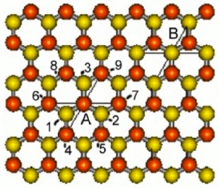
Figure 1: (Color online) Neighbors of a given atom $A$. Only the neighbors labelled 1, 2, 3, 4, 6, 7 and 9 are affected by the difference operators $T$, $H$ and $D$ used in our discrete elasticity model.

In continuum mechanics, dislocations are usually described by the equations of linear elasticity with singular sources whose supports are the dislocation lines. To describe dislocations in 2D graphene, we should have a more detailed theory which can be used to regularize the corresponding point singularities. It is possible to use ab initio theories as regularizers but, provided dislocations are sparse and far from each other, there is a much more economic and insightful alternative. We can discretize appropriately linear elasticity on the hexagonal lattice and then periodize the resulting linear lattice model to allow dislocation gliding. The resulting model equations for the displacement vector $(u^{\prime}(n,t),v^{\prime}(n,t))$ (written in primitive coordinates) are Carpio and Bonilla (2008):

$${\rho a^{2}\over 2}{\partial^{2}u^{\prime}\over\partial t^{2}}={\lambda+\mu\over 3}\,[(H-D)u^{\prime}+(2H+D)v^{\prime}]+T[(\lambda+3\mu)u^{\prime}-2(\lambda+\mu)v^{\prime}],$$ (1)

$${\rho a^{2}\over 2}{\partial^{2}v^{\prime}\over\partial t^{2}}={\lambda+\mu\over 3}\,[(H+2D)u^{\prime}+(D-H)v^{\prime}]+T[(\lambda+3\mu)v^{\prime}-2(\lambda+\mu)u^{\prime}].$$ (2)

where $n=(x,y)$ is a node $A$ or $B$ on one of the two sublattices in Figure 1, $\rho$ is the mass density, $a$ is the lattice constant and $\lambda$ and $\mu$ are the Lamé coefficients which can be obtained from the elastic constants of (isotropic) graphite in its basal plane, $C_{11}=C_{12}+2C_{66}=1060$ GPa, $C_{12}=\lambda=180$ GPa, $C_{66}=\mu=440$ GPa.Blakeslee et al. (1970) Note that $u^{\prime}=(u-v/\sqrt{3})/a$ and $v^{\prime}=2v/(a\sqrt{3})$ are nondimensional because the components of the displacement vector in cartesian coordinates $(u,v)$ have units of length. The difference operators $T$, $D$ and $H$ act on functions of the coordinates $(x,y)$ of the node $A$ in Fig. 1 according to the formulas:

$$Tu^{\prime} = g(u^{\prime}(n_{1})-u^{\prime}(A))+g(u^{\prime}(n_{2})-u^{\prime}(A))+g(u^{\prime}(n_{3})-u^{\prime}(A)),$$ (3)

$$Hu^{\prime} = g(u^{\prime}(n_{6})-u^{\prime}(A))+g(u^{\prime}(n_{7})-u^{\prime}(A)),$$ (4)

$$Du^{\prime} = g(u^{\prime}(n_{4})-u^{\prime}(A))+g(u^{\prime}(n_{9})-u^{\prime}(A)),$$ (5)

where $g$ is a periodic function, with period one, and such that $g(x)\sim x$ as $x\to 0$. Note that the operator $T$ involves finite differences with the three next neighbors of $A$ which belong to sublattice 2, whereas $H$ and $D$ involve differences between atoms belonging to the same sublattice along the primitive directions $\mathbf{a}$ and $\mathbf{b}$, respectively. See Figure 1. The same formulas hold if $(x,y)$ is an atom $B$ in the other sublattice. Far from dislocation cores, the finite differences are very small and close to the corresponding differentials. If we Taylor expand these finite difference combinations about $(x,y)$, insert the result in (1) and (2) and write the displacement vector in cartesian coordinates, we recover the equations of linear elasticity Carpio and Bonilla (2008).

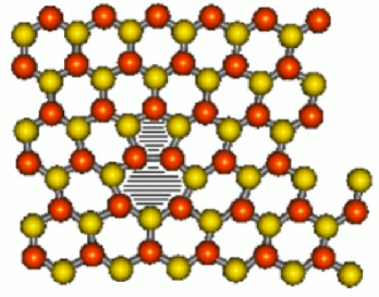
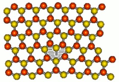
Figure 2: (Color online) Structure of the glide (left) and shuffle (right) dislocations in the planar graphene lattice.

The role of the periodic function $g$ is to allow dislocation gliding Carpio and Bonilla (2003, 2005); Bonilla et al. (2007). When a defect moves, a few atoms change some of their nearest neighbors. We use the periodized difference operators $T$, $D$ and $H$ in (1) - (2) instead of solving discrete elasticity with an updating algorithm that keeps track of neighbor change. The equations of periodized discrete elasticity (1) - (2) regularize linear elasticity and allow for dislocation motion and for dislocation nucleation Plans et al. (2008).

How do we find the defects in graphene that correspond to different edge dislocations? We first substitute $(x,y)$ in the elastic field of a dislocation (such as the edge dislocation of page 57 of Ref. Nabarro, 1967) by $x=a\,(x^{\prime}_{0}+l+y^{\prime}_{0}/2+m/2)$, $y=a\sqrt{3}\,(y^{\prime}_{0}+m)/2$. $l$ and $m$ are integer numbers that allow the resulting displacement vector to be a vector function of lattice points, which we denote by ${\bf U}(l,m)$. The primitive coordinates $x^{\prime}=x^{\prime}_{0}+l$, $y^{\prime}=y^{\prime}_{0}+m$ are centered in an appropriate point $(x^{\prime}_{0},y^{\prime}_{0})$ which is different from the origin to avoid the singularity in the elastic field to coincide with a lattice point. We now solve an overdamped periodized discrete elasticity model (in which second order time derivatives are replaced by first order ones) with a boundary condition given by ${\bf U}$ and with an initial condition also given by ${\bf U}$. After a certain relaxation time, the solution of the model evolves to a stable stationary configuration which depends on the location of the origin $(x^{\prime}_{0},y^{\prime}_{0})$ and on ${\bf U}$. This stable configuration is also a stable configuration of the original equations of the model (with inertia).

By using the method just sketched, we have obtained that the same dislocation solution of the equations of elasticity may have different cores, which is a familiar fact in crystals with diamond structure and covalent bonds, such as silicon; see page 376 in Ref. Hirth and Lothe (1968). The stable configurations corresponding to one edge dislocation are pentagon-heptagon defects (‘glide’ dislocations) if the singularity is placed between two atoms that form any non-vertical side of a given hexagon. If the singularity is placed in any other location different from a lattice point, the core of the singularity forms a ‘shuffle’ dislocation: an octagon having one atom with a dangling bond, as shown in Fig. 2.

If we use the elastic field of an edge dislocation dipole as initial and boundary condition, there are again different stable configurations depending on how we place the dislocation cores. An edge dislocation dipole is formed by two edge dislocations with Burgers vectors in opposite directions. Let ${\bf E}(x,y)$ be the displacement vector corresponding to the edge dislocation. If ${\bf U}={\bf E}(x-x_{0},y-y_{0}-l/2)-{\bf E}(x-x_{0},y-y_{0})$ ($l=a/\sqrt{3}$ is the hexagon side in terms of the lattice constant $a$), the stable stationary configuration is that of a vacancy. If ${\bf U}={\bf E}(x-x_{0},y-y_{0}-l)-{\bf E}(x-x_{0},y-y_{0})$, a dynamically stable divacancy (formed by one octagon and two adjacent pentagons) results. An initial configuration corresponding to a Stone-Wales defect, ${\bf E}(x-x_{0}-a,y-y_{0})-{\bf E}(x-x_{0},y-y_{0})$, is dynamically unstable: at zero applied stress, the two component edge dislocations glide towards each other and annihilate. If a shear stress is applied in the glide direction of the two edge dislocations comprising the SW defect, these defects either continue destroying themselves or, for large enough applied stress, are split in their two component heptagon-pentagon defects that move in opposite directions Carpio and Bonilla (2008).

Instead of a dislocation dipole, our initial configuration may be a dislocation loop, in which two edge dislocations with opposite Burgers vectors are displaced vertically by one hexagon side: ${\bf E}(x-x_{0}-a,y-y_{0})-{\bf E}(x-x_{0},y-y_{0}-l)$ ($l=a/\sqrt{3}$ is the length of the hexagon side). In principle, the dislocation loop could evolve to an inverse SW defect (7-5-5-7). Instead, this initial configuration evolves towards a single octagon. If we displace the edge dislocations vertically by $l/2$, ${\bf E}(x-x_{0}-a,y-y_{0})-{\bf E}(x-x_{0},y-y_{0}-l/2)$, the resulting dislocation loop evolves towards a single heptagon defect Carpio and Bonilla (2008).

III Electronic properties.

The electronic structure of the solids and most of their low energy properties are dictated by the position of the Fermi surface, its shape, and the amount of electrons available at energies close to it. In the independent electron approximation, valid when the kinetic energy of the electrons is much larger than their mutual interactions, electronics is well described by band theory. The latter gives two main outputs: geometry of the Fermi surface and density of states at the Fermi level Kittel (1996).

The tight-binding approximation assumes that the electrons in the crystal behave much like an assembly of constituent atoms. It works by replacing the many-body Hamiltonian operator by a matrix Hamiltonian. The solution to the time-independent single electron Schrödinger equation is well approximated by a linear combination of atomic orbitals. These form a minimal set of short range basis functions $\phi_{i}$ -that we do not need to specify- and the full wave function at site i is given by

$$\Psi_{i}=\sum_{ij}C_{ij}\phi_{j}.$$

The electron density at a lattice site $pq$ can be computed as

$$P_{pq}=2\sum_{k}^{occ}\sum_{pq}C_{pk}C^{*}_{qk}.$$

The tight binding energy is given by

$$E=\sum_{pq}P_{pq}h_{pq}=2\sum_{k}^{occ}\sum_{pq}C_{pk}C^{*}_{qk}h_{pq},$$

where $h{pq}$ is the element of the matrix Hamiltonian.

The advantage of the method is that matrix elements

$$h_{pq}=<p|H|q>=\int d{\bf r}\phi^{*}_{p}({\bf r})H\phi_{q}({\bf r}),$$

$$S_{pq}=<\phi_{p}|\phi_{q}>=\int d{\bf r}\phi^{*}_{p}({\bf r})\phi_{q}({\bf r}),$$

are not explicitly calculated but approximated by phenomenological parameters that depend on the geometry of the lattice and the nature of the orbitals.

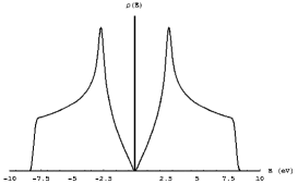
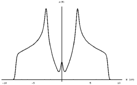
Figure 3: Total density of states. Left Panel: Clean graphene. Right Panel: Graphene ribbon with zigzag edges.

The full strength of the tight binding approximation is related with the perfect -discrete- translational invariance of the periodic lattice. The use of Bloch wave functions in Fourier space allows a full description of the dispersion relation with the only input of the overlapping integrals that can be indirectly deduced from experiments. Since we are going to treat lattice defects that break translational invariance we will stay in real space and adopt the simplest possible approximation: site energies are set to zero and overlapping integrals are non-zero only for nearest neighbor atoms. The hopping integral in graphene is estimated to be of the order of $t\sim 2.7eV$. In summary, and in a very general sense, the electronic structure within the tight binding approximation is obtained simply by defining a lattice with links, and diagonalizing the Hamiltonian, a matrix with elements $h_{ij}$ equal to $t$ if atom $i$ is linked to $j$ and zero otherwise. This is the calculation that we have performed.

A full analysis of the tight binding structure of graphene can be seen in the original paper Wallace (1947) and in the reference book Saito et al. (1998). Its main outcome is that the Fermi surface reduces to two points and the density of states vanishes at the Fermi energy which, in turn, determines the semimetallic character of the material. The density of states is very important to characterize the electronic and transport properties of the samples. Disorder can open a gap or, more often, induce a finite density of states. Real samples have localized states at (or about) zero energy which are induced close to edges, vacancies, ad-atoms or other defects. These midgap states can form very narrow bands where the electronic interactions become important and may lead to electronic instabilities, particularly ferromagnetism Guinea et al. (2008).

The density of states of an ideal graphene sheet is shown in the left panel of Fig. 3. It vanishes at the Fermi energy what determines the semi-metallic character of the material. Defects in the lattice very often induce states at zero energy. An important class is that of edge states induced by certain boundaries in finite lattices or real samples (graphene nanoribbons). Zigzag (armchair) edges can be seen in the horizontal (vertical) borders in Fig. 1. Zigzag edges with uncoordinated atoms belonging to the same sublattice induce a number of zero energy edge states proportional to the amount of unpaired lattice sites Fujita et al. (1996). They are important in potential applications. These energy states are localized at the edges as it can be seen in the local DOS of Fig. 5. When studying electronic properties via numerical simulations, it is important to disentangle the low energy effects coming from the boundary from those which are intrinsic to the defects under study. The density of states of a graphene nanoribbon with zigzag edges is shown for comparison in the right panel of Fig. 3.

Electronic structure of single dislocations

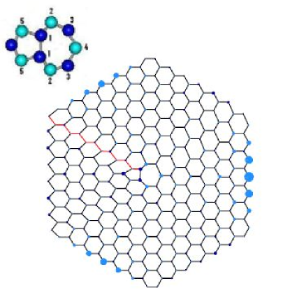
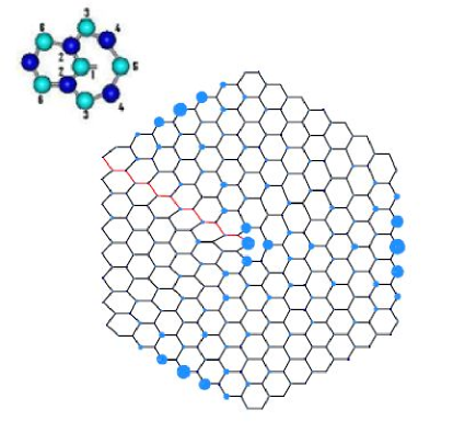
Figure 4: (Color online) Left: Lattice structure and charge density for a low energy eigenstate in the presence of a glide dislocation shown in the inset. Right: Same for the shuffle dislocation.

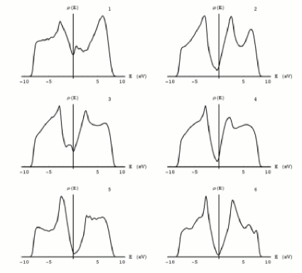
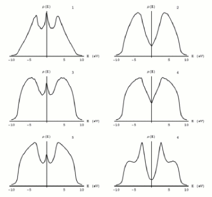
Figure 5: Left: For the graphene sample with a glide dislocation depicted in Fig. 4, local density of states at the numbered sites around the defect shown in the inset of Fig. 4. Right: Same for the sample with a shuffle dislocation.

As discussed in section II, the “glide” and “shuffle” dislocations shown in Fig. 2 are stable in the graphene sheet. We have performed a tight binding calculation for these two types of dislocations. Fig. 4 shows the configuration of the lattice for the dislocations depicted in the inset where the atoms that constitute the defect are numbered. The extra rows of atoms characteristic of these edge dislocations are shown in red. The area of the circles is proportional to the squared wave function for one of the lowest energy eigenvalues. The extra charge appearing at the shuffle dislocation is due to the dangling bond attached to it.

In Fig. 5, we show the local density of states (LDOS) for the five sites around the defect numbered in the inset of Fig. 4 and for an extra site located at a certain distance from the defect. The LDOS is drastically distorted at the defects but rapidly recovers the normal shape away from the center of the defect. The pentagon-heptagon pair (glide dislocation) breaks the electron-hole symmetry of the lattice but the corresponding LDOS resembles that of the perfect lattice shown in fig. 3. The LDOS at zero energy is not zero, but it has a minimum in all cases. The sixth graph shows the LDOS at an atom located six lattice units apart from the defect. This is the distance at which the influence of the dislocation ceases to be noticeable.

The shuffle dislocation has a more pronounced effect on the LDOS. As can be seen in Fig.  5, at zero energy there appear sharp peaks at the position of the dangling bond atom and at neighboring sites of the same sublattice whereas dips in the LDOS appear at the sites of the opposite sublattice. The distortion in the LDOS decays faster with distance in the case of a shuffle dislocation than in the case of a heptagon-pentagon pair. The right panel of Fig. 5 shows that the density of states of the perfect lattice is already recovered at position 6 of the inset in Fig. 4, one lattice distance away from the defect. The mid gap state induced by the defect is strongly peaked at the defect position, similarly to what happens with the zigzag edges states. This type of dislocation does not break the electron hole symmetry of the lattice.

Defects of Stone Wales type

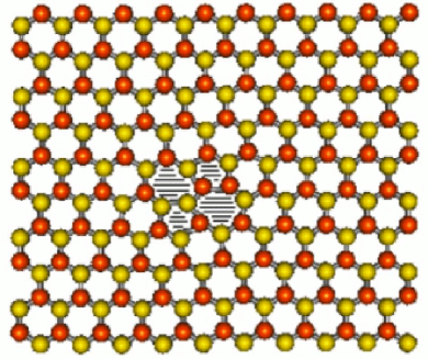
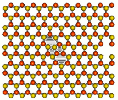
Figure 6: (Color online) Left: Lattice structure of a Stone Wales defect. Right: Same for the dislocation dipole described in the text.

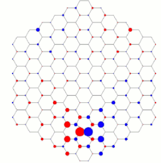
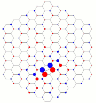
Figure 7: (Color online) Left: Lattice structure and charge density for the fourth positive-energy eigenstate in the presence of a Stone Wales defect. Right: Same for the dislocation dipole described in the text.

One of the best studied defects in the carbon nanotube literature is the Stone Wales (SW) defect Slonczewski and Weiss (1958). It consists of two heptagon-heptagon pairs that can be obtained by a ninety degree rotation of a lattice bond. The resulting structure is shown in the left hand side of fig. 6. These defects play a very important role in the surface reconstruction of irradiated nanotubes Ajayan et al. (1998) and affect their mechanical properties. From the standpoint of elasticity, they can be seen as two identical edge dislocations that have opposite Burgers vectors and share the same glide line. They have been found to be dynamically unstable: their component edge dislocations glide towards each other and annihilate, leaving the undistorted lattice as the final configuration Carpio and Bonilla (2008). A type of defect whose final configuration is very similar – two heptagon-pentagon pairs – is shown in the right panel of Fig. 6. It is a dislocation dipole whose two edge dislocations with opposite Burgers vectors are displaced vertically by one lattice unit. By solving the periodized discrete elasticity model of Section II, we can show that this configuration is dynamically stable. The electronic structure of these two defects is depicted in Figs. 7 and 8. These dipole defects induce a stronger local distortion of the charge density than single dislocations. While the real SW defect does not alter the structure of the lattice edges, the other dislocation dipole has two extra atoms as compared to the perfect lattice and therefore it alters the structure of its edges. This is clearly visible in Fig. 6. The presence of these defects can affect the electronic properties of real samples.

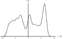
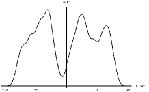
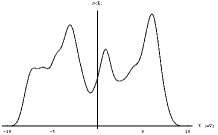
Figure 8: From left to right: Local density of states of a real SW defect at the site shared by the two adjacent pentagons and at its nearest neighbor. LDOS of the dislocation dipole discussed in the text at the site shared by the two heptagons and at its nearest neighbor.

IV Conclusions and discussion

We have used a regularization of the continuum elasticity on the honeycomb lattice to explore the stability and evolution of topological defects. Two types of dislocations are stable: pentagon-heptagon pairs (‘glide’ dislocations) and ‘shuffle’ dislocation: an octagon having one atom with a dangling bond. They are shown in Fig. 2. Both defects induce distortions in the local density of states at low energies that decay rapidly with the distance to the defect. The presence of a dangling bond in the shuffle dislocations drastically enhances these effects but, as in the case of zigzag states, the low energy states are very localized.

The main physical effect of the shuffle dislocations will be related with the nucleation of magnetic moments at the dangling bonds. Work in this direction is in progress.

Regarding configurations of edge dislocation dipoles in discrete elasticity, vacancies and di-vacancies are stable but Stone-Wales defects are dynamically unstable. This situation is to be confronted with what happens in the carbon nanotubes where SW defects are stable. This points to the idea that curvature and geometry play a role in their stabilization. We are also working in this direction.

A defect similar to the SW consists of a dislocation dipole whose component dislocations are displaced one lattice unit. This defect is dynamically stable and can give rise to a large local distortion of the electronic density. The defects discussed in this work are very likely to be present in real samples of both graphene and nanoribbons. They will affect the transport properties of the samples and they will also alter the configuration of the sample edges. This must be taken into consideration in the cases when perfect tayloring of the edges is important.