Hybrid planar FEM in magnetoresonance regime: control of dynamical chaos

Abstract

We establish the influence of nonlinear electron dynamics in the magnetostatic field of a hybrid planar free-electron maser on its gain and interaction efficiency. Even for the ‘ideal’ undulator magnetic field the presence of uniform longitudinal (guide) magnetic field potentially leads to the existence of chaotic zone around certain (magnetoresonant) value of the guide magnetic field. The width of the chaotic zone is given by the Chirikov resonance-overlap criterion applied to the normal undulator and cyclotron frequencies with respect to the coupling induced by the undulator magnetic field. Using analytical asymptotically exact solutions for trajectories of individual test electrons, we show that the magnetoresonant multiplier in electron trajectories is also present in the expression for the gain. The same Chirikov resonance-overlap criterion allows us to estimate analytically the maximal magnetoresonant gain of a hybrid planar free-electron maser showing that, in spite of the well-known drop in the gain for the exact magnetoresonance, the operation regime in the zone of regular dynamics slightly above the magnetoresonant value of the guide magnetic field is the preferable one.

I Introduction

Starting with the successful experiment Sprangle and Granatstein (1978); Parker et al. (1982), previous three decades have witnessed a spectacular development of theory and experiment of free-electron maser with guide (uniform longitudinal) magnetic field (hybrid FEM). Utilizing the Doppler frequency upshift, free-electron masers and lasers posses a unique property to amplify and generate coherent electromagnetic radiation across nearly complete electromagnetic spectrum: from radio waves to vacuum ultraviolet Andruszkow et al. (2000). An interest to the hybrid FEM is reinforced by a promise to attain a substantial microwave power level (up to a few gigawatts) in their planar configuration because of the use of superwide sheet electron beams (e.g., in Agafonov et al. (1998) emission and transport of a 140 cm-wide, 20 kA and 2 MeV sheet electron beam for purported FEM applications was reported). Sheet electron beams allow one to weaken restrictions on the maximal aggregate beam current posed by space charge effects while reaching the current values of about 30 $\div$ 50 kA. This makes the hybrid planar FEM one of the most attractive sources of powerful electromagnetic radiation in the Terahertz Gap: the frequency range from 0.3 to 3 THz.

In pioneering works Louisell et al. (1979); Freund et al. (1981); Kokhmanskii and Kulish (1984); Masud et al. (1986); Ginzburg and Novozhilova (1986) analytical investigations of stationary regimes of microwave amplification and generation in a hybrid FEM were carried out; later these results were refined mainly through numerical simulations. Experimentalists Conde and Bekefi (1991); Viktorov et al. (1991); Sakamoto et al. (1993); Bratman et al. (1996) reported a considerable loss of electron beam current and microwave power for a hybrid FEM for a certain range of values of the guide magnetic field. A study of chaotic particle dynamics in free-electron lasers was undertaken in papers Chen and Donaldson (1990, 1991), where the authors investigated effects of high-current (high-density) regime and the transverse spatial gradients in the applied wiggler magnetostatic field. Nevertheless, to the present day there still exist some fundamental questions, which either have no answers or only partial ones (cf. (Freund and Antonsen, 1995, pp. 430-439)): under what conditions motion of an individual test electron becomes chaotic in the presence of guide magnetic field; what does influence the width of dynamical chaos zone around the magnetoresonant value (the undulator frequency is approximately equal to the cyclotron frequency) of the guide magnetic field; which maximal portion of initial kinetic energy from the longitudinal motion can be transferred to the transversally-vibrational motion (in an FEM the transfer of beam energy from longitudinal constant motion to the microwave field takes place indirectly through coupling of transversally-vibrational degrees of freedom to the microwave); does such an interaction with the microwave cause any widening of the chaotic dynamics zone; and, finally, what does define the maximal value of the gain under the conditions of the magnetoresonance?

We focus our attention on the operation of FEM around the magnetoresonant regime caused by the guide magnetic field usually used in FEM setups to enhance the efficiency of beam-microwave interaction and provide transverse confinement of electron beam. The study is based upon analytical asymptotically exact expressions for electron trajectories developed recently Yefimov et al. (2004); Goryashko et al. (2006a) as well as on the use of direct numerical simulations. More specifically, in the adopted approach we highlight the fundamental role of nonlinear dynamical system describing motion of electrons in the combined magnetostatic spatially periodic (undulator) and uniform guide magnetic field.

The next Section contains nonlinear and linearized in the microwave field self-consistent systems of equations governing a hybrid planar FEM amplifier. In Section III, we find asymptotically exact solutions of equations of motion of an individual test electron in the magnetostatic field of a hybrid planar FEM and study their properties. Section IV contains derivation of dispersion equations and calculation of magnetoresonant growth rates. A comparison with direct numerical simulations of self-consistent nonlinear system of governing equations is presented in Section V. The article ends with the Summary and Discussions Section.

II Governing Equations

We regard that at the entrance of the interaction region (cross-section $z=0$) of a hybrid planar FEM the electron beam is continuous and unmodulated. In the amplifier regime there also is a seed microwave signal. It can be shown that for a regular electrodynamics structure the microwave field and electron beam current density in the interaction region are periodic functions of time. Neglecting temporal harmonics generation, we will assume that there occurs resonant interaction only with one spatial harmonic of the microwave field. Under such assumptions the microwave field in an ideally conducting regular waveguide with the electron beam

$$\begin{split}\vec{E}(\vec{r},\!t)&\!\!\approx\!\mathrm{Re}\{C\vec{E}^{0}(\vec{r},\!t)\}\!\!=\!\mathrm{Re}\{C(z)\vec{e}(\vec{r}_{\perp})e^{-i(\omega t-k^{0}_{z}z)}\},\\ \vec{B}(\vec{r},\!t)&\!\!\approx\!\mathrm{Re}\{C\vec{B}^{0}(\vec{r},\!t)\}\!\!=\!\mathrm{Re}\{C(z)\vec{b}(\vec{r}_{\perp})e^{-i(\omega t-k^{0}_{z}z)}\}\end{split}$$ (1)

differs from that of without the electron beam only by an amplitude multiplier $C(z)$ ($\vec{E}^{0}(\vec{r},t)$ and $\vec{B}^{0}(\vec{r},t)$ obey homogeneous Maxwell’s equation); $\vec{e}(\vec{r}_{\perp})$ and $\vec{b}(\vec{r}_{\perp})$ are the membrane eigenfunctions of the coordinates $\vec{r}_{\perp}=(x,y)$ in the waveguide cross-section $S$ (microwaves and the electron beam propagate in the positive direction of the $z$-axis, see Fig. 1); $k^{0}_{z}$ is the ‘cold’ propagation constant of the eigenwave.

In the case of low-density electron beam, one can neglect its space-charge and, by averaging on the electrons’ entrance phase, reduce the problem of interaction of electron beam with a seed synchronous microwave of frequency $\omega$ to the task of solving a single-particle equations of motion for arbitrary entrance time $t_{e}$ and Maxwell’s equations in the form of Kisunko-Vainshtein’s equations of excitation for regular waveguides Kisunko (1949); Vainshtein and Solntsev (1973). It is exactly in this manner a highly successful theory of the gyrotron was initially developed by Gaponov Gaponov (1961).

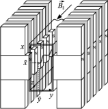
Figure 1: Schematic drawing of rectangular waveguide with mounted permanent magnet planar undulator immersed in the uniform longitudinal (guide) magnetic field.

Following (Vainshtein and Solntsev, 1973, p. 200) (see also Gover (1995)), let us write the self-consistent nonlinear system of equations in the form:

$$m_{e}\frac{d(\gamma\vec{v})}{dt} = e\vec{E}+\frac{e}{c}[\vec{v}\times(\vec{B}_{p}+\vec{B})],$$ (2a)

$$\frac{dC}{dz} = -\frac{\omega}{2\pi P_{0}}\int\limits_{S}\!\!\!\int\limits_{-\pi/\omega}^{\pi/\omega}\!\!\!\!(\vec{j}\cdot(\vec{E}^{0})\raisebox{4.30554pt}[0.0pt][0.0pt]{\scriptsize$\ast$})e^{i\omega t}dtdS,$$ (2b)

where

$$\vec{j}(\vec{r},t) = e\!\!\sum\limits_{k}\delta(\vec{r}-\vec{r}^{\,k})\vec{v}^{\,k},$$

$$P_{0} = \frac{c}{8\pi}\mbox{Re}\int_{S}([\vec{e}(\vec{r}_{\perp})\times\vec{b}^{\ast}(\vec{r}_{\perp})]\cdot\vec{e}_{z})dS.$$

Here $m_{e}$ and $e$ are the electron rest mass and charge, respectively; $c$ is the speed of light; $\vec{v}=d\vec{r}/dt$, $\gamma=(1-\vec{v}\,^{2}/c^{2})^{-1/2}$ is the relativistic factor; $\vec{j}(\vec{r},t)$ is the electron current density; $\vec{r}^{\,k}(t)=\vec{r}(t,t^{k}_{e})$ and $\vec{v}^{\,k}(t)=\vec{v}(t,t^{k}_{e})$ are the coordinates and velocity of a $k$’s electron, which entered the interaction region at the moment of time $t^{k}_{e}$; the star (^∗) denotes complex conjugation; $\vec{e}_{z}$ is the unit vector along the $z$-axis; the overbar in equation (2b) stands for the time average, which is effectively reduced to the averaging over the electrons’ entrance phase. Initial conditions for system (2) consist in the specification of coordinates, velocities and the amplitude of microwave field at the entrance to the interaction region: $\vec{r}\,(t_{e},t_{e})=(\bar{x},\bar{y},0)$, $\vec{v}\,(t_{e},t_{e})=(V_{x},V_{y},V_{\|})$ and $C(0)=C_{0}$.

Magnetostatic field $\vec{B}_{p}(\vec{r})$ consists of a guide (uniform longitudinal) magnetic field $\vec{B}_{\|}$ and planar spatially periodic undulator magnetic field $\vec{B}_{w}(\vec{r})=$ $-B_{\perp}(0,\cosh(2\pi[y-b^{\prime}/2]/\lambda_{w})\sin(2\pi z/\lambda_{w}),\sinh(2\pi[y-b^{\prime}/2]/\lambda_{w})\cos(2\pi z/\lambda_{w}))$. Having the primary goal in demonstration of underlying physics, we intentionally consider a simplest possible model of a hybrid planar FEM (which accounts for the undulator through only one component of its spatially periodic magnetic field taken in the limit $2\pi[y-b^{\prime}/2]/\lambda_{w}$ $\ll$ $1$):

$$\vec{B}_{p}=(0,-B_{\perp}\sin(2\pi z/\lambda_{w}),-B_{\|}),$$ (3)

where $B_{\perp}$ is a constant amplitude Sakamoto et al. (1993); Cheng et al. (1996) and $b^{\prime}$ is the undulator gap width. However, the developed approach can be extended straightforwardly on ‘realisable’ undulator/wiggler magnetic fields and space charge dominated beams.

In order to explore analytically the linear stationary regime of amplification, we linearize equations (2) in the microwave fields $\vec{E}$ and $\vec{B}$ ($B_{\|}$, $B_{\perp}$ $\gg$ $c|\vec{E}|/|\vec{v}|$, $|\vec{B}|$). Trajectory of an electron is primarily given by its motion in the magnetostatic field

$$\vec{r}(t,t_{e})\equiv\vec{r}(\tilde{t},t_{e})=\vec{r}_{0}(\tilde{t})+\mathrm{Re}\{\vec{r}_{1}(\tilde{t})e^{i\omega t_{e}}\}\,\,\,\,(|\vec{r}_{0}|\gg|\vec{r}_{1}|);$$

$\tilde{t}=t-t_{e}$ stands for the transit time of an electron. We also hold that $C(z)$ is a slow function of $z$. In the zeroth-order in the microwave field approximation system (2) reduces to equations of motion in the magnetostatic field

$$m_{e}\frac{d(\gamma_{0}\vec{v}_{0})}{d\tilde{t}}=\frac{e}{c}\,[\vec{v}_{0}\times\vec{B}_{p}(\vec{r}_{0})],$$ (4)

where $\vec{v}_{0}=d\vec{r}_{0}/d\tilde{t}$ and $\gamma_{0}=(1-\vec{v}_{0}^{\,2}/c^{2})^{-1/2}$. It then immediately follows that in this approximation the total kinetic energy is conserved (i.e. $\gamma_{0}=$ const; $\vec{v}_{0}^{\,2}=\vec{v}^{\,2}(t_{e},t_{e})\equiv V_{x}^{2}+V_{y}^{2}+V_{\|}^{2}$), which greatly simplifies the analysis of system (4). It should be emphasized that properties of solutions to equations (4) are fundamental to the consideration of microwave amplification and generation in a FEM Friedland and Hirshfield (1980); Colson (1981); Freund et al. (1981). In the first order (linear) approximation in the microwave field, we obtain a coupled system of equations for $\vec{r}_{1}$ and linearized equations of excitation

$$m_{e}\gamma_{0}\frac{d}{d\tilde{t}}\Big{[}\vec{v}_{1} + \gamma_{0}^{2}\vec{v}_{0}\frac{(\vec{v}_{0}\cdot\vec{v}_{1})}{c^{2}}\Big{]}=eC\vec{F}+$$ (5a)

$$\frac{e}{c}\{[\vec{v}_{1} \times \vec{B}_{p}(\vec{r}_{0})]+[\vec{v}_{0}\times(\vec{r}_{1}\cdot\vec{\nabla})\vec{B}_{p}(\vec{r})|_{\vec{r}=\vec{r}_{0}}]\},$$

$$\frac{dC}{d\tilde{t}} = -\frac{i\omega|I_{0}|}{4P_{0}}(\vec{r}_{1}\cdot\vec{F}^{*}),$$ (5b)

where

$$\vec{F}(\tilde{t}) = \vec{f}(\vec{r}_{0\perp},\vec{v}_{0})e^{-i(\omega\tilde{t}-k^{0}_{z}z)},$$

$$\vec{f}(\vec{r}_{0\perp},\vec{v}_{0}) = \vec{e}\,(\vec{r}_{0\perp})+c^{-1}[\vec{v}_{0}\times\vec{b}(\vec{r}_{0\perp})].$$

Here $\vec{v}_{1}=d\vec{r}_{1}/d\tilde{t}$, $I_{0}$ is the electron beam current at the entrance to the interaction region and $\vec{F}(\tilde{t})$ is the microwave force estimated at the unperturbed electron trajectory.

III Magnetostatic Resonance: Energy Transfer and Dynamical Chaos

In this Section we examine dynamics of an individual test electron in the magnetostatic field (3) given by system (4). In components the equations have the form:

$$\ddot{x}_{0} - \omega_{\|}\dot{y}_{0}={}-\omega_{\perp}\dot{z}_{0}\sin(\omega_{0}z_{0}/V_{\|}),$$

$$\ddot{y}_{0} + \omega_{\|}\dot{x}_{0}=0,$$ (6)

$$\ddot{z}_{0} = \omega_{\perp}\dot{x}_{0}\sin(\omega_{0}z_{0}/V_{\|}),$$

where $\omega_{0}=2\pi V_{\|}/\lambda_{w}$ is the undulator frequency and $\omega_{\perp,\|}=|e|B_{\perp,\|}/(m_{e}c\gamma_{0})$; the overdots denote differentiation with respect to the transit time $\tilde{t}$. One can easily find two first integrals of this nonlinear dynamical system just by integrating its first two equations and take the energy conservation law as the third linearly independent one

$$\dot{x}_{0}-\omega_{\|}y_{0}-(2\pi)^{-1}\omega_{\perp}\lambda_{w}\cos(\omega_{0}z_{0}/V_{\|}) \equiv F_{1}=\mbox{const},$$

$$\dot{y}_{0}+\omega_{\|}x_{0}\equiv F_{2}=\mbox{const},\,\,\dot{z}_{0}^{2}+\dot{x}_{0}^{2}+\dot{y}_{0}^{2} \equiv F_{3}=\mbox{const}.$$

Although, system (6) cannot be integrated in quadratures everywhere because it possesses non-zero Lyapunov exponents (see below Fig. 7 and (Lieberman and Lichtenberg, 1992, p. 208)). It should be noted that out of six quantities $\lambda_{w}$, $B_{\perp}$, $B_{\|}$, $V_{\|}$, $V_{x}$ and $V_{y}$ only four their dimensionless combinations $\varepsilon=\omega_{\perp}/\omega_{0}\equiv c\mathcal{K}/(\gamma_{0}V_{\|})$ ($\mathcal{K}$ is the conventional undulator parameter), $\sigma_{0}=\omega_{\|}/\omega_{0}$, $V_{x}/V_{\|}$ and $V_{y}/V_{\|}$ define the behavior of nonlinear dynamic system (6). Solution to system (6) can be obtained by the use of a method of Lindshtedt Linshtedt (1883); Blaquiere (1966) of asymptotic expansion of trajectory and frequencies in the small parameter $\varepsilon$ (see Yefimov et al. (2004) for a detailed exposition of the method in the case $V_{x}=V_{y}=0$). To the order $o(\varepsilon^{2})$ the velocity components read:

$$\dot{x}_{0}(\tilde{t}) = \hphantom{-}V_{\perp}\cos(\Omega_{\|}\tilde{t}-\psi)+\bar{v}_{\|}\frac{\omega_{\perp}\Omega_{0}}{\Omega_{0}^{2}-\Omega_{\|}^{2}}\Bigl{[}\cos(\Omega_{0}\tilde{t})-\cos(\Omega_{\|}\tilde{t})\Bigr{]},$$

$$\dot{y}_{0}(\tilde{t}) = -V_{\perp}\sin(\Omega_{\|}\tilde{t}-\psi)+\bar{v}_{\|}\frac{\omega_{\perp}\Omega_{0}}{\Omega_{0}^{2}-\Omega_{\|}^{2}}\Bigl{[}\sin(\Omega_{\|}\tilde{t})-\frac{\Omega_{\|}}{\Omega_{0}}\sin(\Omega_{0}\tilde{t})\Bigr{]},$$ (7)

$$\dot{z}_{0}(\tilde{t}) = \bar{v}_{\|}-V_{\perp}\omega_{\perp}\Bigl{[}\frac{\cos([\Omega_{0}-\Omega_{\|}]\tilde{t}+\psi)}{2(\Omega_{0}-\Omega_{\|})}+\frac{\cos([\Omega_{0}+\Omega_{\|}]\tilde{t}-\psi)}{2(\Omega_{0}+\Omega_{\|})}\Bigr{]},$$

where $V_{\perp}=(V_{x}^{2}+V_{y}^{2})^{1/2}$, $\sin{\psi}=V_{y}/V_{\perp}$, $\bar{v}_{\|}=\kappa V_{\|}$, $\Omega_{0}=\kappa\omega_{0}$ and $\Omega_{\|}=\sigma\omega_{\|}/\sigma_{0}$. Here $\kappa$ and $\sigma$ to the order $o(\varepsilon^{3})$ are given by the following self-consistent system of algebraic equations:

$$\kappa=1+\frac{\varepsilon V_{x}}{V_{\|}(\kappa^{2}-\sigma^{2})}-\varepsilon^{2}\Bigr{[}\frac{3\kappa^{2}+\sigma^{2}}{4(\kappa^{2}-\sigma^{2})^{2}}-\frac{V_{x}^{2}(8\kappa^{4}-13\kappa^{2}\sigma^{2}+\sigma^{4})}{8V_{\|}^{2}\kappa^{2}(\kappa^{2}-\sigma^{2})^{3}}+\frac{V_{y}^{2}(2\kappa^{4}+11\kappa^{2}\sigma^{2}-\sigma^{4})}{8V_{\|}^{2}\kappa^{2}(\kappa^{2}-\sigma^{2})^{3}}\Bigl{]},\frac{\sigma}{\sigma_{0}}=1+\frac{\varepsilon^{2}(\kappa^{2}+\sigma^{2})}{4(\kappa^{2}-\sigma^{2})^{2}};$$ (8)

$\kappa$ and $\sigma$ are found as functions of $\varepsilon$ and $\sigma_{0}$ with $V_{x}/V_{\|}$ and $V_{y}/V_{\|}$ as parameters. An analytical solution to Eqs. (8) can be found by successive iterations starting with ’non-renormalized’ values $1$ and $\sigma_{0}$ for $\kappa$ and $\sigma$, respectively. It is worth noting that Eqs. (8) order by order in $\varepsilon$ provide cancelation of secular terms in the solution procedure for system (6) (cf. Yefimov et al. (2004), which contains the limit of (8), (III) and (A) for the case $V_{x}=V_{y}=0$). For completeness, expressions for contributions to the velocities (III) of the order $\mathcal{O}(\varepsilon^{2})$ are entered in the AppendixA. Using Eqs. (8), (III) and (A) one can check that $\vec{v}_{0}^{\,2}$ is conserved to the order $o(\varepsilon^{3})$ and is equal to $V_{x}^{2}+V_{y}^{2}+V_{\|}^{2}$ as required by the conservative nature of system (6). It should be also noted that this aggregate solution to the order $o(\varepsilon^{3})$ is valid not only for the ‘ideal’ hybrid planar magnetostatic field (3) but also for its ’realizable’ counterpart involving $\vec{B}_{w}(\vec{r})$. The trajectories of electrons are then given by a straightforward integration.

From (III) and (A) it follows that the motion of electron is a superposition of constant motion with velocity $\bar{v}_{\|}$ and three-dimensional oscillations with normal undulator $\Omega_{0}$ and cyclotron $\Omega_{\|}$ frequencies, which differ from their partial analogues $\omega_{0}$ and $\omega_{\|}$ by ‘renormalization’ multipliers $\kappa$ and $\sigma/\sigma_{0}$. Recall that each subsystem of a nonlinear dynamical system possesses its own (partial) oscillation frequency if interaction between subsystems vanishes. Non-zero interaction modifies those oscillation frequencies by some amount Rabinovich and Trubetskov (1989); Arnold (1993) (represented here by multipliers $\kappa$ and $\sigma/\sigma_{0}$); $\kappa$ also shows what portion of electron initial kinetic energy is transferred to the constant motion.

As $\Omega_{\|}$ tends to $\Omega_{0}$ the amplitudes of transversal and longitudinal oscillations increase. This signifies the existence of an internal resonance Sagdeev et al. (1988), i.e. a resonant transfer of kinetic energy from longitudinal constant motion to transversal and longitudinal oscillatory degrees of freedom. We call this situation magnetostatic resonance or magnetoresonance as is customary in the FEM theory Grossman et al. (1983).

III.1 Zero initial transversal velocity

In the case when initial transversal velocity of electrons vanishes ($V_{x}=V_{y}=0$), the expressions (III), (8) and (A) are greatly simplified. Then, as mentioned above, the single-particle electron dynamics is defined only by two dimensionless quantities $\varepsilon$ and $\sigma_{0}$. To calculate the normal undulator and cyclotron frequencies $\Omega_{0}$ and $\Omega_{\|}$, we need to solve for $\kappa$ and $\sigma$ the system of two algebraic equations (8). To achieve maximal accuracy it turns out advantageous to solve this system numerically and use thus obtained values of $\kappa$ and $\sigma$ in the analytical calculations. In Fig. 2 the results of such a solution are shown in firm lines. For comparison, the result of calculation of $\kappa$ and $\sigma$ via Fourier analysis of direct numerical solution of Eqs. (6) for the velocity components is also given (shown by dots in Fig. 2). In Fig. 3 the graphs of $\kappa$ and $\sigma$ vs. $B_{\|}$ are shown in more details for the guide magnetic field values around the magnetoresonance. At the magnetoresonance $B^{\mathrm{res}}_{\|}\approx 6.67$ kG the normal frequencies $\Omega_{0}$ and $\Omega_{\|}$ experience jumps in order to comply with the conservation of kinetic energy in the dynamical system (6). As $\varepsilon$ grows above a certain threshold value two zones of regular dynamics become separated by a chaotic zone centered about the magnetoresonant value of the guide magnetic field (see Fig. 6). Typical Fourier spectra of velocity are shown in Fig. 4. Away from the magnetoresonant values of the guide magnetic field one can easily identify two distinct frequencies corresponding to $\Omega_{0}$ and $\Omega_{\|}$, their beating frequencies and harmonics. Around the magnetoresonance the spectrum is nearly continuous, which is one of the criteria of dynamical chaos.

Mutual orientation of the undulator and guide magnetic fields causes the kinetic energy transfer from the longitudinal constant motion to undulator vibrational (frequencies $\omega_{0}$ and $\Omega_{0}$) and then to cyclotron vibrational (frequencies $\omega_{\|}$ and $\Omega_{\|}$) degrees of freedom of the nonlinear dynamical system (6); the coupling is provided by the amplitude of undulator magnetic field $B_{\perp}$ ($\varepsilon=\omega_{\perp}/\omega_{0}$). Such a picture allows one two possible ways of energy transfer: at magnetoresonant ($\Omega_{0}\approx\Omega_{\|}$) and non-magnetoresonant ($\Omega_{0}\not\approx\Omega_{\|}$) coupling regimes. Obviously, the magnetoresonant regime requires smaller coupling and may become more advantageous for microwave FEM amplifiers and oscillators. It is then necessary to clarify how accessible are these regimes of FEM operation.

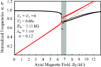
Figure 2: $\kappa$ and $\sigma$ as functions of the guide magnetic field $B_{\|}$. $\kappa$ and and $\sigma$ are depicted in black and red colors, respectively; for reference $\sigma_{0}(B_{\|})$ is given by the chain line. The darkened area corresponds to the zone of chaotic dynamics as given by the Chirikov resonance-overlap criterium (9).

Viewing dynamical system (6) as a nonlinear pendulum with external modulation of its vibration amplitude (cf. the last equation in (6)), one can estimate the condition of appearing of chaotic layer near the separatrix. An analytical estimate is consistent with numerical calculations and coincides with the Chirikov resonance-overlap criterium Chirikov (1979):

$$|\Omega_{0}-\Omega_{\|}|<\omega_{\perp}\,\,(|\kappa-\sigma|<\varepsilon),$$ (9)

i.e. appearance of the chaotic state takes place whenever the difference between normal frequencies of the system becomes less than the coupling. As will be shown in Section IV, the absolute value of the ratio $\omega_{\perp}/(\Omega_{0}-\Omega_{\|})$ (called below the magnetoresonant multiplier) defines the microwave gain. Results of numerical calculations of its maximal value for zones of regular dynamics and practically accessible $\varepsilon(B_{\perp},V_{\|})$ are given in Fig. 5 (for each value one needs to optimize $B_{\|}$; solid and dotted lines correspond to approach of the chaotic zone from low and high values of the guide magnetic field, respectively). This shows that in the magnetoresonant case there exists limitation on the fraction of energy transferred from constant motion to oscillatory (transversal and longitudinal) degrees of freedom posing a fundamental limit on an FEM efficiency. A calculation shows that $\overline{\dot{x}_{0}^{2}(\tilde{t})+\dot{y}_{0}^{2}(\tilde{t}\,)}/\overline{\dot{z}_{0}^{2}(\tilde{t}\,)}\approx 0.48$ (bars denote time averaging). In Fig. 6 we present a contour plot of $\kappa\equiv\bar{v}_{\|}/V_{\|}$ as function of dimensionless coupling $\varepsilon$ and guide magnetic field $\sigma_{0}$. The region of chaotic dynamics is given in black. In Fig. 7 a map of the major Lyapunov exponent as function of $\varepsilon$ and $\sigma_{0}$ is shown. The calculation included a check that the sum of all Lyapunov exponents is equal to zero as mandatory for a conservative dynamical system because of the Liouville theorem.

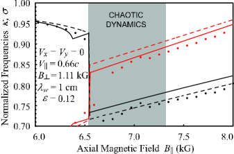
Figure 3: $\kappa$ and $\sigma$ as functions of the guide magnetic field for $B_{\|}$ values around the magnetoresonance. $\kappa$ and and $\sigma$ are depicted in black and red colors, respectively; for reference $\sigma_{0}(B_{\|})$ is given by the chain line.

Figure 4: Logarithmically scaled Fourier spectra of $\dot{x}_{0}$ as function of normalized frequency $\omega/\omega_{0}$. Top figure shows regular dynamics while bottom figure corresponds to chaotic one.

III.2 Non-zero initial transversal velocity;
chaos control

Let us start with demonstration of some features of solutions (III) for a non-zero initial transversal velocity. As follows from (III) and (8), one can have either suppression ($V_{x}>0$) or enhancement ($V_{x}<0$) of the velocity amplitude of cyclotron vibrations, respectively. In particular, for $V_{y}=0$ and $V_{x}=\bar{v}_{\|}\omega_{\perp}\Omega_{0}/(\Omega_{0}^{2}-\Omega_{\|}^{2})$ there occurs a complete, i.e. to the first order in the small parameter $\varepsilon$, suppression of cyclotron vibrations in the transverse to the $z$-axis plane. In Fig. 8 this situation is demonstrated for $V_{y}=0$ and both signs of $V_{x}$ of the same absolute value $|V_{x}|=0.1c$, $V_{\|}=0.66c$, $B_{\perp}=1.11$ kG, the value of $B_{\|}$ is chosen to be $6.67$ kG and corresponds to the magnetoresonance for $V_{x}<0$ (only projections of electron trajectories in the $xy$-plane are shown).

Figure 5: Maximal value of magnetoresonant multiplier as function of dimensionless coupling $\varepsilon$.

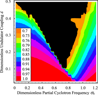
Figure 6: Contour plot of $\kappa\equiv\bar{v}_{\|}/V_{\|}$ as function of dimensionless coupling $\varepsilon$ and guide magnetic field $\sigma_{0}$. The region of chaotic dynamics is given in black.

It should be noted that in general the presence of non-zero initial transversal velocity influences the shape of chaotic dynamics zone. The influence of $V_{y}$ is symmetric regarding its sign and, hence, less relevant while that of $V_{x}$ is much more important (see (8)). In particular, the $x$-component of initial velocity of a certain sign can either suppress ($V_{x}>0$) or enhance ($V_{x}<0$) the zone of chaotic dynamics as shown in Figs. 9 and 10. Non-zero $V_{x}$ also changes position of the edge of regular dynamics zone at zero guide magnetic field. This is due to the fact that under such conditions position of separatrix on the phase plane $z_{0}$-$\dot{z}_{0}$ depends on the value and sign of $V_{x}$ and is independent of $V_{y}$. Position of the edge at zero guide magnetic field ($\sigma_{0}=0$) is calculated to be $\varepsilon=([1+(V_{x}/V_{\|})^{2}]^{1/2}+V_{x}/V_{\|})/2$.

Having considered separately the particular cases of zero and non-zero initial transversal velocity, below we will study some generic properties of nonlinear dynamical system (6). First, it should be emphasized that nonlinear dynamical system (6) is degenerate in the sense that at zero amplitude of undulator magnetic field or zero guide magnetic field the dynamics is characterized by only one normal frequency instead of two. Under such conditions (after subtraction of constant motion along the $z$-axis), electron trajectories constitute invariant curves, while in the generic case they wind up (surfaces diffeomorphic to) two-dimensional invariant tori (see below). Second, an important feature of solutions in the cases of zero and non-zero initial transversal velocity consists in cancelation of non-physical secular terms in the series expressions. This is due to the use of a method of Lindshtedt for finding electron trajectories. Third, as mentioned at the beginning of this Section, nonlinear dynamical system (6) possesses three linearly independent first integrals $F_{i}$, $(i=1,2,3)$ that are not all in involution

$$\{F_{1},F_{2}\}=-\omega_{\|},\quad\{F_{1},F_{3}\}=\{F_{2},F_{3}\}=0.$$ (10)

($\{F_{i},F_{j}\}$ denote the Poisson brackets). Therefore, it does not fall under conditions of the Liouville theorem. However, observing that the identity, $I$, is also a necessary member of the Lie algebra of first integrals of system

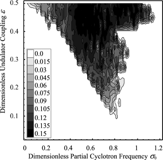
Figure 7: Map of the major Lyapunov exponent.

(6) by virtue of the first relation in (10), one can infer that the condition of non-commutative integrability holds for the system under investigation (for details see (Kozlov, 1998, p. 190)). It then follows that we can apply the Nekhoroshev theorem to find the dimensions of invariant tori (the loci of the electrons’ trajectories), which foliate the system’s phase space, Nekhoroshev (1972).

Figure 8: Projections of electron trajectories in $xy$-plane. (a) $V_{x}=-0.1c$; (b) $V_{x}=0.1c$. Bounding box is of a standard waveguide size $a\times b$ = $8.6$ mm $\times$ $4.3$ mm.

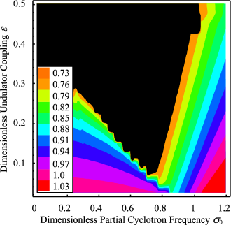
Figure 9: Contour plot of $\kappa\equiv\bar{v}_{\|}/V_{\|}$ as function of $\varepsilon$ and $\sigma_{0}$: suppression of zone of chaotic dynamics ($V_{x}=0.3V_{\|}$). The region of chaotic dynamics is given in black.

There exist four first integrals ($I$, $F_{i},i=1,2,3$) for a three dimensional nonlinear dynamical system (6), two of which ($I$ and $F_{3}$) constitute a complete set of independent first integrals in involution. Then, the dimensions of invariant tori are equal to two. Under natural projection into the system’s configuration space one can visualize such two-dimensional tori. Namely, in the reference frame, which moves with the mean velocity $\bar{v}_{\|}$ of electron (see Eqs. (III) and (A)), $\bar{\gamma}_{\|}=(1-\bar{v}^{2}_{\|}/c^{2})^{-1/2}$, its trajectory winds up a (surface diffeomorphic to) two-dimensional torus (Fig. 11). Such a regular behavior is exhibited by the dynamical system under investigation only for particular range of dimensionless parameters $\varepsilon$, $\sigma_{0}$, $V_{x}/V_{\|}$ and $V_{y}/V_{\|}$ (cf. Kozlov (1983)) as can be understood from Figs. 6, 9 and 10. When parameters change in such a way that the motion of electrons becomes chaotic, we can observe the disintegration of the corresponding invariant torus shown in Figs. 12 and 13. In Fig. 12 the trajectory of electron is drawn for a small period of time and looks like winding up a two-dimensional torus, while for a longer period of time it does not (Fig. 13).

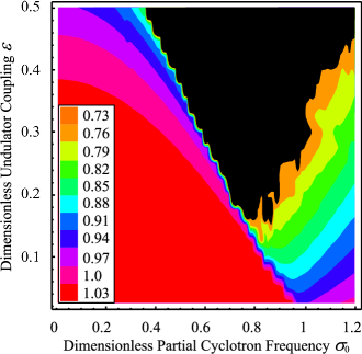
Figure 10: Contour plot of $\kappa\equiv\bar{v}_{\|}/V_{\|}$ as function of $\varepsilon$ and $\sigma_{0}$: enhancement of zone of chaotic dynamics ($V_{x}={}-0.3V_{\|}$). The region of chaotic dynamics is given in black.

Summarizing this Section, we observe that there are two regimes for pumping kinetic energy into transversal degrees of freedom of a hybrid planar FEM: the first one (advocated here as more, if not the only, efficient one for the terahertz waveband) consists in low amplitude of undulator magnetic field and the guide magnetic field as close to its magnetoresonant value as only consistent with the regular dynamics; the second regime (usually considered in the literature) would also provide the same ratio $\omega_{\perp}/(\Omega_{0}-\Omega_{\|})$ through a

Figure 11: Electron trajectory (winding of two-dimensional torus) under conditions of regular dynamics.

Figure 12: Disintegration of invariant torus for a short period of time.

high absolute value of $|\Omega_{0}-\Omega_{\|}|$ given by an off-resonant guide magnetic field $B_{\|}$ and a necessarily high value of amplitude of undulator magnetic field $B_{\perp}$. It, however, seems that values of $B_{\perp}$ in excess of $10$ kG are currently practically unattainable while guide magnetic fields of up to $50$ kG can be presently achieved.

IV Linear Amplification: Magnetostatic Resonance and Maximal Gain

As mentioned in Sec. II, analytical knowledge of electrons’ trajectories (III) in

Figure 13: Disintegration of invariant torus for a long period of time.

magnetostatic field (3) allows one to develop a gyrotron-like analytical linear theory of microwave amplification. In particular, in Ref. Goryashko et al. (2006b) such an approach was constructed for interaction of an electron beam with a mode of an arbitrary regular waveguide in a hybrid FEM. It should be noted that analytical theory of this type is valid not only far away from the magnetoresonance ($\Omega_{0}\approx\Omega_{\|}$, cf. Bratman et al. (1978)) but also in its close vicinity. Here we will apply this theory to study amplification of microwaves in a hybrid planar FEM under conditions of magnetoresonance using as an example amplification of $\mathrm{TE}_{10}$ and $\mathrm{TE}_{01}$ modes of rectangular waveguide with wide $a$ and narrow $b$ sides. Exactly these modes allow one to utilize the advantage of enhanced current of sheet electron beams (cf., for example (14)). Specifically, in each case we need to solve system (5) of ordinary differential equation with quasi-periodic coefficients. Its exact solution is achieved by application of a quasi-periodic analogue of Floquet’s theorem and, under some additional conditions, comes in the form of infinite series in undulator and cyclotron harmonics, (Haken, 1983, pp. 90-96). Under particular synchronism conditions the series may be truncated to retain solution pertinent to this very synchronism neglecting other combination ones (see Gaponov (1961); Vainshtein and Solntsev (1973)). In this case, we can write $C(z)=C_{0}\exp{(i\delta k_{z}z)}$ for the microwave amplitude ($|\delta k_{z}|\ll|k^{0}_{z}|$), where $\delta k_{z}$ is the spatial growth rate.

IV.1 Undulator synchronism

Let the undulator synchronism condition, Goryashko et al. (2006a), is fulfilled

$$\omega-k_{z}^{0}\bar{v}_{\|}\approx\Omega_{0}.$$ (11)

Using the fundamental $\mathrm{TE}_{10}$ mode ($k^{0}_{z}=[(\omega/c)^{2}-(\pi/a)^{2}]^{1/2}$) of a rectangular waveguide as an explicit demonstration example, we solve (5a) to the order $o(\varepsilon^{2})$ (retaining only summands up to the second order in $V_{\perp}/\bar{v}_{\|}$) and obtain

$$\vec{r}_{1}(\tilde{t})=r_{1}\vec{e}_{r}+r_{0}\phi_{1}\vec{e}_{\phi}+z_{1}\vec{e}_{z},$$ (12)

where

$$r_{1} = -\frac{i\pi\lambda_{w}|e|C_{0}}{4m_{e}c\,\gamma_{0}}\frac{\omega_{\perp}\Omega_{0}}{\Omega^{2}_{0}-\Omega^{2}_{\|}}\frac{\exp(i[\delta k_{z}\bar{v}_{\|}-\delta\omega]\tilde{t})}{\delta k_{z}\bar{v}_{\|}-\delta\omega}\Bigl{\{}\sin(\Omega_{\|}\tilde{t})\cos\Bigl{(}\frac{\pi}{a}\bigl{[}\bar{x}+\frac{V_{y}}{\Omega_{\|}}\bigr{]}\Bigr{)}+\Bigr{.}$$

$$\hskip 102.43008pt\Bigl{.}\frac{ia\lambda_{w}\Omega^{2}_{\|}\Omega_{0}V_{\perp}}{2\pi^{2}c^{2}(\Omega_{0}-\Omega_{\|})\bar{v}_{\|}}\sin\Bigl{(}\frac{\pi}{a}\bigl{[}\bar{x}+\frac{V_{y}}{\Omega_{\|}}\bigr{]}\Bigr{)}-\frac{\lambda_{w}^{2}\Omega_{0}^{2}V_{\perp}^{2}}{16a^{2}\Omega_{\|}^{2}\bar{v}_{\|}^{2}}\cos(\Omega_{\|}\tilde{t}-\psi)\cos\Bigl{(}\frac{\pi}{a}\bigl{[}\bar{x}+\frac{V_{y}}{\Omega_{\|}}\bigr{]}\Bigr{)}\Bigr{\}},$$

$$r_{0}\phi_{1} = -\frac{i\pi\lambda_{w}|e|C_{0}}{4m_{e}c\,\gamma_{0}}\frac{\omega_{\perp}\Omega_{0}}{\Omega^{2}_{0}-\Omega^{2}_{\|}}\frac{\exp(i[\delta k_{z}\bar{v}_{\|}-\delta\omega]\tilde{t})}{\delta k_{z}\bar{v}_{\|}-\delta\omega}\Bigl{\{}\cos(\Omega_{\|}\tilde{t})\cos\Bigl{(}\frac{\pi}{a}\bigl{[}\bar{x}+\frac{V_{y}}{\Omega_{\|}}\bigr{]}\Bigr{)}+$$

$$\hskip 88.2037pt\frac{a\lambda_{w}\Omega_{0}\Omega_{\|}(\omega+\Omega_{\|})V_{\perp}}{2\pi^{2}c^{2}(\delta k_{z}\bar{v}_{\|}-\delta\omega)\bar{v}_{\|}}\sin\Bigl{(}\frac{\pi}{a}\bigl{[}\bar{x}+\frac{V_{y}}{\Omega_{\|}}\bigr{]}\Bigr{)}+\frac{\lambda_{w}^{2}\Omega_{0}^{2}V_{\perp}^{2}}{16a^{2}\Omega_{\|}^{2}\bar{v}_{\|}^{2}}\sin(\Omega_{\|}\tilde{t}-\psi)\cos\Bigl{(}\frac{\pi}{a}\bigl{[}\bar{x}+\frac{V_{y}}{\Omega_{\|}}\bigr{]}\Bigr{)}\Bigr{\}},$$

$$z_{1} = \frac{i\pi a|e|\omega C_{0}}{2m_{e}c\,\gamma_{0}^{3}}\frac{\omega_{\perp}\Omega_{\|}}{\Omega^{2}_{0}-\Omega^{2}_{\|}}\frac{\exp(i[\delta k_{z}\bar{v}_{\|}-\delta\omega]\tilde{t})}{(\delta k_{z}\bar{v}_{\|}-\delta\omega)^{2}}\Bigl{\{}1-\frac{\lambda_{w}^{2}\Omega_{0}^{2}(\omega+\Omega_{\|})V_{\perp}^{2}}{16a^{2}\Omega_{\|}^{2}\bar{\gamma}^{2}_{\|}\omega\bar{v}_{\|}^{2}}\Bigr{\}}\sin\Bigl{(}\frac{\pi}{a}\bigl{[}\bar{x}+\frac{V_{y}}{\Omega_{\|}}\bigr{]}\Bigr{)},$$

and $\delta\omega=\omega-k_{z}^{0}\bar{v}_{\parallel}-\Omega_{0}$ is a small mismatch from the ideal synchronism ($\delta\omega=0$). It then follows that a major contribution to the spatial growth rate of the waveguide mode exists even for an electron beam with zero initial transverse velocity. For conciseness we will assume $V_{\perp}=0$ down to the end of this subsection. On the one hand for $V_{\perp}=0$ expressions (12) describe a well-known result (see Ganguly and Freund (1985)) that interaction between the transverse component of oscillatory motion and microwave results primarily in axial bunching, which becomes the main source of instability (if $V_{\perp}$ equals to zero then radial and azimuthal bunching is weaker because in this case $r_{1}$ and $r_{0}\phi_{1}$ are inversely proportional to the small quantity $(\delta k_{z}\bar{v}_{\|}-\delta\omega)$ while $z_{1}$ is inversely proportional to its square). On the other hand (unlike in Ganguly and Freund (1985)) we infer this from analytical expressions (12), which are valid for all regular dynamics parameters as found in Sec. III and, specifically, near the magnetoresonance. Substituting (12) in (5b), one then gets the dispersion equation for the $\mathrm{TE}_{10}$ mode.

Results of the outlined calculation in the case $V_{x}=V_{y}=0$ are as follows:

$$\delta k_{z}(\delta k_{z}-\frac{\delta\omega}{\bar{v}_{\|}})^{2}=\mp\frac{\pi|I_{0}|}{2c\bar{U}\gamma_{0}^{3}}\frac{\omega^{2}_{\perp}}{(\Omega_{0}^{2}-\Omega_{\|}^{2})^{2}}\times\left[\begin{array}[]{r@{,\quad}l@{\;}c@{;}}{\displaystyle\frac{\Omega_{\|}^{2}\omega}{abc}\sin^{2}\Bigl{(}\frac{\pi\bar{x}}{a}\Bigr{)}}&\mathrm{TE}_{10}\;\mbox{mode}&(k^{0}_{z}=[(\omega/c)^{2}-(\pi/a)^{2}]^{1/2})\\ {\displaystyle\frac{\Omega_{0}^{2}\omega}{abc}\sin^{2}\Bigl{(}\frac{\pi\bar{y}}{b}\Bigr{)}}&\mathrm{TE}_{01}\;\mbox{mode}&(k^{0}_{z}=[(\omega/c)^{2}-(\pi/b)^{2}]^{1/2})\end{array}\right.$$ (13)

where $\bar{U}=m_{e}\bar{v}_{\|}^{2}/(2|e|)$ is the non-relativistic beam voltage of constant motion. The conditions for existence of two complex conjugated roots of each of Eqs. (13) consist in positivity of their respective cubic discriminants. These yield in each case the thresholds for such instabilities to occur, Goryashko et al. (2007).

For the $\mathrm{TE}_{10}$ mode such a threshold condition reads

$$\frac{\delta\omega}{\bar{v}_{\|}}>{}-\frac{3}{2\gamma_{0}}\Bigl{(}\frac{\pi\omega|I_{0}|}{abc^{2}\bar{U}}\Bigr{)}^{1/3}\Bigl{(}\frac{\omega_{\perp}\Omega_{\parallel}}{\Omega_{0}^{2}-\Omega_{\parallel}^{2}}\Bigr{)}^{2/3}\sin^{2/3}\Bigl{(}\frac{\pi\bar{x}}{a}\Bigr{)}.$$

For the ideal synchronism ($\delta\omega=0$) the spatial growth rate of the $\mathrm{TE}_{10}$ mode is given by

$$\mathrm{Im}\,\delta k_{z}\!=\!\frac{\sqrt{3}}{2\gamma_{0}}\Bigl{(}\frac{\pi\omega|I_{0}|}{2abc^{2}\bar{U}}\Bigr{)}^{\!1/3}\!\!\Bigl{(}\frac{\omega_{\perp}\Omega_{\parallel}}{\Omega_{0}^{2}-\Omega_{\parallel}^{2}}\Bigr{)}^{\!\!2/3}\!\!\!\sin^{2/3}\!\Bigl{(}\frac{\pi\bar{x}}{a}\Bigr{)},$$ (14)

$\mathrm{Re}\,\delta k_{z}$ provides a correction to the cold propagation constant, $k^{0}_{z}$, caused by the presence of electron beam. Result (14) is similar to those found previously (cf., e.g. Freund and Ganguly (1986)) and also implies that there could exist a substantial enhancement in the (microwave) gain, $G=8.63\,\mathrm{Im}\,\delta k_{z}$, because of the presence of guide magnetic field. It is also significant that analytical expression (14) provides a close approximation of the growth rate, which is in a good agreement with the direct numerical simulations of the nonlinear self-consistent system of relativistic equations of motion and equations of excitation (2). This is mainly due to the fact that in $\Omega_{0}$ and $\Omega_{\|}$ we account for the initial electron velocity and magnitudes of magnetostatic fields not only through the definitions of $\omega_{0}$ and $\omega_{\|}$ but also via ‘renormalization’ multipliers $\kappa$ and $\sigma$ (cf. (8) and Fig. 2). More importantly, utilizing results obtained in Sec. III, we can provide an analytical estimate for the maximal attainable gain. To accomplish this task let us substitute from (9) to find

$$\frac{\omega_{\perp}\Omega_{\|}}{\Omega^{2}_{0}-\Omega^{2}_{\|}}<\frac{\Omega_{\|}}{\Omega_{0}+\Omega_{\|}}.$$ (15)

Recall that there exists two ways of having the value of magnetoresonant multiplier, $\omega_{\perp}/(\Omega_{0}-\Omega_{\|})$, close to $1$: one should either work far from the magnetoresonance (and provide for a strong undulator amplitude $B_{\perp}$) or, as advocated at the end of Sec. III, operate near the magnetoresonance $\Omega_{0}\approx\Omega_{\|}$ with a moderate undulator amplitude (see also Fig. 5). From the inspection of the right hand side of (15), we observe that its value is about $1/2$ around the magnetoresonance. This provides another reason for preferring a hybrid planar FEM operation regime slightly above the magnetoresonance in order to ensure the regular dynamics of electron motion as detailed in Sec. III (see also Figs. 2, 3 and 6). We, therefore, find for the upper limit on the maximal (near) magnetoresonant gain of a hybrid planar FEM under conditions of ideal undulator synchronism ($\delta\omega=0$) and $V_{\perp}=0$

$$G_{\mathrm{max}}^{\mathrm{res}}\approx\frac{3.7}{\gamma_{0}}\Bigl{(}\frac{\pi\omega|I_{0}|}{abc^{2}\bar{U}}\Bigr{)}^{1/3}\!\sin^{2/3}\Bigl{(}\frac{\pi\bar{x}}{a}\Bigr{)}.$$ (16)

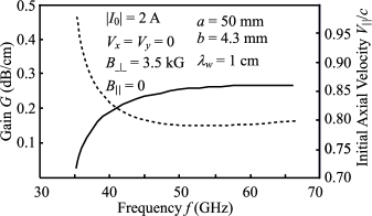
Figure 14: In the top figure results of analytical calculations of the maximal resonant gain (solid line) and initial axial velocity of the beam (dashed line) for the fundamental $\mathrm{TE}_{10}$ mode are presented. In the bottom figure we show the gain (solid line) and initial axial beam velocity (dashed line) at $B_{\|}=0$ for the $\mathrm{TE}_{01}$ mode. All quantities are shown as functions of amplified frequency.

The same conditions of regular dynamics lead to an important result that around the magnetoresonance the maximal gain is independent of $B_{\perp}$ (although entering $\bar{v}_{\|}$ in $\bar{U}$ through $\kappa$, it cancels out completely by virtue of synchronism condition ($\bar{v}_{\|}=\omega/(k_{z}^{0}(\omega)+2\pi/\lambda_{w})$); as a function of frequency, $G_{\mathrm{max}}^{\mathrm{res}}\sim(k^{0}_{z}+2\pi/\lambda_{w})^{2/3}\bar{\gamma}^{-1}_{\|}\omega^{-1/3}$.

Under the assumption of undulator synchronism in the limit $B_{\|}=0$ ($\sigma=0$ and $\kappa\approx 1-3\varepsilon^{2}/4$) an electron beam without initial transverse velocity does not interact with the $\mathrm{TE}_{m0}$ modes of a rectangular waveguide. Then the $\mathrm{TE}_{01}$ mode turns out to be the lowest one amplified by such an electron beam, and the bottom line of Eqs. (13) can be used to estimate analytically the gain of a planar FEM amplifier without the guide magnetic field (cf. Cheng et al. (1996))

$$G|_{B_{\|}=0}=\frac{5.93}{\gamma_{0}}\Bigl{(}\frac{\pi\omega|I_{0}|}{abc^{2}\bar{U}}\Bigr{)}^{1/3}\Bigl{(}\frac{\omega_{\perp}}{\Omega_{0}}\Bigr{)}^{2/3}\!\sin^{2/3}\Bigl{(}\frac{\pi\bar{y}}{b}\Bigr{)}.$$ (17)

Although, it should be noted that magnetoresonant gain ($\Omega_{0}\approx\Omega_{\|}$ and $\omega_{\perp}/(\Omega_{0}-\Omega_{\|})\approx 1$) calculated using the bottom line of Eqs. (13) is always greater than that one given by Eq. (17).

Another important characteristic of an amplifier is its tunability. In the case of undulator synchronism the frequency tuning of an FEM amplifier is achieved by changing initial axial velocity, $V_{\parallel}$, of the electron beam and turns out to be limited only by the requirement of single-mode operation regime. In Fig. 14 for the fundamental $\mathrm{TE}_{10}$ mode one can see that the maximal resonant gain depends weakly on the frequency in the operating range. To provide the single-mode operation regime and interaction only with the forward wave, the frequencies are chosen to range from $18$ GHz to $32$ GHz in this case. Results of gain calculations for interaction with the $\mathrm{TE}_{01}$ mode are also shown in Fig. 14. The initial axial velocity must also change with the frequency ($\bar{v}_{\|}=\omega/(k_{z}^{0}(\omega)+2\pi/\lambda_{w})$) as shown in the both parts of Fig. 14 to maintain the ideal undulator synchronism (in the top figure for calculation of $V_{\|}$ from a given $\bar{v}_{\|}$ we choose $\kappa=0.8$, see Fig. 6; in the bottom figure to obtain $V_{\|}$ from a given $\bar{v}_{\|}$ one needs to solve the equation $\bar{v}_{\|}=\kappa(V_{\|})V_{\|}$, see (8) and note that in this case $\sigma=0$, $V_{x}=V_{y}=0$).

IV.2 Hybrid synchronism

Under the condition of hybrid (undulator-cyclotron) synchronism, Goryashko et al. (2006a),

$$\omega-k_{z}^{0}\bar{v}_{\|}\approx\Omega_{0}+\Omega_{\|},$$ (18)

we again can solve equation (5a) to the order $o(\varepsilon^{2})$ retaining only summands up to the second order in $V_{\perp}/\bar{v}_{\|}$ and those which contain the square of the small quantity $(\delta k_{z}\bar{v}_{\|}-\delta\omega)$ in the denominators. The result for the fundamental $\mathrm{TE}_{10}$ mode has again form (12) but now with

$$r_{1} = 0,\quad r_{0}\phi_{1}\,\,=\,\,-\frac{\lambda^{3}_{w}|e|\Omega_{0}^{3}C_{0}\gamma^{2}_{\|}V_{\perp}^{2}}{32\pi m_{e}c^{3}\gamma_{0}(1+\bar{v}_{\|}^{2}\gamma_{\|}^{2}/c^{2})\bar{v}^{2}_{\|}}\frac{\omega_{\perp}}{\Omega_{0}-\Omega_{\|}}\frac{\exp(i\{[\delta k_{z}\bar{v}_{\|}-\delta\omega]\tilde{t}-\psi\})}{(\delta k_{z}\bar{v}_{\|}-\delta\omega)^{2}}\times$$

$$\hskip 202.01474pt\Bigl{\{}\frac{\kappa+3\sigma}{\kappa+\sigma}+\frac{k_{z}^{0}\lambda_{w}\kappa}{2\pi(\kappa+\sigma)}-\frac{\bar{v}_{\|}^{2}\gamma_{0}^{2}\kappa}{4c^{2}(\kappa-\sigma)}\Bigr{\}}\cos\Bigl{(}\frac{\pi}{a}\bigl{[}\bar{x}+\frac{V_{y}}{\Omega_{\|}}\bigr{]}\Bigr{)},$$

$$z_{1} = \frac{\pi\lambda_{w}|e|\Omega_{0}C_{0}V_{\perp}}{8m_{e}c\gamma_{0}(1+\bar{v}_{\|}^{2}\gamma^{2}_{\|}/c^{2})\bar{v}_{\|}}\frac{\omega_{\perp}}{\Omega_{0}-\Omega_{\|}}\frac{\exp(i\{[\delta k_{z}\bar{v}_{\|}-\delta\omega]\tilde{t}-\psi\})}{(\delta k_{z}\bar{v}_{\|}-\delta\omega)^{2}}\times$$

$$\Bigl{\{}1+\frac{k_{z}^{0}\lambda_{w}\kappa}{2\pi(\kappa+\sigma)}+\frac{\bar{v}_{\|}^{2}\gamma_{0}^{2}}{4c^{2}}\Bigl{[}\frac{\kappa^{3}-2\kappa^{2}\sigma-4\kappa\sigma^{2}+2\sigma^{3}}{\kappa(\kappa-\sigma)(\kappa+2\sigma)}-\frac{2\gamma_{\|}^{2}(\kappa^{3}+6\kappa^{2}\sigma+8\kappa\sigma^{2}-\sigma^{3})}{\gamma_{0}^{2}\kappa(\kappa+\sigma)(\kappa+2\sigma)}\Bigl{]}\Bigr{\}}\cos\Bigl{(}\frac{\pi}{a}\bigl{[}\bar{x}+\frac{V_{y}}{\Omega_{\|}}\bigr{]}\Bigr{)},$$

and $\gamma_{\|}=(1-V_{\|}^{2}/c^{2})^{-1/2}$. It then follows that the bunching mechanism is substantially axially-azimuthal, which is in contrast with the undulator synchronism where it is predominantly axial. In the non-relativistic limit the azimuthal mechanism does not contribute to the bunching being a manifestation of dependence of cyclotron frequency on the Lorentz factor (cf. Gaponov (1961)). Substituting the obtained result in (12) and then in (5b), one again gets the dispersion equation for $\mathrm{TE}_{10}$ mode under the hybrid synchronism condition.

In this manner, we obtain

$$\delta k_{z}(\delta k_{z}-\frac{\delta\omega}{\bar{v}_{\|}})^{2}=\mp\frac{\pi^{2}|I_{0}|}{8c\bar{U}\gamma_{0}(1+\bar{v}_{\|}^{2}\gamma_{\|}^{2}/c^{2})}\frac{\omega^{2}_{\perp}}{(\Omega_{0}^{2}-\Omega_{\|}^{2})^{2}}\times\left[\begin{array}[]{r@{,\quad}l@{;}}{\displaystyle\frac{\pi V^{2}_{\perp}\omega}{a^{3}b\,c}\,Q^{\mathrm{TE}}_{10}\,\cos^{2}\Bigl{(}\frac{\pi}{a}[\bar{x}+\frac{V_{y}}{\Omega_{\|}}]\Bigr{)}}&\mathrm{TE}_{10}\;\mbox{mode}\\ {\displaystyle\frac{V^{2}_{\perp}\Omega^{2}_{0}}{ab^{4}\Omega^{2}_{\|}}\,Q^{\mathrm{TE}}_{01}\cos^{2}\Bigl{(}\frac{\pi}{b}[\bar{y}-\frac{V_{x}}{\Omega_{\|}}]\Bigr{)}}&\mathrm{TE}_{01}\;\mbox{mode}\end{array}\right.$$ (20)

which are expansions to the second order in $V_{\perp}/\bar{v}_{\|}$ of the bulky analytical totally relativistic dispersion equations. Here the analytically exact expressions for the relativistic factors read

$$Q^{\mathrm{TE}}_{10} = 1-\frac{\bar{v}_{\|}^{2}\gamma_{\|}^{2}}{c^{2}}\Bigr{\{}\frac{8\pi\sigma}{k_{z}^{0}\lambda_{w}\kappa}\Bigr{[}1-\frac{\Omega_{0}(\kappa-\sigma)}{2\omega\kappa}\Bigr{]}+\frac{\Omega_{0}}{2\omega}\Bigr{[}\frac{(\kappa+\sigma)(\kappa^{2}+\kappa\sigma-\sigma^{2})}{\kappa^{2}(\kappa+2\sigma)}-$$

$$\hphantom{11{}-}\frac{\gamma_{0}^{2}(\kappa+\sigma)(\kappa^{3}-2\kappa^{2}\sigma-4\kappa\sigma^{2}+2\sigma^{3})}{2\gamma_{\|}^{2}(\kappa-\sigma)\kappa^{2}(\kappa+2\sigma)}\Bigr{]}\Bigr{\}}+\frac{\pi\bar{v}_{\|}^{4}\gamma_{0}^{2}\Omega_{0}(\kappa+\sigma)\sigma}{c^{4}k^{0}_{z}\lambda_{w}\omega(\kappa-\sigma)\kappa},$$

$$Q^{\mathrm{TE}}_{01} = 1-\frac{\bar{v}_{\|}k_{z}^{0}b\kappa\sigma}{2c(\kappa^{2}-\sigma^{2})}-\frac{2\pi\bar{v}^{2}_{\|}\gamma_{\|}^{2}\sigma}{c^{2}k_{z}^{0}\lambda_{w}\kappa}+\frac{2\pi\bar{v}^{3}_{\|}\gamma_{0}^{2}b\sigma^{2}}{c^{3}\lambda_{w}(\kappa^{2}-\sigma^{2})}-\frac{2\pi^{2}\bar{v}^{5}_{\|}\gamma_{0}^{4}b\sigma^{3}}{c^{5}k_{z}^{0}\lambda_{w}^{2}\kappa(\kappa^{2}-\sigma^{2})}.$$

Note that $k^{0}_{z}=[(\omega/c)^{2}-(\pi/a)^{2}]^{1/2}$ for the $\mathrm{TE}_{10}$ mode and $k^{0}_{z}=[(\omega/c)^{2}-(\pi/b)^{2}]^{1/2}$ for the $\mathrm{TE}_{01}$ mode, respectively.

In the non-relativistic limit (substituting $Q^{\mathrm{TE}}_{10}=1$ and keeping only the top line of expression (20) with $\gamma_{0}=\gamma_{\|}=1$ and $\bar{v}_{\|}/c\ll 1$) the obtained dispersion equation for the fundamental $\mathrm{TE}_{10}$ mode is similar to that one known in the literature (Grossman et al., 1983, Eq. (18)). However, even in this limit, not only the use of Eq. (20) is justified by our procedures for all parameter values compatible with the regular dynamics (i.e. near the magnetoresonance) but it also provides a good quantitative agreement with the direct numerical simulations of self-consistent nonlinear system (2) because of the ‘renormalization’ multipliers $\kappa$ and $\sigma$ (e.g. if one takes $\kappa$ to be equal to $1$ then $1+\bar{v}^{2}_{\|}\gamma^{2}_{\|}/c^{2}\equiv\gamma^{2}_{\|})$. It also features analytically calculated dependence of the right hand side of dispersion equation on the entrance position $\bar{x}$ of electrons (the factor $\cos^{2}(\pi[\bar{x}+V_{y}/\Omega_{\|}]/a)$). Thus, one can observe that there exist two equivalent optimal entrance position of electrons, e.g. for $|V_{y}|/\Omega_{\|}<a$ the planes $\bar{x}=-V_{y}/\Omega_{\|}$ (for $V_{y}<0$) and $\bar{x}=a-V_{y}/\Omega_{\|}$ (for $V_{y}>0$), placed near the maxima of gradient of the microwave electric field (since the electrons should not touch the waveguide walls the optimal entrance positions are not always possible). This, in principle, allows one to double the electron current by using two electron beams (with the same $x$-components and equal in value but opposite in direction $y$-components of initial velocity) and enhance the total spatial growth rate by a quarter (while simultaneously providing for reduction of aggregate space-charge effects).

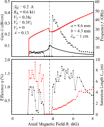
Figure 17: In the top figure solid black (gain $G$) and red (frequency $f$) lines are obtained from analytical expressions (18) and (20); the dots of respective colors are the results of direct numerical simulation of Eqs. (21) and (22). In the bottom figure black (efficiency $\eta$) and red (saturation length $L_{sat}$) dots are obtained through numerical simulation of Eqs. (21) and (22). All quantities are calculated as functions of $B_{\|}$ for the $\mathrm{TE}_{10}$ mode amplification under the hybrid synchronism. The chain lines show the position of magnetoresonance $B_{\|}^{res}\approx 3.65~{}\mbox{kG}$ (analytical calculations indicate an exponentially thin zone of chaotic dynamics for the chosen parameters).

Near the magnetoresonance, analogously to the case of undulator synchronism, there occurs a substantial reduction in the mean velocity of constant motion, $\bar{v}_{\|}$, because of kinetic energy transfer to mainly transversal oscillatory degrees of freedom. This leads to the gain growth, which is only bounded by transition to the chaotic state (see Fig. 17, $B_{\|}^{res}$ $=$ $3.65$ kG). As seen in Fig. 17 the magnetoresonance also influences essentially the dependence of ideal synchronism ($\delta\omega$) frequency on the guide magnetic field. It should be also emphasized that, as we found in Sec. III.2, the sign of $V_{x}$ has a substantial impact on the location of zones of regular and chaotic dynamics, therefore, this sign can also influence the microwave amplification. Unfortunately (because the problem involves at least six parameters), to find a set of paprameters which maximizes the right hand side of (20), we are bound to confine themselves to detailed numerical calculations. It turns out that the maximal spatial growth rate in the regular dynamics zone is attained near the magnetoresonance for $V_{x}>0$ and $V_{y}>0$, i.e. suppression of dynamical chaos near the magnetoresonance (achieved by a positive $V_{x}$, cf. Fig. 8) may allow one to enhance the spatial growth rate.

For completeness, we also provide the result of calculations for the $\mathrm{TE}_{01}$ mode given by the bottom line of Eq. (20), although to implement such an interaction in a single-mode regime one needs to take additional efforts for an efficient mode selection (see, e.g., Agafonov et al. (1998)).

V Nonlinear Simulations of Microwave Amplification

For numerical simulations of nonlinear regime of amplification it is advantageous to rewrite equations of motion (2a) taking as independent variables the coordinate $z$ and time of entrance of electrons to the interaction region $t_{e}$ (the time of arrival $t=t(z,t_{e})$ of electrons, which entered the interaction region at the time $t_{e}$, to the cross-section $z$ becomes a dependent variable) in the form

$$\begin{split}\frac{d\vec{p}}{dz}&=e\Bigl{(}\vec{E}+\bigl{[}\frac{\vec{p}}{m_{e}c\gamma}\times(\vec{B}_{p}+\vec{B})\bigr{]}\Bigr{)}\frac{dt}{dz},\\ \frac{dt}{dz}&=\frac{m_{e}\gamma}{p_{z}},\quad\frac{d\vec{r}_{\perp}}{dz}=\frac{\vec{p}_{\perp}}{p_{z}},\end{split}$$ (21)

where $\vec{E}(\vec{r}_{\perp},z,t)$, $\vec{B}(\vec{r}_{\perp},z,t)$ and $\vec{B}_{p}(\vec{r}_{\perp},z)$ are given by (1) and (3), respectively; $\vec{r}_{\perp}=(x,y)$; it is also more convenient for numerical calculations to introduce the momentum of an electron $\vec{p}=m_{e}\vec{v}\gamma$ instead of its velocity ($\vec{p}_{\perp}=(p_{x},p_{y})$, $\gamma=[1+\vec{p}\,{}^{2}/(m_{e}^{2}c^{2})]^{1/2}$). The initial conditions then are $x(z\!\!=\!\!0,t_{e})=\bar{x}$, $y(z\!\!=\!\!0,t_{e})=\bar{y}$, $t(z\!\!=\!\!0,t_{e})=t_{e}$ and $\vec{p}\,(z\!\!=\!\!0,t_{e})=m_{e}(V_{x},V_{y},V_{\|})\gamma_{0}$. Similarly, using the charge conservation law and the fact that in the stationary regime electrons, which enter the interaction region at the time $t_{e}$ separated by an integral multiple of the period of the amplified microwave, go along identical trajectories, we can write the equations of excitation (2b) for a thin electron beam as follows (Kuraev, 1971, p. 31):

$$\frac{dC}{dz}=\frac{|I_{0}|}{4\pi P_{0}}\int\limits_{0}^{2\pi}p^{-1}_{z}(\vec{p}\cdot\vec{E}^{0}(\vec{r},t))^{*}\,d(\omega t^{e})$$ (22)

Here the initial condition for the amplitude $C(z)$ reads $C(z\!\!=\!\!0)=C_{0}$. In the discrete model of electron beam we assume that over the period of the amplified microwave particles enter to the interaction region in regular time intervals $2\pi/(\omega N)$, hence, the numerical finding of solution to nonlinear self-consistent system (21) and (22) consists in the simultaneous solving of $6N+1$ first-order nonlinear ordinary differential equations.

Numerical simulations of FEM characteristics are usually concerned with those, as a rule integral, quantities, which can be directly measured experimentally (e.g. saturation power, efficiency, start current, etc.). However, a substantial advantage of numerical calculations also lies in the opportunity of detailed reconstruction of electrons dynamics and their interaction with the microwave field in an FEM. Thus, according to analytical results of Sec. IV.1, the predominant phasing mechanism on the undulator mechanism is the axial one. A numerical verification to this fact is provided in the top of Fig. 15. In the region 1, out of the uniform at entrance ($z=0$) electron beam, there occurs bunch creation under the influence of the seed microwave in its decelerating phase. The interaction of electron beam with the microwave is almost linear and the microwave power $P(z)=|C(z)|^{2}P_{0}$ grows exponentially with $2\mbox{Im}\,\delta k_{z}=0.024~{}\mbox{cm}^{-1}$. In the region 2 the electron beam is maximally bunched and efficiently amplifies the microwave (simultaneously about $0.35N$ of the beam electrons, which entered the interaction region at $z=0$ in the accelerating phase of microwave, draw the power from the microwave); the total microwave power in this region increases almost linearly. In the region 3 the electrons, which entered the interaction region at $z=0$ in the decelerating phase of microwave, do not interact with it, but the microwave power growth takes place because of interaction with approximately $0.5N$ of beam electrons that entered the interaction region at $z=0$ in the accelerating phase. In the region 4 the energy flow from the electrons, which amplify the microwave, and those that draw microwave power reaches the balance and the microwave power attains saturation. In the region 5 there occurs the second (like the region 2) consolidation of bunches at $z=230~{}\mbox{cm}$, which subsequently leads to the second maximum of microwave power at $z=280~{}\mbox{cm}$ and so on. It is also worth noting that electrons, which entered the interaction region at $z=0$ in the accelerating phase of the microwave, are weaker trapped than those entering the interaction region at $z=0$ in the decelerating phase.

Figure 15: Results of numerical calculations of electron beam bunching and microwave power amplification.

The small-amplitude fast vibrations shown in Fig. 15 are caused by the oscillations of longitudinal velocity of electrons around its mean value $\bar{v}_{\|}$ (see (III) and (A)). Note that parameter values used to produce Fig. 15 are typical for experimental designs under development, but it is not optimal in terms of efficiency of microwave amplification because of weak effective pumping of electron oscillations. As found in Sec. IV, the optimal amplification is achieved near the magnetoresonance $\Omega_{0}\approx\Omega_{\|}$. This operational regime of a hybrid planar FEM is studied in the literature analytically and numerically in comparatively less detail, mainly, inasmuch as the major attention of researches has been devoted to hybrid helix and coaxial FEM schemes. For example, in the hybrid helix scheme, one uses an annular electron beam, which adiabatic entrance is incompatible with the magnetoresonant condition Ganguly and Freund (1985) since the electrons entering the interaction region with different radial separations from the symmetry axis of the undulator magnetic field reach orbits characterized by a substantial mean velocity spread (this orbits fail to be the desired stationary helicoidal ones) and do not provide an adequate amplification of microwaves. In the planar FEM on the undulator synchronism this drawback is offset substantially because a sheet electron beam enters in the symmetry plane of the undulator magnetic field and, therefore, can efficiently amplify microwaves under the magnetoresonant condition.

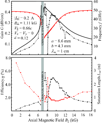
Figure 16: In the top figure solid black (gain $G$) and red (frequency $f$) lines are obtained from analytical expressions (11) and (13); the dots of respective colors are the results of direct numerical simulation of Eqs. (21) and (22). In the bottom figure black (efficiency $\eta$) and red (saturation length $L_{sat}$) dots are obtained through numerical simulation of Eqs. (21) and (22). All quantities are calculated as functions of $B_{\|}$ for the $\mathrm{TE}_{10}$ mode amplification under the undulator synchronism. The darkened area corresponds to the analytically calculated zones of chaotic dynamics around the magnetoresonance ($B_{\|}^{res}\approx 6.67~{}\mbox{kG}$).

Results of numerical calculations of various characteristics of hybrid planar FEM as functions of the guide magnetic field $B_{\|}$ are plotted in Figs. 16 and 17. One can see that the optimal amplification frequency (the frequency providing for the maximal growth rate) both for undulator and hybrid synchronisms (see (11) and (18)) depends on the guide magnetic field since the mean velocity of constant motion, $\bar{v}_{\|}$, is also a function of $B_{\|}$ at least through the ‘renormalization’ multiplier $\kappa$. Under the undulator synchronism the gain, $G$, and efficiency, $\eta$, attain their maximal values ($G\approx 0.47~{}\mbox{dB/cm}$ and $\eta\approx 5.8\%$) for the guide magnetic field ($B_{\|}\sim 7.5~{}\mbox{kG}$) greater than its magnetoresonant value. A theoretical estimate of the width of chaotic dynamics zone for the undulator synchronism gives $B_{\|}\in(6.6,7.3)~{}\mbox{kG}$ around the magnetoresonance $B_{\|}^{res}\approx 6.67~{}\mbox{kG}$. The situation is similar under the hybrid synchronism with a slight difference. The gain has a pronounced maximum $G\approx 0.37~{}\mbox{dB/cm}$ for the guide magnetic fields greater than but close to the magnetoresonant value $B_{\|}^{res}\approx 3.65~{}\mbox{kG}$, however, the maximal efficiency $\eta\approx 1.75\%$ is attained at a small finite separation ($B_{\|}\approx 4.9~{}\mbox{kG}$) from the magnetoresonance. Both cases of undulator and hybrid synchronisms show a larger efficiency of microwave amplification for guide magnetic fields greater than their respective magnetoresonant values since under such conditions a larger portion of the energy of constant longitudinal motion is transferred to the transversal oscillations of electrons.

It should be also noted that whereas the growth rate is a slow function of the amplitude of undulator magnetic field $B_{\perp}$ (or, equivalently, of $\varepsilon$), the efficiency $\eta$ grows almost linearly with it up to a certain critical value $\eta_{cr}\approx 20\%$ (e.g., $\varepsilon_{cr}\approx 0.2$ under the undulator synchronism). If $\varepsilon$ exceeds this critical value then the coherent amplification of microwave signal in the (near) magnetoresonant regime becomes impossible. In Sec. III we established that because of the Nekhoroshev theorem the motion of electrons in the magnetostatic field of hybrid planar FEM is characterized by invariant tori, overwhelming majority of which (according to the Kolmogorov-Arnold-Moser theory, see Arnold (1993)) under small perturbations of motion by a microwave signal will not be destroyed but will only be slightly deformed. Thus, interaction of electron beam with the microwave signal does not lead to a notable change of zones of chaotic and regular dynamics if this interaction is sufficiently small (cf., e.g., Figs. 6 and 16 for the undulator synchronism). However, if the interaction becomes larger of a certain critical value in the efficiency (a measure of beam-wave interaction) and, therefore, apparently, larger of a certain critical value of $\varepsilon$ then such a notable change of zones of chaotic and regular dynamics does take place, i.e. there occurs a strong widening of the domain of disintegrated invariant tori.

VI Summary and Discussions

We applied Kisunko-Vainshtein’s equations of excitation for regular waveguides to the development of self-consistent analytical linear theory of a hybrid planar FEM amplifier, which is valid not only far away but also around of the magnetoresonant value of the guide magnetic field ($\Omega_{\|}\approx\Omega_{0}$). Nonlinear numerical simulations were undertaken to clarify the validity of the linear approximation. Although, as mentioned at the beginning of this article, a number of approaches to the linear theory of a hybrid FEM has been already formulated, a new one presented here allowed us both to provide a consistent and unified analytical description of electron dynamics for all values of the guide magnetic field and, more importantly, to find an efficient characterization of the dynamical chaos present in the system. In particular, conditions of suppression of the dynamical chaos are formulated and the influence of hybrid planar FEM operational parameters on these conditions is clarified. It is also worth mentioning that the zones of suppressed beam transport found in Sakamoto et al. (1993) are in good correspondence with our (semi-)analytical calculations for the zones of dynamical chaos (cf. Fig. 1 in Sakamoto et al. (1993) and Figs. 2 and 10 of this article). This is achieved because the method of Lindshtedt employed by us to obtain test individual electron trajectories in the magnetostatic field of a hybrid planar FEM is capable of high precision in analytical calculations. It should be also mentioned that this method is sufficiently general to be applicable to describe motion of charged particles in spatially inhomogeneous static magnetic fields like, for example, that in Sakamoto et al. (1993); Cheng et al. (1996).

The origin of dynamical chaos is connected to the possibility of onset of stochastic layer around the separatrix in the system phase space (under the condition $\omega_{\perp}/\omega_{0}=[(1+V^{2}_{x}/V^{2}_{\|})^{1/2}+V_{x}/V_{\|}]/2$ motion of an electron in the undulator magnetic field takes place along the separatrix) caused by the presence of guide magnetic field, which plays the role of non-trivial perturbation capable of destruction of this separatrix (see Figs. 6, 9 and 10). The magnitude and sign of the $x$-component of initial velocity of electrons influence the position of separatrix in the phase space and allows one to adjust location of zones of regular and chaotic dynamics when the guide magnetic field is present. An approximate condition that determines the onset of chaos is given analytically and found to be in a good quantitative agreement with numerical simulations. We interpret this condition as the Chirikov resonance-overlap criterion, i.e. the chaotic behavior occurs whenever the absolute value of the difference between the normal undulator, $\Omega_{0}$, and normal cyclotron, $\Omega_{\|}$, frequencies becomes less than the coupling, $\omega_{\perp}$, induced by the undulator magnetic field. It seems also that the analytical approach developed in this paper has a strong potential for a development of analytical nonlinear in the microwave signal three-dimensional theory of a hybrid FEM.

The transfer of kinetic energy of an electron motion between longitudinal and transversal degrees of freedom is studied and it is found that the maximal fraction, $(\bar{\gamma}_{\perp}-1)/(\gamma-1)$, of the mean transversal kinetic energy is less than 30% for the case of regular dynamics. Taking into account that transversal degrees of freedom of electrons are the source of energy for the microwave field one can claim that the maximal efficiency of a hybrid planar FEM may not exceed these 30%. Using the Nehoroshev theorem we showed that motion of an individual test electron in the magnetostatic field is integrable and characterized by two-dimensional invariant tori for some range of parameters of hybrid planar FEM. As a result from the Kolmogorov-Arnold-Moser theory it then follows that for relatively moderate values of the microwave and space-charge field the electron trajectories will stay regular and amplification can still be accomplished. Through numerical simulations, we determined that the broadening of chaotic region for electron motion does not occur if the interaction between the microwave and electron beam is not too large (e.g., if such a measure of interaction intensity as the efficiency is less than 20% on the undulator synchronism).

From linearized in the microwave field equations of motion and excitation dispersion equations are derived for the undulator and hybrid synchronisms. We showed analytically that around the magnetoresonance on the undulator synchronism the gain is nearly completely independent of the amplitude of the undulator magnetic field. This circumstance is known in the literature but only as a result of numerical simulations (cf. Fig. 2 in Ginzburg et al. (2001)). Physical origin of this effect lies in the fact that the gain is a function of amplitude of transversal oscillations of electrons in the magnetostatic field of a hybrid planar FEM. Around the magnetoresonant value of guide magnetic field this amplitude, according to the chaotization criterium (9), turns out to be bounded and is independent of the amplitude of undulator magnetic field. On the undulator synchronism the obtained analytical expression for the gain provides values close to the results of nonlinear numerical simulations. Such an accuracy is achieved because of the high-precision analytical calculation of the unperturbed by the microwave proper frequencies and electron trajectories. For the hybrid synchronism we also obtained the dispersion equation but in this case the analytical expression for the gain in the zone of regular electron dynamics immediately below and above the magnetoresonant value of the guide magnetic field does not provide values close to the results of numerical calculations. We attribute this discrepancy to a greater amplitude of oscillations of the longitudinal electron velocity and, therefore, to a greater deviation (comparing to the case of the undulator synchronism) of the resultant system of ordinary differential equations from that with the strictly periodic coefficients. Solutions to such ordinary differential equations with the quasi-periodic coefficients does not follow patterns of their counterparts with the periodic coefficients especially in the vicinity of (combination) resonances between their proper frequencies. Nevertheless, we showed analytically and verified through numerical simulations that operation of a hybrid planar FEM in the (near) magnetoresonant regime is optimal in order to achieve the maximal gain and efficiency. The interaction between transversal degrees of freedom of electrons and microwave field under such conditions turns out to be maximal out of all other possible operation parameters of a hybrid planar FEM on each of the synchronisms (experimentally for a hybrid planar FEM oscillator such an operational regime was established, for example, in Bratman et al. (1996)). The major result here is that one needs not only to have a small value of $\varepsilon$ in order to maintain the relation $\bar{v}_{\|}\gg\bar{v}_{\perp}$ ($\bar{v}_{\perp}$ is the mean transversal velocity) but also to hold the ratio $\varepsilon/|\kappa-\sigma|\equiv\omega_{\perp}/|\Omega_{0}-\Omega_{\|}|$ as close to the unity as possible thus providing for the maximal gain and efficiency.

Here we have not considered any specific arrangements usually applied for a smooth (at best adiabatic) entrance of an electron beam to the interaction region, which lead us to neglect of the velocity and position spread of electrons at the entrance to the interaction region. The developed techniques are fully capable of treating these effects but taking them into account in the framework of the current consideration would make our treatment overcomplicated and hide behind the technicalities the physics underlying the nature of dynamical chaos in a hybrid planar FEM. This paper also does not deal with the influence of the space-charge field on operational characteristics of a hybrid planar FEM. It is necessary to notice that space-charge field strongly decreases the efficiency of interaction between an electron beam and amplified microwave if the regime of operation is positioned far away from the magnetoresonance. However, there are strong indications that not only the amplification of a microwave signal by an electron beam becomes maximal around the magnetoresonance but also the defocusing influence of the present space-charge field turns out to be minimal. A detailed investigation of the influence of potential (irrotational) and rotational parts of the space-charge field on the operation of a weakly-relativistic hybrid FEM will be published elsewhere.

*

Appendix A Velocity to the Order $o(\varepsilon^{3})$

Here we present terms of the order $\mathcal{O}(\varepsilon^{2})$, which should be added componentwise to expressions (III) to obtain solutions to the electron velocities valid to the order $o(\varepsilon^{3})$. These additional contributions read

$$\dot{x}_{0}^{add}(\tilde{t}) = -2V_{\perp}\frac{\omega_{\perp}^{2}\Omega_{0}^{3}\Omega_{\|}}{(\Omega_{0}^{2}-\Omega_{\|}^{2})^{3}}\Bigl{[}\sin(\Omega_{0}\tilde{t})\sin\psi-\frac{3\Omega_{0}^{4}+6\Omega_{0}^{2}\Omega_{\|}^{2}-\Omega_{\|}^{4}}{16\Omega_{0}^{3}\Omega_{\|}}\cos(\Omega_{\|}\tilde{t}-\psi)-\frac{\Omega_{0}^{2}-5\Omega_{\|}^{2}}{16\Omega_{0}\Omega_{\|}}\cos(\Omega_{\|}\tilde{t}+\psi)+$$

$$\frac{(\Omega_{0}-\Omega_{\|})^{3}(2\Omega_{0}+\Omega_{\|})^{2}}{32\Omega_{0}^{4}\Omega_{\|}}\cos([2\Omega_{0}+\Omega_{\|}]\tilde{t}-\psi)+\frac{(\Omega_{0}+\Omega_{\|})^{3}(2\Omega_{0}-\Omega_{\|})^{2}}{32\Omega_{0}^{4}\Omega_{\|}}\cos([2\Omega_{0}-\Omega_{\|}]\tilde{t}+\psi)\Bigr{]},$$

$$\dot{y}_{0}^{add}(\tilde{t}) = -2V_{\perp}\frac{\omega_{\perp}^{2}\Omega_{0}^{2}\Omega_{\|}^{2}}{(\Omega_{0}^{2}-\Omega_{\|}^{2})^{3}}\Bigl{[}\cos(\Omega_{0}\tilde{t})\sin\psi+\frac{3\Omega_{0}^{4}+6\Omega_{0}^{2}\Omega_{\|}^{2}-\Omega_{\|}^{4}}{16\Omega_{0}^{2}\Omega_{\|}^{2}}\sin(\Omega_{\|}\tilde{t}-\psi)+\frac{\Omega_{0}^{2}-5\Omega_{\|}^{2}}{16\Omega_{\|}^{2}}\sin(\Omega_{\|}\tilde{t}+\psi)-$$

$$\frac{(\Omega_{0}+\Omega_{\|})^{3}(2\Omega_{0}-\Omega_{\|})}{32\Omega_{0}^{3}\Omega_{\|}}\sin([2\Omega_{0}-\Omega_{\|}]\tilde{t}+\psi)-\frac{(\Omega_{0}-\Omega_{\|})^{3}(2\Omega_{0}+\Omega_{\|})}{32\Omega_{0}^{3}\Omega_{\|}}\sin([2\Omega_{0}+\Omega_{\|}]\tilde{t}-\psi)+\frac{\Omega_{0}^{4}-\Omega_{\|}^{4}}{8\Omega_{0}^{2}\Omega_{\|}^{2}}\sin\psi\Bigr{]},$$

$$\dot{z}_{0}^{add}(\tilde{t}) = -\frac{\omega_{\perp}^{2}\bar{v}_{\|}^{6}\Omega_{0}\lambda_{w}}{32\pi V_{\|}^{6}(\Omega_{0}^{2}-\Omega_{\|}^{2})}\Bigl{[}\Bigl{\{}4-2\frac{V_{\perp}^{2}(\Omega_{0}^{2}+\Omega_{\|}^{2})}{\bar{v}_{\|}^{2}(\Omega_{0}^{2}-\Omega_{\|}^{2})}\Bigr{\}}\cos(2\Omega_{0}\tilde{t})+4\frac{V_{\perp}^{2}\Omega_{0}^{2}}{\bar{v}_{\|}^{2}(\Omega_{0}^{2}-\Omega_{\|}^{2})}\cos(2\Omega_{\|}\tilde{t}-2\psi)-$$

$$8\frac{\Omega_{0}^{3}(\Omega_{0}+\Omega_{\|})}{(\Omega_{0}^{2}-\Omega_{\|}^{2})^{2}}\Bigl{\{}\Bigl{(}1-\frac{\Omega_{\|}^{2}}{\Omega_{0}^{2}}+\frac{V_{\perp}^{2}\Omega_{\|}}{\bar{v}_{\|}^{2}\Omega_{0}}\Bigr{)}\cos([\Omega_{0}-\Omega_{\|}]\tilde{t})-\frac{V_{\perp}^{2}\Omega_{\|}}{\bar{v}_{\|}^{2}\Omega_{0}}\cos([\Omega_{0}-\Omega_{\|}]\tilde{t}+2\psi)\Bigr{\}}-$$

$$8\frac{\Omega_{0}^{3}(\Omega_{0}-\Omega_{\|})}{(\Omega_{0}^{2}-\Omega_{\|}^{2})^{2}}\Bigl{\{}\Bigl{(}1-\frac{\Omega_{\|}^{2}}{\Omega_{0}^{2}}-\frac{V_{\perp}^{2}\Omega_{\|}}{\bar{v}_{\|}^{2}\Omega_{0}}\Bigr{)}\cos([\Omega_{0}+\Omega_{\|}]\tilde{t})+\frac{V_{\perp}^{2}\Omega_{\|}}{\bar{v}_{\|}^{2}\Omega_{0}}\cos([\Omega_{0}+\Omega_{\|}]\tilde{t}-2\psi)\Bigr{\}}-$$

$$\frac{V_{\perp}^{2}}{\bar{v}_{\|}^{2}}\Bigl{\{}\frac{\Omega_{0}(\Omega_{0}+\Omega_{\|})}{(\Omega_{0}-\Omega_{\|})^{2}}\cos(2[\Omega_{0}-\Omega_{\|}]\tilde{t}+2\psi)+\frac{\Omega_{0}(\Omega_{0}-\Omega_{\|})}{(\Omega_{0}+\Omega_{\|})^{2}}\cos(2[\Omega_{0}+\Omega_{\|}]\tilde{t}-2\psi)\Bigr{\}}\Bigr{]}.$$

References

- Sprangle and Granatstein (1978) P. Sprangle and V. L. Granatstein, Phys. Rev. A 17, 1792 (1978).
- Parker et al. (1982) R. K. Parker, R. H. Jackson, S. H. Gold, H. P. Freund, V. L. Granatstein, P. C. Efthimion, M. Herndon, and A. K. Kinkead, Phys. Rev. Lett. 48, 238 (1982).
- Andruszkow et al. (2000) J. Andruszkow, B. Aune, V. Ayvazyan, and et al., Phys. Rev. Lett. 85, 3825 (2000).
- Agafonov et al. (1998) M. A. Agafonov, A. V. Arzhannikov, N. S. Ginzburg, V. G. Ivannenko, P. V. Kalinin, S. A. Kuznetsov, N. Y. Peskov, and S. L. Sinitsky, IEEE Trans. Plasma Sci. 26, 531 (1998).
- Louisell et al. (1979) W. H. Louisell, J. F. Lam, D. A. Copeland, and W. B. Colson, Phys. Rev. A 19, 288 (1979).
- Freund et al. (1981) H. P. Freund, P. Sprangle, D. Dillenburg, E. H. da Jornada, B. Liberman, and R. S. Schneider, Phys. Rev. A 24, 1965 (1981).
- Kokhmanskii and Kulish (1984) S. S. Kokhmanskii and V. V. Kulish, Acta Phys. Polon. A 66, 713 (1984).
- Masud et al. (1986) J. Masud, T. C. Marshall, S. P. Schlesinger, and F. G. Yee, Phys. Rev. Lett. 56, 1567 (1986).
- Ginzburg and Novozhilova (1986) N. S. Ginzburg and Y. V. Novozhilova, Sov. Phys. Tech. Phys. 31, 1017 (1986).
- Conde and Bekefi (1991) M. E. Conde and G. Bekefi, Phys. Rev. Lett. 67, 3082 (1991).
- Viktorov et al. (1991) Y. B. Viktorov, A. B. Draganov, A. K. Kaminsky, N. Y. Kotsarenko, S. B. Rubin, V. P. Sarantsev, A. P. Sergeev, and A. A. Silivra, Zhurnal Tekhn. Fiz. 61, 133 (1991).
- Sakamoto et al. (1993) K. Sakamoto, T. Kobayashi, Y. Kishimoto, S. Kawasaki, S. Musyoki, A. Watanabe, M. Takahashi, H. Ishizuka, and M. Shiho, Phys. Rev. Lett. 70, 441 (1993).
- Bratman et al. (1996) V. L. Bratman, G. G. Denisov, N. S. Ginzburg, B. D. Kol’chugin, N. Y. Peskov, S. V. Samsonov, and A. B. Volkov, IEEE Trans. Plasma Sci. 24, 744 (1996).
- Chen and Donaldson (1990) C. Chen and R. C. Donaldson, Phys. Rev. A 42, 5041 (1990).
- Chen and Donaldson (1991) C. Chen and R. C. Donaldson, Phys. Rev. A 43, 5541 (1991).
- Freund and Antonsen (1995) H. P. Freund and T. M. Antonsen, Principles of Free-Electron Lasers (Chapman & Hall, New York, USA, 1995).
- Yefimov et al. (2004) B. P. Yefimov, K. V. Ilyenko, T. Y. Yatsenko, and V. A. Goryashko, Telecommun. Radio Engineer. 61, 243 (2004).
- Goryashko et al. (2006a) V. A. Goryashko, K. V. Ilyenko, and A. N. Opanasenko, Telecommun. Radio Engineer. 65, 991 (2006a).
- Kisunko (1949) G. V. Kisunko, Electrodynamics of hollow structures (Red Banner Millitary Academy of Communications, Leningrad, USSR, 1949), (in Russian).
- Vainshtein and Solntsev (1973) L. A. Vainshtein and V. A. Solntsev, Lectures on high-frequency electronics (Soviet Radio, Moscow, USSR, 1973), (in Russian).
- Gaponov (1961) A. V. Gaponov, Izv. Vyssh. Ucheb. Zaved. Radiofiz. 4, 547 (1961).
- Gover (1995) A. Gover, Phys. Rev. E 51, 2472 (1995).
- Cheng et al. (1996) S. Cheng, W. W. Destler, V. L. Granatstein, T. M. Antonsen, B. Levush, J. Rodgers, and Z. X. Zhang, IEEE Trans. Plasma Sci. 24, 750 (1996).
- Friedland and Hirshfield (1980) L. Friedland and J. L. Hirshfield, Phys. Rev. Lett. 44, 1456 (1980).
- Colson (1981) W. B. Colson, IEEE J. Quantum Electron. 17, 1417 (1981).
- Lieberman and Lichtenberg (1992) M. A. Lieberman and A. J. Lichtenberg, Regular and chaotic dynamics (Springer-Verlag, New York, USA, 1992).
- Linshtedt (1883) A. Linshtedt, Memoirs l’Acad. Sci. St.-Peterbourg. 31, 1 (1883).
- Blaquiere (1966) A. Blaquiere, Nonlinear system analysis (Academic Press, New York, USA, 1966).
- Rabinovich and Trubetskov (1989) M. I. Rabinovich and D. I. Trubetskov, Oscillations and waves in linear and nonlinear systems (Kluwer Academic, Dordrecht, Germany, 1989).
- Arnold (1993) V. I. Arnold, Mathematical aspects of classical and celestial mechanics (Springer-Verlag, Berlin, Germany, 1993).
- Sagdeev et al. (1988) R. Z. Sagdeev, D. A. Usikov, and G. M. Zaslavsky, Nonlinear physics : from the pendulum to turbulence and chaos (Harwood Academic, New York, USA, 1988).
- Grossman et al. (1983) A. Grossman, T. C. Marshall, and S. P. Schlesinger, Phys. Fluids 26, 337 (1983).
- Chirikov (1979) B. V. Chirikov, Phys. Rep. 52, 263 (1979).
- Kozlov (1998) V. V. Kozlov, General theory of vortices (Regular and Chaotic Dynamics, Izhevsk, Russia, 1998), (in Russian).
- Nekhoroshev (1972) N. N. Nekhoroshev, Trans. Mosc. Math. Soc. 26, 121 (1972).
- Kozlov (1983) V. V. Kozlov, Russ. Math. Surv. 38, 1 (1983).
- Goryashko et al. (2006b) V. A. Goryashko, K. V. Ilyenko, and A. N. Opanasenko, Radiofiz. Elektronika 11, 440 (2006b).
- Bratman et al. (1978) V. L. Bratman, N. S. Ginzburg, and M. I. Petelin, JETP Lett. 28, 190 (1978).
- Haken (1983) H. Haken, Advanced Synergetics (Springer-Verlag, Berlin, Germany, 1983).
- Ganguly and Freund (1985) A. K. Ganguly and H. P. Freund, Phys. Rev. A 32, 2275 (1985).
- Goryashko et al. (2007) V. Goryashko, K. Ilyenko, and A. Opanasenko, Proceedings of the Eighth IEEE International Vacuum Electronics Conference, Kitakyushu, Japan, p. 291 (2007).
- Freund and Ganguly (1986) H. P. Freund and A. K. Ganguly, Phys. Rev. A 33, 1060 (1986).
- Kuraev (1971) A. A. Kuraev, Ultrahighfrequency devices with periodic electron flows (Science and Engineering, Minsk, USSR, 1971), (in Russian).
- Ginzburg et al. (2001) N. S. Ginzburg, R. M. Rozental, N. Y. Peskov, A. V. Arzhannikov, and S. L. Sinitskii, Phys. Tech. Journal 46, 1545 (2001).