Inhomogeneous baryogenesis, cosmic antimatter, and dark matter

Abstract

A model of inhomogeneous baryogenesis based on the Affleck and Dine mechanism is described. A simple coupling of the scalar baryon field to the inflaton allows for formation of astronomically significant bubbles with a large baryon (or antibaryon) asymmetry. During the farther evolution these domains form compact stellar-like objects, or lower density clouds, or primordial black holes of different size. According to the scenario, such high baryonic number objects occupy relatively small fraction of space but despite that they may significantly contribute to the cosmological mass density. For some values of parameters the model allows the possibility the whole dark matter in the universe to be baryonic. Furthermore, the model allows the existence of the antibaryonic B-bubbles, i.e. a significant fraction of the mass density in the universe can be in the form of the compact antimatter objects (e.g. anti-stars).

1 Introduction

Though the universe in our neighbourhood looks as 100% baryonic, the observations do not exclude subdominant but astronomically large domains and objects of antimatter. For a recent analysis and literature see e.g. ref. [1, 2]. The standard mechanism of baryogenesis [3] predicts baryon asymmetry expressed as the ratio of baryon-to-photon number densities:

$$\beta=n_{B}/n_{\gamma}$$ (1)

to be constant both in space and, after baryogenesis is over, also in time, however, more complicated models can lead to not so dull pattern. The outcome of the baryogenesis scenario is closely related to the mechanism of CP-violation realized in cosmology. For a review of the latter see ref. [4]. If CP is broken spontaneously [5], the universe would be charge symmetric with equal weight of baryonic and antibaryonic domains so that the average value of $\beta$ over whole universe would be zero [6, 7]. However, in the standard cosmology the domain size would be very small by astronomical standards and some exponential (inflationary) expansion is necessary to avoid immediate problems [8, 9]. Another cosmological problem of domain walls with huge energy density inside our horizon [6] can be solved either by non-restoration of CP invariance at high temperature [10, 11], but in this case antimatter domains would not be created, or by a possible mechanism of wall destruction [12, 13]. However, even if these problems are resolved, it can be shown that baryo-symmetric cosmology demands the domain size above (a few) Gpc. Otherwise too intensive gamma ray background would be created by the annihilation on the domain boundaries  [14].

If in addition to spontaneous CP-violation there exists an explicit one, the universe would be baryo-asymmetric and, if the magnitude of spontaneous CP breaking happened to be larger than the explicit one, there could exist subdominant antimatter domains  [12, 13, 15].

Here we explore another mechanism of inhomogeneous baryogenesis suggested in ref. [16]. This mechanism is based on the Affleck and Dine [17] idea that in supersymmetric theories a complex scalar field $\chi$ with non-zero baryonic number may be displaced far from the origin, $\chi=0$, along flat directions of the potential $U(\chi)$. Such flat directions are generic features of supersymmetric models. Inflationary stage is especially favorable for such a travel along the flat directions due to the infrared instability of massless or light, $m^{2}_{\chi}\ll H^{2}$, fields in De Sitter space-time. According to the results of ref. [18, 19, 20] (see however, ref. [21]), vacuum expectation value of massless scalar field rises as:

$$\langle\chi^{2}\rangle=H^{3}t/4\pi^{2}\;.$$ (2)

Inflation not only drives $\chi$ away from the origin but also allows for formation of the exponentially big domains with a large value of $\chi$.

After the Hubble parameter, $H$, dropped below $m_{\chi}$, the scalar baryon (AD-field) $\chi$ would evolve down to $\chi=0$ transforming the accumulated baryonic charge into quarks by $B$-conserving decays. Typically such scenario leads to a large baryon asymmetry, $\beta\sim 1$ and theoretical efforts should be taken to diminish it down to the observed value $\beta\approx 5\cdot 10^{-10}$.

The modification of this mechanism, according to ref. [16], was an introduction of the quadratic coupling of $\chi$ to the inflaton field $\Phi$ in the following renormalizable form, $\lambda_{1}|\chi|^{2}(\Phi^{2}+\tilde{\mu}\Phi)$, where $\tilde{\mu}$ is a constant parameter with dimension of mass. This term can be rewritten as:

$$U_{int}(\chi,\Phi)=\lambda_{1}|\chi|^{2}\left(\Phi-\Phi_{1}\right)^{2}$$ (3)

by redefinition of the mass term of $\chi$.

When the inflaton field evolves down to zero, it passes through $\Phi=\Phi_{1}$ and at that moment the window to flat direction in $\chi$ potential would be open but only for a rather short period of time. Correspondingly, the probability for $\chi$ to evolve away from the origin would be small and baryogenesis resulting in high $\beta$ could proceed only in a minor fraction of space. So we should expect that in the bulk of space the usual homogeneous baryogenesis took place, and compact B-bubbles, with very high baryonic number density could be created over this background. Despite their small size, B-bubbles might contribute significant amount into the total cosmological mass density and even make all dark matter of the universe. They would either form compact stellar-like objects, or high density clouds, or primordial black holes (BH). In the simplest version of the model there should be an equal number of baryonic and antibaryonic B-bubbles. So cosmology would be almost baryo-symmetric but the bounds derived in ref. [14] are not applicable here because of compactness of the bubbles. An interesting feature of this scenario is that dark matter (DM) can be made from the usual particles, baryons and antibaryons in the form of evolved stellar type objects or primordial black holes.

The paper is organized as follows. In the Sec. 2 we give a detailed description of the model and it’s parameter space. The B-bubble evolution and the generation of the baryon asymmetry are discussed in Sec. 3. The next section, Sec. 4, gives a detailed description of the development of quantum fluctuations of the Affleck and Dine field and the distribution of B-bubbles over the length and mass. In Sec. 5 the fate of B-bubbles during different cosmological epochs is considered. In Sec.6 the observational bounds on the dark matter in the form of primordial black holes (PBH) and the amount af antimatter in the compact stellar objects are presented. Our conclusions are hosted in the Sec. 7.

2 The model and the parameter space

First we will study qualitatively the evolution of $\chi$ and formation of the bubbles with a large value of this field. Though the model and results are similar to those of ref. [16], here we discuss a somewhat simpler scenario.

Let us consider a toy model which can lead to the features described in the Introduction. We assume that the evolution of the inflaton field is governed by the usual potential:

$$U_{\Phi}(\Phi)=m_{\Phi}^{2}\Phi^{2}/2+\lambda_{\Phi}\Phi^{4}/4,$$ (4)

while $\chi$ “lives” in the potential

$$U_{\chi}(\chi,\Phi)=\lambda_{1}(\Phi-\Phi_{1})^{2}|\chi|^{2}+\lambda_{2}|\chi|^{4}\ln{\frac{|\chi|^{2}}{\sigma^{2}}}+m_{0}^{2}|\chi|^{2}+m_{1}^{2}\chi^{2}+m_{1}^{*2}\chi^{*2}.$$ (5)

The first term in this expression describes the interaction between the inflaton and $\chi$ fields introduced in ref. [16]. We assume that $\lambda_{1}$ and $|\chi|$ are sufficiently small, and so this term has negligible impact on the inflaton evolution. The second term is the Coleman-Weinberg potential [22] obtained by summation of one loop corrections to the quartic potential, $\lambda_{2}|\chi|^{4}$. The last two mass terms are not invariant with respect to the phase rotation:

$$\chi\rightarrow e^{i\theta}\chi$$ (6)

and thus break baryonic charge conservation (see below). If $m_{0}^{2}<2|m_{1}|^{2}$, the potential created by these two terms is not bounded from below but the effective mass:

$$m_{eff}^{2}=\lambda_{1}(\Phi-\Phi_{1})^{2}+m_{0}^{2}+2|m_{1}|^{2}\cos(2\alpha+2\theta)$$ (7)

is almost always positive, except for a short time when $\Phi\approx\Phi_{1}$. Anyhow the $\lambda_{2}|\chi|^{4}\ln|\chi|^{2}$ term stabilizes the potential but its minimum shifts from $\chi^{(1)}=0$ to some non-zero $\chi$. In the above equation $\alpha$ and $\theta$ are the phases of mass, $m_{1}=|m_{1}|\exp(i\alpha)$, and of AD-field, $\chi=|\chi|\exp(i\theta)$, respectively.

It is interesting that potential (5) conserves CP despite presence of the complex mass parameters. Indeed the imaginary part of $m$ can be excluded by the redefinition $\chi\rightarrow\chi\exp(-i\alpha)$. However, a coupling of $\chi$ to fermions may destroy CP-conservation.

Classical evolution of homogeneous fields $\Phi$ and $\chi$ is determined by the equations

$$\ddot{\Phi}+3H\Phi+m_{\Phi}^{2}\Phi+\lambda_{\Phi}\Phi^{3}+2\lambda_{1}|\chi|^{2}(\Phi-\Phi_{1})=0\;,$$ (8)

$$\ddot{\chi}+3H\dot{\chi}+\lambda_{1}(\Phi-\Phi_{1})^{2}\chi+\lambda_{2}|\chi|^{2}\chi\left(2\ln\frac{|\chi|^{2}}{\sigma^{2}}+1\right)+2m^{*2}\chi^{*}=0\;,$$ (9)

which we solved numerically, but qualitative behavior of the solutions can be understood from the following simple considerations. We start from inflationary stage when the cosmological energy density is dominated by the inflaton field. We assume that the product $\lambda_{1}|\chi|^{2}$ is sufficiently small, so the $\chi$-dependent term in eq. (8) is not essential. In this regime the evolution of $\Phi$ is simply a slow roll in the corresponding potential (4) till the Hubble parameter remains large in comparison with the potential slope:

$$H^{2}=\frac{8\pi}{3m_{Pl}^{2}}\,\left(\frac{m_{\Phi}^{2}\Phi^{2}}{2}+\frac{\lambda_{\phi}\Phi^{4}}{4}\right)\gg U^{\prime\prime}(\Phi)=m_{\Phi}^{2}+3\lambda_{\Phi}\Phi^{2}\;.$$ (10)

In the course of the cosmological expansion $\Phi$ approaches the equilibrium point $\Phi=0$ and $H$ drops down so that

$$H^{2}\leq m^{2}(\Phi)=m_{\Phi}^{2}+3\lambda_{\Phi}\Phi^{2}\;.$$ (11)

Inflation stops and $\Phi$ starts to oscillate around $\Phi=0$ producing particles and heating the universe. Correspondingly, the De Sitter expansion regime with domination of the vacuum-like energy turns into the matter domination and later into the radiation domination. To be more precise the equilibrium value of $\Phi$ depends upon $\chi$. But as we will see below, $\chi$ ultimately tends to zero and during inflationary period this correction is not of much importance. If the life-time of $\chi$ is longer than the life-time of the inflaton, the impact of $\chi$ on the inflaton behavior might be essential at the (re/pre)heating.

According to our assumption and with our choice of the parameters, the impact of $\chi$ on the inflaton behavior is almost unimportant. Therefore during the qualitative discussion we consider the evolution of $\chi$ in the fixed (but still time dependent) inflaton background. However, we have not neglected corresponding term when solved the equations numerically.

At the beginning of inflation, $\Phi$ is large, $\Phi>m_{Pl}$, and the effective mass of $\chi$ (7) is also large. During this period potential (5) has only one minimum at $\chi=0$ and if $m_{eff}$, eq. (7), is large in comparison with $H$, quantum fluctuations of $\chi$ are not essential and field $\chi$ “sits” in the minimum $\chi^{(1)}=0$.

In fact the picture is more complicated. If $\lambda_{\phi}\neq 0$, then for large $\Phi$ the Hubble parameter would be larger than $m_{eff}$ and $\chi$ could quantum fluctuate away from zero climbing up the potential slope during an early inflationary stage. With decreasing $H$ field $\chi$ would return back to zero if the classical rolling down of $\chi$ is faster than the decrease of $H$.

When the amplitude of the inflaton drops down and approaches $\Phi_{1}$, the effective mass of $\chi$ decreases and the potential gets the second minimum at some $\chi^{(2)}\neq 0$. This second minimum appears and disappears when $m^{2}_{eff}$ passes down and up the value $2\lambda_{2}\sigma^{2}/e^{3/2}$. Initially the second minimum at $\chi=\chi^{(2)}$ lays above the minimum at $\chi^{(1)}=0$, and later with the diminishing difference $|\Phi-\Phi_{1}|$ it becomes the absolute minimum, but separated from the minimum at $\chi^{(1)}=0$ by a barrier. In this situation the first order phase transition by quantum tunneling from $\chi=0$ to $\chi=\chi^{(2)}$ is possible, but the transition probability is exponentially small and the process can be neglected. The transition to $\chi=\chi^{(2)}$ would be much more efficient when the barrier became low or disappeared. It is essential that the low barrier existed only for some finite time. After $\Phi$ passed $\Phi_{1}$ and traveled further to zero, the potential barrier would reappear. The behavior of $U(\chi,\Phi)$ is depicted in Fig. 1. As a result of such non-monotonic behavior of the potential, $\chi$ would be either forced back to the first minimum at $\chi=0$ or would remain beyond the barrier near $\chi=\chi^{(2)}$. The separation depends upon the amplitude which $\chi$ managed to reach to the moment of the “gate closing”. The boundary/critical value of $\chi$ is determined by the position of the maximum of $U(\chi,\Phi)$ at $\chi=\chi^{(3)}$, which separates the two minima (see Fig. 1). $\chi^{(3)}$ is the smaller solution of the equation:

$$2\lambda_{2}|\chi|^{2}\,\ln\frac{\sqrt{e}|\chi|^{2}}{\sigma^{2}}+m^{2}_{eff}=0$$ (12)

and by an order of magnitude: $\chi^{(3)}\sim m_{eff}/\sqrt{\lambda_{2}}$. An important feature of $\chi_{3}$ is that it is not constant but moves together with $\Phi$.

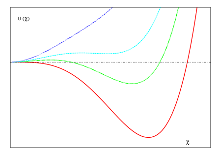
Figure 1: Qualitative behaviour of $U_{\chi}(\chi)$ for different values of $m^{2}_{eff}(t)$.

Thus we expect that for some time, when the second minimum at $\chi^{(2)}$ existed, there should be two phases with large $\chi\sim\chi^{(2)}$ and small $\chi\sim 0$. Which phase dominates is determined by the duration of the “open gate” period and the efficiency of quantum fluctuations of $\chi$. We will show in what follows (Sec. 4) that one can naturally realize the scenario when the probability of formation of large $\chi$ bubbles is sufficiently small and they would occupy a small fraction of the total volume of the universe. Still their size can be astronomically large if they were formed during inflationary stage. In other words, when $\Phi$ was close to $\Phi_{1}$, inflation lasted sufficiently long to stretch up the bubble size exponentially. In the future such bubbles would form objects (or domains) with a large value of the baryon asymmetry and we will call them B-bubbles or just BBs.

Note that the phase transition (p.t.) which we discuss here is neither first order, nor second order but something in between. It takes place when the barrier is absent and in this sense it is second order but it resulted in formation of bubbles of new phase inside the old one and, as such, it resembles the first order p.t. Note that the evolution of $\chi$ demonstrates the hysteresis behavior. Initially when $\chi$ was near zero, it remained there despite appearance of the second minimum of the potential at $\chi^{(2)}$. At a later stage when the second minimum became higher than the first one, $\chi$ remained there and rolled down to $\chi=0$ only when the minimum $\chi^{(2)}$ completely disappeared.

We assume that $m_{0}^{2}>2m_{1}^{2}$, so the local minimum of $U_{\chi}$ never disappears and classically $\chi$ should always remain zero. However, quantum fluctuations of light, $m<H$, scalars in De Sitter background allow to overcome this barrier. Roughly speaking it is possible when $\lambda_{1}(\Phi-\Phi_{1})^{2}<H^{2}$ and thus the characteristic time when the gate to the negative slope of the potential was open, lasted approximately

$$\Delta t\approx\frac{3H^{2}}{\sqrt{\lambda_{1}}U^{\prime}_{\Phi}}=\frac{2\pi\Phi_{1}(2m_{\Phi}^{2}+\lambda_{\Phi}\Phi_{1}^{2})}{\sqrt{\lambda_{1}}m_{Pl}^{2}(m_{\Phi}^{2}+\lambda_{\Phi}\Phi_{1}^{2})}\;,$$ (13)

where we used the slow roll approximation: $\dot{\Phi}\approx U^{\prime}_{\Phi}/3H$. According to eq. (2), during this time interval $\chi$ can reach the value of the order of

$$\chi^{2}\sim\frac{H^{3}\Delta t}{4\pi^{2}}\sim\sqrt{\frac{2\pi}{27\lambda_{1}}}\,\frac{\Phi_{1}^{4}}{m_{Pl}^{5}}\,\frac{(2m_{\Phi}^{2}+\lambda_{\Phi}\Phi_{1}^{2})^{5/2}}{m_{\Phi}^{2}+\lambda_{\Phi}\Phi_{1}^{2}}$$ (14)

For the chosen below parameters $\chi$ can reach the boundary value $\chi_{c}$ after which it would evolve classically down to the second minimum of $U_{\chi}$.

Since during this period $m_{1}^{2}$ was much smaller than $H^{2}$, the phase of $\chi$ equally populated the interval $[0,2\pi]$. This would allow for generation of bubbles with a large baryon asymmetry. On the other hand, if $\chi$ stays in the minimum over the phase variable i.e. at $\cos(2\alpha+2\theta)=-1$, the baryon asymmetry would be small, because no “angular momentum” can be generated in the process of the evolution of $\chi$ down to zero, despite the non-sphericity of the potential (see Sec. 3). Such a case could be realized if $\chi$ evolved to $\chi_{2}$ along the path $\alpha+\theta=\pi/2$. However, even in this case the $\chi$-state initially localized near this value of the phase, would be dispersed by quantum fluctuations over all values of the phase because the mass of the pseudogoldstone degree of freedom is much smaller than the Hubble parameter.

In flat space-time the tunneling from $\chi^{(1)}=0$ to a nonzero $\chi$ in the potential $\lambda|\chi|^{4}$ is determined by the Fubini instanton [23], which leads to a very low probability of the transition, $\sim\exp(-32\pi^{2}/3\lambda)$. The exponential suppression for small $\lambda$ is related to a non-zero energy density of the bubble wall, where $\chi$ interpolated from $\chi=0$ to $\chi=\chi^{(2)}$. This suppression is absent in our case by the following reasons. First, the effective coupling strength, $\lambda_{2}\,\ln(|\chi|^{2}/\sigma^{2})$, in our case is not constant but diverges at $\chi=0$. Second, the exponential expansion stimulates rise of quantum fluctuations and leads to a large deviations from $\chi=0$. Moreover, all space inhomogeneous effects are exponentially smoothed down by the cosmological expansion. A detailed discussion of tunneling in curved space-time can be found in ref. [24]

Another danger comes from the opposite direction. The probability of BB formation may be too large and practically all the space would be occupied by the large $\chi$ bubbles, while low $\chi$ values would be practically absent. However, this problem can be easily cured by an adjustment of the parameters of the model, i.e. of the masses and coupling constants in potentials (4) and (5). A sufficiently large term $m_{0}^{2}|\chi|^{2}$ can lead to the necessary suppression of the bubble formation.

The picture that we described above can be realized with the following rather natural values of the parameters. Since we want inflation to continue when $\Phi$ passes $\Phi_{1}$, we need $\Phi_{1}>m_{Pl}$; $\Phi_{1}=(2-3)m_{Pl}$ is sufficient for creation of astronomically large B-bubbles. The inflaton mass should be bounded by $10^{-7}m_{Pl}\lesssim m_{\Phi}\lesssim 10^{-6}m_{Pl}$ to avoid too large density perturbations, $\delta\rho/\rho<10^{-5}$  [25]. The coupling constant $\lambda_{\Phi}$ must be in the interval $10^{-14}\lesssim\lambda_{\Phi}\lesssim 10^{-12}$ by the same reason to suppress the density perturbations which at horizon crossing are, roughly speaking, equal to $\delta\rho/\rho\sim 10^{2}\sqrt{\lambda_{\Phi}}$ [25]. The coupling of $\chi$ to the inflaton, $\lambda_{1}$, is bounded by $\lambda_{1}<10^{-6}$, because otherwise the one loop correction to the inflaton potential induced by this coupling would give rise to unacceptably large $\lambda_{\Phi}\sim\lambda^{2}_{1}/4\pi^{2}$. Interesting results are obtained with $\lambda_{1}\sim 10^{-10}$. Such a small value of the inflaton coupling to $\chi$ naturally fits the idea of very weak coupling of the inflaton to the usual matter. We choose the $\chi$-self-coupling constant $\lambda_{2}$ to be near $10^{-2}$ to obtain cosmologically interesting consequences.

3 B-bubble evolution and baryogenesis in the very early universe

When $\Phi$ dropped noticeably below $\Phi_{1}$, the potential barrier reappeared, the formation of the bubbles with $\chi\sim\chi^{(2)}$ from $\chi=0$ terminated, and the primeval cosmological matter would consist of the inflaton field, which still continued to inflate the universe, with exponentially expanding bubbles of non-zero $\chi$ over practically homogeneous background with $\chi=0$. The energy density of BBs were initially negligible with respect to the total cosmological energy density, dominated by $\Phi$, and in a good approximation the universe can be considered as homogeneous.

Further decrease of the inflaton field leads to a large rise of the effective mass of $\chi$, eq. (7), so the second minimum of the potential $U(\chi,\Phi)$ disappears (see Fig. 1) and $\chi$ started to roll down to zero. The evolution of the spatially homogeneous field $\chi=\chi(t)$ and generation of baryon asymmetry can be easily visualized with the following mechanical analogy. The equation of motion for $\chi$ in arbitrary potential reads:

$$\ddot{\chi}+3H\dot{\chi}+U^{\prime}(\chi)=0\;.$$ (15)

It is exactly the equation of motion of a point-like particle in potential $U(\chi)$ in Newtonian mechanics. The second term originating from the cosmological expansion corresponds to the liquid friction force. In this language the baryonic charge density is simply the angular momentum of the particle

$$j_{\mu}^{B}=i(\chi^{*}\partial_{\mu}\chi-\partial_{\mu}\chi^{*}\chi)=-2|\chi|^{2}\partial_{\mu}\theta\;.$$ (16)

If the potential is rotationally symmetric in the complex $\chi$ plane, the angular momentum is evidently conserved. This is the reason for the introduction of the rotation non-invariant mass terms in the potential: they break the baryonic current conservation:

$$\partial^{\mu}j_{\mu}^{B}=2i(m_{1}^{*2}\chi^{*2}-m_{1}^{2}\chi^{2})=2|\chi|^{2}|m_{1}|^{2}\sin{2(\theta+\alpha)}\neq 0,$$ (17)

where $\theta$ and $\alpha$ are the phases of $\chi$ and $m_{1}$, respectively.

Too large values of $m_{1}$ may change the essential features of the potential described in the previous section, as it is shown on the Fig. 2. In particular, the negative term in $m^{2}_{eff}$ (7) should be smaller than $\lambda_{1}\Phi_{1}^{2}$ to forbid traveling of $\chi$ from zero to larger values when $\Phi$ is far from $\Phi_{1}$. A stronger bound on $m_{1}$ follows from the requirement that the classical slow roll along the minimum at $2(\alpha+\theta)=\pi$, is not too fast. According to eq. (9) this would be avoided if $m_{1}$ is bounded from above by $|m_{1}|<m_{\Phi}$. The classical roll down from $\chi=0$ would be absent for any $\Phi$ if $m_{0}^{2}>2|m_{1}|^{2}$

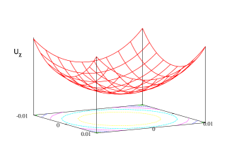
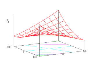
Figure 2: The form of $U_{\chi}$ in the complex $\chi$-plane near the origin. On the left: $m_{1}$ is small and the potential is almast symmetric. On the right: $m_{1}$ is big and this changes the form of the potential, the minimum becomes a saddle point.

For such values of the parameters the non-sphericity of the potential is quite small and there is no preferred direction in the complex $\chi$-plane for the quantum fluctuations generated at inflationary stage when $m_{eff}<H$. On the other hand, when inflation is over and $\chi$ approaches its equilibrium point at $\chi=0$, the non-sphericity of the potential is essential for creation of the noticeable angular momentum, i.e. for generation of baryonic charge asymmetry in the sector of the scalar baryon $\chi$, see Fig. 3.

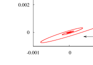
Figure 3: The typical picture of the evolution of $\chi$ in the complex $\chi$-plane, $\chi=\chi_{1}+i\chi_{2}$. The zoomed part inside the figure shows the rotation around the absolute minimum after the end of inflation.

Thus to summarize. As it is already described above, during inflation, when $\Phi$ is close to $\Phi_{1}$, the quantum fluctuations of $\chi$ become large enough to overshoot the barrier and field $\chi$ starts classical rolling down towards the deeper minimum, $\chi^{(2)}(t)$. As one can see in Figs. 3 and 4, $\chi$ reaches this minimum, follows its evolution in time, and oscillates around this minimum with decreasing amplitude. At the end of inflation when the minimum of the potential at $\chi=0$ becomes again the only minimum, the field rolls down to the origin along the slope of the potential. Coming close to the origin the field starts to rotate around it due to the angular momentum generated by non-sphericity of the potential, i.e. due to the complex mass terms (see Fig. 3 and the zoomed part inside). To gain a considerable angular momentum the magnitude of this terms at low $\chi$ should be comparable with the others entering equation of motion (9). This is the reason why we have chosen $m_{0}$ only slightly larger than $|m_{1}|$. The term $\sim\chi^{4}$ is not essential near $\chi=0$. The form and slope of the spiral-like trajectory depend on the effective mass of $\chi$. The rotation of $\chi$ around the origin corresponding to the nonzero baryonic charge would be transformed into the baryonic asymmetry of quarks and ultimately of protons and neutrons by B-conserving decays of $\chi$ into (light or massless) fermions. The sign of the asymmetry depends on the direction of the rotation and can be arbitrary because, as we mentioned above the initial value of the phase $\theta$ is uniformly distributed in the interval $[0,2\pi]$. So in this version of the scenario we would expect an equal number of baryonic and antibaryonic bubbles. In slightly complicated models this symmetry between B and anti-B bubbles may be lifted.

The magnitude of the asymmetry inside the B-bubbles can be much larger than canonical value (1). Moreover, if the life-time of $\chi$ noticeably exceeds the life-time of the inflaton, the asymmetry may be even larger than unity, because the energy density of the decay products of the inflaton into relativistic particles would be strongly red-shifted with respect to non-relativistic longer-lived $\chi$-bosons. The baryon asymmetry depends upon the initial value of phase, $\theta$, of field $\chi$. According to the presented above arguments, $\theta$ should be homogeneously distributed in the interval $[0,2\pi]$. Thus the asymmetry between $\chi$ and anti-$\chi$ inside the bubbles may vary from zero to the maximum value $B_{\chi}\sim m|\chi|^{2}$. The baryon asymmetry $\beta$ depends upon the ratio of the energy density of $\chi$, $\rho_{\chi}\sim m^{2}|\chi|^{2}$, at the moment of $\chi$ decay to the background cosmological energy density. If $\chi$ decayed when the background relativistic matter was strongly red-shifted, the energy density inside the bubble would be dominated by the energy density of $\chi$ and the ratio of the baryonic charge density to the entropy density inside the bubbles would be about

$$\beta_{B}\sim\frac{m|\chi|^{2}}{\left(m^{2}|\chi|^{2}\right)^{3/4}}=\left(\frac{|\chi|}{m}\right)^{1/2}\;.$$ (18)

This value may be much larger than unity.

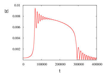
Figure 4: Evolution of $|\chi|$ in time. The field rolls down toward the deeper minimum, oscillates there following the evolution of the minimum, rolls back to the origin and starts to rotate around it.

4 Distributions of bubbles over size and mass

The process of the B-bubble formation predominantly took place when the effective mass of $\chi$-field, eq. (7), was smaller than the Hubble parameter (10). It roughly corresponds to

$$\lambda_{1}(\Phi-\Phi_{1})^{2}<\frac{4\pi m_{\Phi}^{2}\Phi^{2}}{3m_{Pl}^{2}}\;.$$ (19)

During this period we consider $\chi$ as a massless field and estimate how fast its quantum fluctuations rose. Here we follow ref. [16], which in turn was based on the diffusion equation governing evolution of the quantum fluctuations, derived in paper [20].

Qualitatively the picture looks as following. “Massless” field $\chi$ “Brownian” moves from zero with the average displacement given by eq. (2). If $\chi$ exceeds a certain value $\chi_{c}$, after which the motion of $\chi$ away from the origin would be governed by its potential (5), the motion turns into classical roll down to the second minimum $\chi_{2}$ of this potential. The boundary value when the evolution of $\chi$ turns from the quantum regime into the classical one can be found from the condition $U^{\prime\prime}(\chi,\Phi)=H^{2}$, or approximately:

$$2\lambda_{2}|\chi_{c}|^{2}\ln\left(\frac{|\chi_{c}|^{2}}{\sigma^{2}}\right)\approx\frac{4\pi m_{\Phi}^{2}\Phi_{1}^{2}}{3m_{Pl}^{2}}\;.$$ (20)

Those $\chi$’s which were able to reach this value would give birth to B-bubbles. Earlier formed B-bubbles would have considerably larger sizes because their creation took place at inflationary period and the ratio of the radii of two bubbles crated at $t_{1}$ and $t_{2}$ would be:

$$r_{1}/r_{2}=\exp\left(\int_{t_{1}}^{t_{2}}Hdt\right)\;.$$ (21)

Let us introduce the probability distribution ${\cal P}(\chi,t)$ of quantum fluctuations to have the value $\chi=\chi_{1}+i\chi_{2}$ at time $t$. We assume that it is normalized to unity:

$$\int_{-\infty}^{+\infty}d\chi_{1}d\chi_{2}{\cal P}(\chi,t)=1\;.$$ (22)

The probability of B-bubble formation per unit time and per unit volume can be parametrized as:

$$\frac{dW}{dtdV}=\int d\chi_{1}d\chi_{2}\mu^{4}{\cal P}(\chi,t)\;,$$ (23)

where $\mu$ is a parameter with dimension of mass. It is natural to expect that $\mu=H$. There are simply no other parameter in the massless limit. At inflationary stage we may assume that $H\approx const$. The initial size of a B-bubble should be of the order of $r_{in}\sim 1/H$. Hence the fraction of the total volume occupied by the bubbles is

$$\nu(t)=\int^{t}_{t_{in}}dt^{\prime}H\int_{\chi_{c}}^{\infty}d\chi_{1}d\chi_{2}{\cal P}(\chi,t^{\prime})\;,$$ (24)

where we may formally take $t_{in}=-\infty$ but in reality it is determined by the condition $m_{eff}\leq H$. To obtain the above result we took into account that the bubbles formed at time $t^{\prime}$ exponentially expand together with the rest of the universe and their radius rises as $r(t)=H^{-1}a(t)/a(t^{\prime})$, where $a(t)$ is the cosmological scale factor. So after formation their volume fraction remains constant.

Correspondingly, we find that the volume distribution of B-bubbles, or better to say, their number density as a function of their size would have the form:

$$N(r,t)\sim\int_{\chi_{c}}^{\infty}d\chi_{1}d\chi_{2}{\cal P}\left(\chi,t^{\prime}(r,t)\right)\;,$$ (25)

where $t^{\prime}(r,t)$ can be found from the equation: $a(t)/a(t^{\prime})=rH$ and $H$ is the Hubble parameter during inflation. In particular, if we remain at inflationary stage, then $a(t)=\exp(Ht)$ and $t^{\prime}(r,t)=t-H^{-1}\ln(rH)$. This derivation is valid for constant $H$. In realistic situation $H$ drops down with time. We will consider this case below.

As is argued in ref. [16] (see also this section below), for the quadratic potential $U=m^{2}_{eff}(t)|\chi|^{2}$ the probability distribution has the Gaussian form:

$${\cal P}\left(\chi,t\right)=C(t)\exp\left[-|\chi^{2}|/2\langle\chi^{2}\rangle\right]\;,$$ (26)

where $C(t)$ is determined by the normalization condition (22). The mean square width of the distribution is given by

$$\langle\chi^{2}\rangle=\frac{H^{3}}{4\pi^{2}}\int_{t_{i}}^{t}dt^{\prime}\exp\left(-\frac{2}{3H}\int_{t^{\prime}}^{t}dt^{\prime\prime}m^{2}_{eff}(t^{\prime\prime})\right)\;.$$ (27)

When $\Phi$ is close to $\Phi_{1}$, the effective mass behaves as $m_{eff}^{2}(t)\approx m_{0}^{2}+m_{3}^{4}(t-t_{1})^{2}$, where $t_{1}$ is the moment when $\Phi=\Phi_{1}$. This case was analyzed in ref. [16], where it was shown that both the bubble distributions over length and mass have log-normal form. In particular,

$$\frac{dn}{dM}=C_{M}\exp\left[-\gamma\,\ln^{2}(M/M_{0})\right]\;,$$ (28)

where $C_{M}$, $\gamma$, and $M_{0}$ are some constant parameters, which can be expressed through the parameters of the model. For phenomenological applications we take $C_{M}$, $\gamma$, and $M_{0}$ as almost free parameters with the values which are in the interval dictated by the “reasonable” values of the coupling constants and masses of $\chi$ and $\Phi$. Notice that a modification of this distribution by a power factor, $M^{b}$, or, which is the same, by a log term in the exponent, $\exp(b\ln M)$ lead to the same log-normal form of the distribution (28) with the corresponding change of the values of the parameters.

The log-normal form of the bubble distribution was derived in ref. [16] under simlifying assumption of a constant Hubble parameter during inflation. In many realistic situations $H$ depends upon time and drops down practically to zero when inflation ends at $t=t_{e}$:

$$H(t)\equiv H_{1}h(\tau)=H_{1}[1-h_{1}(\tau-\tau_{1})].$$ (29)

Here $\tau=H_{1}t$ and $t_{1}$ is the moment when $\Phi=\Phi_{1}$ and $h_{1}=1/(\tau_{e}-\tau_{1})\ll 1$. For such $H(t)$ the size of the bubble created at $t=t_{p}$ rises as

$$l(\tau,\tau_{p})=l_{in}\exp\left[\int_{\tau_{p}}^{\tau}d\tau h(\tau)\right]\;.$$ (30)

Correspondingly, the size of the bubble at the end of inflation will be

$$l(\tau_{e},\tau_{p})=l_{in}\exp\left[\left(\tau_{e}-\tau_{p}\right)\left(1+h_{1}\tau_{1}-\frac{1}{2}h_{1}\left(\tau_{e}+\tau_{p}\right)\right)\right]\;.$$ (31)

From this equation we see that the bubbe size is related to the production moment as

$$\tau_{p}=h_{1}^{-1}\left(1+h_{1}\tau_{1}-\sqrt{2h_{1}\ln lH_{1}}\right)\;.$$ (32)

The distribution of the bubbles over their size can be written:

$$W(l)=C_{l}\exp\left[-\gamma\left(\tau_{e}-\tau_{1}-\sqrt{2(\ln l)/h_{1}}\right)^{2}\right]\;,$$ (33)

After some modifications this expression can be rewritten as

$$W(l)=C_{l}\exp\left[-\gamma(\tau_{e}-\tau_{1})^{2}\left(1-\sqrt{\frac{2}{h_{1}(\tau_{e}-\tau_{1})^{2}}\ln l}\right)^{2}\right]\;.$$ (34)

Now after simple algebra we find that the distribution over $l$ again has the log-normal form:

$$W(l) = C_{l}\exp\left[-\gamma(\tau_{e}-\tau_{1})^{2}\left(1-\sqrt{1+\frac{\ln l/l_{0}}{\ln l_{0}}}\right)^{2}\right]$$ (35)

$$\simeq C_{l}\exp\left[-\tilde{\gamma}\ln^{2}\left(l/l_{0}\right)\right]\;,$$

where $l_{0}=\exp[h_{1}(\tau_{e}-\tau_{1})^{2}/2]$ and $\tilde{\gamma}=\gamma/h_{1}^{2}(\tau_{e}-\tau_{1})^{2}$.

The equation governing the evolution of the quantum fluctuations of a real scalar field was derived in ref. [20]. Following this derivation we can conclude that the probability distribution for a complex field $\chi$ in potential $U(\chi)$ in (quasi) De Sitter space-time with the Hubble parameter $H$ satisfies practically the same equation

$$\frac{\partial{\cal P}}{\partial t}=\frac{H^{3}}{8\pi^{2}}\sum_{k=1,2}\frac{\partial^{2}{\cal P}}{\partial\chi_{k}^{2}}+\frac{1}{3H}\sum_{k=1,2}\frac{\partial}{\partial\chi_{k}}\left[{\cal P}\frac{\partial U}{\partial\chi_{k}}\right]\;,$$ (36)

where $\chi_{1,2}$ are the real and imaginary parts of field, $\chi=\chi_{1}+i\chi_{2}$, respectively.

We decompose $\chi_{k}$ into classical part $\chi^{(0)}_{k}$ and quantum fluctuations,

$$\chi_{k}=\chi^{(0)}_{k}+\eta_{k}\;.$$ (37)

At the initial stage, when $\Phi$ was far from $\Phi_{1}$, the effective mass of $\chi$ was large and quantum fluctuations were small near $\chi^{(0)}_{k}=0$. In this case the potential governing their evolution can be approximated as the quadratic one:

$$U_{q}=\frac{1}{2}m_{ij}^{2}\eta_{i}\eta_{j}\;,$$ (38)

with the effective mass:

$$m_{ij}^{2}=\left.\frac{\partial^{2}U}{\partial\chi_{i}\partial\chi_{j}}\right|_{\chi_{i}=\chi_{i}^{(0)}}\;.$$ (39)

Due to the last two terms in eq. (5) the potential is not symmetric with respect to the phase rotation of $\chi$ and the matrix $m_{ij}$ may contain off-diagonal terms, $m_{12}\neq 0$. However by a suitable redefinition of $\chi\rightarrow\exp(i\phi)\chi$ we can eliminate imaginary part of $m$ and make $m_{ij}$ diagonal.

For a quadratic potential eq. (36) can be solved in the form:

$${\cal P}={\cal A}(t)\exp(-a_{ij}\eta_{i}\eta_{j})\;,$$ (40)

where $a_{ij}$ is a symmetric $2\times 2$ matrix and ${\cal A}$ is determined by the normalization condition (22):

$${\cal A}(t)=\frac{1}{\pi}\sqrt{\det{a}}\;.$$ (41)

After simple algebra, comparing terms of zeroth and second order in $\chi_{i}\chi_{j}$, we obtain in the matrix form:

$$\frac{1}{2}{\rm tr}[a^{-1}\dot{a}] = -\frac{H^{3}}{4\pi^{2}}{\rm tr}[a]+\frac{1}{3H}{\rm tr}[m^{2}]\;,$$ (42)

$$\dot{a} = -\frac{H^{3}}{2\pi^{2}}\,a^{2}+\frac{2}{3H}\,am^{2}\;.$$ (43)

There are three unknown functions, $a_{ij}(t)$ and four equations (taken into account symmetry of matrix $a$). Still the system is not over-determined. If we multiply the second equation by matrix $a^{-1}$ and take trace, we obtain the first equation.

As we mentioned above, the mass matrix $m^{2}$ can be made diagonal by phase rotation of $\chi$. Correspondingly matrix $a$ becomes diagonal too and the equations for $a_{11}$ and $a_{22}$ components decouple. Introducing $\kappa_{j}=1/a^{-1}_{jj}$ (no summation), we obtain the linear equations:

$$\dot{\kappa}_{j}+\frac{2}{3H}\,m_{j}^{2}\kappa_{j}=\frac{H^{3}}{2\pi^{2}}\;.$$ (44)

These equations can be integrated by quadratures for arbitrary $m^{2}(t)$ and $H(t)$ but it may be simpler to integrate them numerically directly (see Fig. 5).

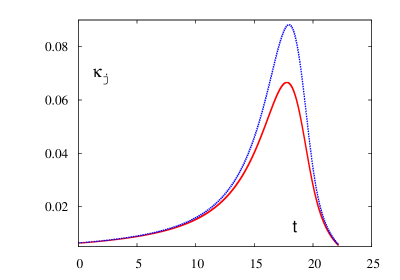
Figure 5: The variation of the mean square values $\kappa_{j}$ as a function of time. All quantities are normalized to $H_{1}$, i.e. $t\rightarrow H_{1}t$ and $\kappa_{j}\rightarrow\kappa_{j}/H_{1}^{2}$. This result is obtained with effective mass (39) using potential (5).

This result allows to calculate the probability distribution for sufficiently small quantum part of $\chi$, when quadratic approximation is valid. As we have already mentioned, when $\chi$ reached the critical value $\chi_{c}$ (20) its evolution would be governed by classical equation (9) with the potential which is dominated by log-quartic term $\lambda_{2}|\chi|^{4}\ln|\chi|^{2}/\sigma^{2}$. These terms in the potential become essential rather early, still at the quantum regime. To get a qualitative understanding of the impact of this terms we proceed as follows. We approximate the potential by

$$U\approx m_{eff}^{2}|\chi|^{2}-\lambda_{2}|\chi|^{4}\;,$$ (45)

where $m_{eff}^{2}=m_{0}^{2}+\lambda_{1}(\Phi-\Phi_{1})^{2}$. We neglect the last two aspherical terms in the potential (5) because their role at this stage is not important. For a spherically symmetric potential $U=U(|\chi|)$ the probability distribution depends only upon $|\chi|$ and we will look for the approximate solution in the form:

$${\cal P}(\chi,t)={\cal A}(t)\left[1+b(t)|\chi|^{4}\right]\,\exp\left[-|\chi|^{2}/\kappa(t)\right]\;,$$ (46)

assuming that terms containing $b(t)$ with higher powers of $\chi$ are small.

The normalization condition now leads to:

$${\cal A}=\frac{1}{\pi\kappa(1+2b\kappa^{2})}\;.$$ (47)

Substituting this expression into eq. (36) and neglecting terms of higher order in $b$ and sixth power of $\chi$ we find for zero, second, and fourth powers of $\chi$ respectively (only two out of these three equations are independent):

$$\frac{\dot{\kappa}}{\kappa} = \frac{H^{3}}{2\pi^{2}\kappa}\left(1+4b\kappa^{2}\right)-\frac{4}{3H}\,\left(m_{eff}^{2}+4\lambda_{2}\kappa\right)\;,$$ (48)

$$\dot{b} = -\frac{2H^{3}b}{\pi^{2}\kappa}+\frac{8\lambda_{2}}{3H\kappa}+\frac{8m^{2}_{eff}b}{3H}\;.$$ (49)

It is easy to solve these equations numerically. As expected, $\kappa$ becomes a few percent larger at $\Phi\sim\Phi_{1}$, i.e. the additional negative quartic term stimulates the growth of fluctuations.

5 Density perturbations created by B-bubbles and their evolution

As it was mentioned in ref. [16], B-bubbles could create large isocurvature density perturbations at relatively small scales. The spectrum of angular fluctuations of cosmic microwave background radiation (CMBR) excludes noticeable isocurvature perturbations with wave lengths larger than approximately 10 Mpc [26, 27], but at smaller scales they are allowed and may even be very large.

In the considered model there are two mechanisms of the density perturbations, which were operative at different cosmological epochs. Inside B-bubbles the baryon asymmetry, $\beta$, may be much larger than the observed value $\beta\approx 6\cdot 10^{-10}$. Such inhomogeneous distribution of the baryon number would not lead to noticeable density perturbations till quarks remained ultra-relativistic, i.e. till the QCD phase transition. In this way relatively large objects with high density contrast could be created. This was considered in ref. [16], where stellar and larger mass objects were studied. There is another possibility to perturb the cosmological energy density disregarded in ref. [16]. This mechanism operated at an earlier cosmological period and might lead to perturbations with much smaller wave lengths and masses, $M\ll M_{\odot}$, than those created at the QCD phase transition. Here we consider in detail both possibilities.

Let us first discuss the early stage when the B-bubbles were created. Initially, at inflationary stage, the density contrast between low and high $\chi$-regions was negligible, first, because the energy density of $\chi$ is assumed to be strongly subdominant with respect to the inflaton one. Second, the bubble formation did not lead to a density contrast at the moment of formation simply because of energy conservation. The energy density contrast $\delta\rho$ between the bubbles and the rest of the universe remained small till the end of inflation. After inflation is over and the inflaton decayed into (predominantly) relativistic particles, the situation might change, if the life-time of $\chi$ is larger than the time of the inflaton decay. Outside the bubbles there would be only relativistic matter, while inside the bubbles there would be a mixture of nonrelativistic and relativistic matter. Indeed, in the course of the subsequent cosmological evolution the equation of state of $\chi$ would be different for small $\chi$ near zero and for large $\chi$ staying in the second minimum of $U(\chi,\Phi)$. At this stage the energy density of $\chi$ would behave as vacuum-like energy. When this minimum disappeared, $\chi$ started to oscillate around zero in essentially quadratic potential. So its equation of state became that of nonrelativistic matter and its energy density was red-shifted as the scale factor cube.

To illustrate the evolution of the density perturbations in the considered model let us assume that there are two large (larger than horizon) pieces of the universe, the bulk with the relativistic equation of state, $p_{r}=\rho_{r}/3$, and a bubble with a large value of $\chi$ with a mixture of relativistic and a small fraction of non-relativistic matter, $\rho_{nr}^{in}=\epsilon\rho_{r}^{in}$. The energy density inside the bubble evolves as:

$$\rho_{inside}=\frac{\rho_{r}^{in}}{x^{4}}+\frac{\rho_{nr}^{in}}{x^{3}}=\frac{\rho_{r}^{in}}{x^{4}}\left(1+\epsilon x\right)\;,$$ (50)

where $x=a/a_{in}$ is the ratio of the running cosmological scale factor to its initial value.

We can find the dependence of the scale factor on time solving the Friedmann equation:

$$\left(\frac{\dot{x}}{x}\right)^{2}=\frac{8\pi}{3m_{Pl}^{2}}\,\left(\frac{\rho_{r}^{in}}{x^{4}}+\frac{\rho_{nr}^{in}}{x^{3}}\right)\;.$$ (51)

Technically simpler is to solve this equation in terms of conformal time, $d\tau=dt/a(t)$:

$${a}=a_{eq}\left(2\eta+\eta^{2}\right)\;,$$ (52)

where $a_{eq}=a_{in}/\epsilon$ is the value of the scale factor when the energy densities of relativistic and nonrelativistic matter inside the bubble become equal and $\eta=\tau a_{in}/(4t_{in}\epsilon)$. At matter radiation equilibrium $\eta\sim 1$.

In what follows we will use the results presented in book [28] where a very similar case of evolution of density perturbations in the mixed relativistic and nonrelativistic matter is considered. The gravitational potential $\Phi$ satisfies eq. (7.49) of this book with the right hand side which is non-zero because of the difference of equations of state inside and outside the bubble. The solution for $\Phi$ with the initial condition $\Phi(\eta=0)=0$ has the form:

$$\Phi=\frac{\eta}{5}\frac{\eta^{2}+6\eta+10}{(\eta+2)^{3}}\,\frac{\delta S}{S}\;,$$ (53)

where

$$\frac{\delta S}{S}=\frac{3}{4}\,\frac{\delta\rho_{r}}{\rho_{r}}-\frac{\delta\rho_{nr}}{\rho_{nr}}\;.$$ (54)

Notice that the entropy perturbations are not small becasue $\delta\rho_{nr}/\rho_{nr}=1$.

The density perturbations are related to the potential through the equation (7.47) of book [28]:

$$\Delta\Phi-3{\cal H}\left(\Phi^{\prime}+{\cal{H}}\Phi\right)=4\pi G_{N}a^{2}\delta\rho,$$ (55)

where the Laplacian term in the l.h.s. can be neglected for large wave length of perturbations. Thus $\delta\rho/\rho\simeq 2\Phi$.

From this equation we find that asymptotically at MD stage, i.e. for $\eta\gg 1$, the density perturbations tend to a constant value

$$\left.\frac{\delta\rho}{\rho}\right|_{MD}=-\frac{2}{5}\,\frac{\delta S}{S}\approx\frac{2}{5}\;.$$ (56)

For small $\eta$, i.e. at RD stage the perturbations rise linerly with conformal time:

$$\left.\frac{\delta\rho}{\rho}\right|_{RD}=-\frac{\eta}{2}\frac{\delta S}{S}\approx\frac{\eta}{2}\;.$$ (57)

At some moment field $\chi$ should decay into relativistic matter and after that both inside and outside the bubble equations of state would be identical, those of relativistic matter, $p=\rho/3$. After decay the developed density perturbations would stay constant, see eq. (7.59) of ref. [28]. In the instant decay approximation the initial value of the constant potential and density contrast can be read off equations (56) and (57). To be more accurate we can proceed as follows. We have to solve the system of the following two equations, assuming that all nonrelativistic matter is created by $\chi$-field:

$$\dot{\rho}_{\chi}+3H\rho_{\chi}+\Gamma_{\chi}\rho_{\chi}=0\;,$$ (58)

$$\dot{\rho}_{r}+4H\rho_{r}-\Gamma_{\chi}\rho_{\chi}=0\;,$$ (59)

where $\Gamma_{\chi}=1/\tau_{\chi}$ is decay rate of field $\chi$ into light particles.

The solution of equation (58):

$$\rho_{\chi}=\frac{\rho_{\chi}^{in}}{x^{3}}\exp{(-\Gamma_{\chi}t)}\;.$$ (60)

Equation (59) would be simplified in terms of the new function $\rho_{r}=\rho_{r}^{in}\zeta/x^{4}$ with the initial value $\zeta=1$ at $t=0$, or $x=1$. The resulting equation takes the form:

$$\dot{\zeta}=\epsilon\Gamma_{\chi}\,xe^{-\Gamma_{\chi}t}\;,$$ (61)

where $x=x(t)$ is determined by eq. (51) but instead of $\rho$ given by eq. (50) we have to substitute there the solutions of eqs. (58,59). A solution to this system of equations can be done numerically.

We see that the density contrast for superhorizon perturbations initially grows up but asymptotically tends to a constant value. When the bubble size becomes smaller than cosmological horizon, the further evolution of the bubble depends on the magnitude of the density contrast at the moment of the horizon crossing, $\Delta_{h}$. If $\Delta_{h}\sim 1$, such bubbles would form primordial black holes (PBH). For a review of PBH creation see e.g. refs. [29, 30].

We should remember however, that the presented above estimates are true only for small perturbations when first order expansion in perturbed quantities is accurate. As we saw, the estimated perturbations are of the order of unity and so we can trust the calculations only by an order of magnitude.

The mass inside the horizon is

$$M_{h}\sim m_{Pl}^{2}t\;.$$ (62)

So the discussed mechanism allows for formation of PBH with the masses of the order of $M_{BH}\sim 4\cdot 10^{38}(\tau_{\chi}/{\rm sec}){\rm g}$, if the size of the bubble was inflated up to horizon at that moment. An oversimplified estimate of the life-time of $\chi$-boson as $\tau_{\chi}\sim(g^{2}m_{\chi}/4\pi)^{-1}$, where $g$ is the Yukawa coupling constant of $\chi$ to fermions, gives for $g^{2}=0.01$ and $m_{\chi}=10^{8}$ GeV: $M_{BH}\sim 10^{9}$ g. Such light PBHs should evaporate in about one second and would not be important in the present day universe. On the other hand, the life-time estimated above is certainly too short. In supersymmetric theory with conserved $\cal R$-parity the lightest supersymmetric particle (LSP) must be stable. So $\chi$ should either be stable or decay into a massive LSP. For simplicity we will not dwell on the problems related to color conservation and formation of $\chi$ condensate. This discussion can be found e.g. in the reviews [31, 32]. We will assume that $\cal R$-parity is broken and $\chi$ predominantly decays into ordinary particles but with baryonic charge conservation. If this is realized, the life-time may be much smaller than the estimate presented above and PBHs with much larger masses could be created. Since $\cal R$-parity violating effects are only bounded from above, the life-time is allowed to be arbitrary large. Another effect which might result in larger PBH masses is a delayed evaporation of the $\chi$-condensate found in refs. [33, 34]. On the other hand, it is not obligatory to live in a SUSY world but instead we can postulate ad hoc an existence of a new $\chi$-field with the necessary properties and in this case we would be free from the SUSY restrictions. So, one way or another, the considered mechanism can lead to formation of PBH which live long enough to be present in the contemporary universe.

If the density contrast is not sufficient for creation of PBH, the bubble would end up as a more dense piece of relativsitic matter inside the relativistic cosmological backgound. The density contrast $\delta$ inside horizon is known to remains constant or to be more precise, may rise logarithmically (see e.g.  [35, 28, 36]), while outside horizon it drops down as $1/t$, as is mentioned above. The bubbles might be dissolved by diffusion but in relativstic regime the mean free path is about $l_{free}\sim 1/(\alpha^{2}T)$ and thus remains small in comparizon with the bubble size which rises with the cosmological scale factor $a\sim 1/T$. So if the bubble size was initially larger than $l_{free}$ it remains such during all relativistic stage.

The second period when the perturbation in baryonic number density could be transformed into the energy density perturbation, happened after the QCD phase transition (p.t.) from deconfinement to confinement phase. After this p.t. practically massless quarks turned into heavy baryons and the baryonic number fluctuations would be transformed into the energy density perturbations. If the baryon asymmerty inside the bubble has the value $\beta_{B}$ the density contrast after the QCD p.t. would be

$$\Delta=\frac{\delta\rho}{\rho}=\frac{\beta n_{\gamma}m_{p}}{(\pi^{2}/30)g_{*}T^{4}}\approx 0.07\beta_{B}\,\frac{m_{p}}{T}\;,$$ (63)

where temperature $T$ should be smaller than the temperature of the QCD p.t., $T_{QCD}$. The latter is rather poorly known and according to different estimates it varies between 100-200 MeV. The quoted results, however, were obtained for zero or negligible baryonic chemical potential, $\mu_{B}$. In our case $\mu_{B}$ could be large, but not large enough to shift the value of $T_{QCD}$ for more then $2\%$ [37, 38].

The bubble with $\Delta$ (63) larger than unity at horizon crossing would form PBH but now (in contrast to the case consided above) with very large masses, starting from a few solar masses to possibly millions of $M_{\odot}$, if the bubble size is so large that it enters horizon at, say, $t=10-100$ s, see eq. (62) with $t\geq 10^{-5}$ s.

If at horizon crossing $\Delta_{B}<1$, the bubble evoluton is detemermined by the relation between its size, $l_{B}$ and the Jeans wave length:

$$\lambda_{J}=c_{s}\left({\frac{\pi m_{Pl}^{2}}{\rho}}\right)^{1/2}\;,$$ (64)

where $\rho$ is the background energy density and $c_{s}$ is the speed of sound. For relativistic plasma $c_{s}=1/\sqrt{3}$ and the Jeans wave length is close to horizon $l_{h}=2t$.

The Jeans mass is defined as

$$M_{J}=\frac{4\pi}{3}\rho{\lambda_{J}}^{3}\;.$$ (65)

As is well known, the regions with $M>M_{J}$ or with $\lambda>\lambda_{J}$ would decouple from the cosmological expansion and form gravitationally binded systems. In the regions with smaller mass gravitational instability is not developed and the perturbations oscillate.

In the usual cosmological plasma the Jeans mass and wave length are very large before hydrogen recombination because of very small baryon asymmetry or a very large entropy per baryon, see e.g. book [39]. After $e^{+}e^{-}$ annihilation, i.e. at $T<0.1$ MeV the baryonic Jeans mass was about $10^{4}M_{\odot}$ and rose up to $10^{18}M_{\odot}$ till hydrogen recombination. After recombination it sharply drops down to $10^{6}M_{\odot}$ and continue to decrease as $a(t)^{-3/2}$.

In our case the entropy per baryon is not huge and the picture is quite different. The energy density inside B-bubble, assuming that baryons are nonrelativstic, is

$$\rho_{B}=n_{B}m_{p}+(\pi^{2}/30)g_{*}T^{4}\;,$$ (66)

where $n_{B}$ is the baryon nuber density and $g_{*}$ is the efective number of the relativistic species. For photons $g_{*}=2$ and for equilibrium photons and $e^{\pm}$ pairs $g_{*}=5.5$.

The pressure density is equal to:

$$P_{B}=(\pi^{2}/90)g_{*}T^{4}+n_{B}T\;.$$ (67)

For adiabatic perturbations the ratio of the baryon number density to the photon number density remains constant if entropy release by $e^{+}e^{-}$-annihilation is neglected. Disregarding this and similar efects we obtain by an order of magnitude:

$$c_{s}^{2}=\frac{1}{3}\,\frac{T}{T+m_{p}\beta}\;.$$ (68)

Correspondingly the Jeans mass at the QCD phase transition would be about $10M_{\odot}$ if $\beta=1$. Assuming that the B-bubble is dominated by nonrelativsitc matter we find that with further cosmological expansion $M_{J}$ would drop as $a^{3/2}$ because the energy density of baryons decreases as $a^{-3}$ and the temperature of mixture of nonrelativistic baryons and photons decreases as $T\sim 1/a^{2}$. For smaller $\beta$ the Jeans mass can be significantly larger.

Thus we see that after the QCD p.t. PBH with masses starting from a few solar masses and much higher can be created as well as gravitationally bound objects with masses from a fraction of the solar mass up to thousands or more solar masses could emerge. These early formed objects would be made either from matter or antimatter with equal probability.

6 Observational bounds and implications

There are two features of the considered here model which may make it cosmologically and astrophysically interesting.

First, according to the presented scenario all cosmological dark matter can be made out of baryons and antibaryons in the form of compact stellar type objects or primordial black holes. These PBHs can be rather light, e.g $10^{15}-10^{20}$ g or very heavy, up to millions solar masses. The number density of light PBHs is restricted by the condition that their evaporation should not create too strong electromagnetic radiation to exceed the observed one. The analysis, summarized in ref. [29, 41] excludes PBHs in a large interval of masses as the dominant part of cosmological DM. However, the conclusion of ref. [41] is valid only for a narrow spectrum of PBH masses, when all PBHs have practically equal masses. In our case the mass spectrum can be sufficiently wide to allow for light PBHs to be the dominant dark matter (DM) particles and to avoid condradiction with the observed cosmic electromagnetic radiation.

A possible manifestation of PBH with masses around $10^{16}-10^{17}$ g may be 0.511 MeV line observed in the Galactic bulge  [42, 43, 44, 45, 46, 47, 48] and probably from the halo [49]. As argued in ref. [50] such PBHs may explain the observed flux and be abundant enough to make all cosmological DM. As was observed recently the source of this line is asymmetric with respect to the galactic center and is correlated with the observed X-ray binaries [51]. It make probable that the origin of the annihilated positrons are these low mass X-ray binaries, though the estimated intensity of the line is about a half of the observed. On the other hand, the distribution of PBHs may be also asymmetric and correlated with the distribution of the binaries.

If the central mass in the distribution (28) is close to the solar mass, we would expect quite heavy cosmological dark matter “particles” made out of heavy PBH and dead or low luminocity stars with masses of a fraction of solar mass and may be much larger. An analysis of the evolution of such stellar like objects formed in the early universe will be made elsewhere. As is argued in ref. [16], an interesting feature of this scenario is that on the high mass tail of the distribution (28) there may be superheavy PBH with masses of millions solar masses. We can choose the parameters of the distibuiton such that the number of the superheavy BH would be equal to the number of the observed large galaxies. So the model explains an early quasar creation which may seed galaxy formation, as it was recently argued [52]. To make a better qualitative statement one should study the amount of matter accretion during life time of these superheavy BHs from the moment of their creation when the universe was about 1 sec old till practically present time.

The observed in microlensing searches stellar mass low luminocity objects (MACHOS) could be such solar mass PBH or dead very early stars and antistars. According to ref [53], such objects may make at most 40% of the total galactic DM. However, again this bound is true only for narrow mass spectrum of MACHOS. If the latter is sufficiently wide PBH can be safely put below the upper bound curve and make 100% of galactic DM. (A little here, a little there makes unity.)

An argument against very heavy DM particles is presented in ref. [54], according to which the objects with masses above $10^{-2}M_{\odot}$ may constitute not more than 88% of cosmological DM at 95% confidence level. So we should either allow for 12% to be in the form of relatively light PBHs or planet-like objects with masses below $2\cdot 10^{31}$ g or hope that 95% CL is not strong enough to exclude very heavy PBHs.

The second possibly testable feature of the model is a prediciton of noticeable amount af antimatter, in the form of compact stellar-like objects. Out of $\Omega_{DM}=0.25$ a half may consist of antimatter. So we have almost charge symmetric universe with the amount of matter $\Omega_{B}\approx 0.16$ and that of antimatter $\Omega_{\bar{B}}\approx 0.12$. Of course the bulk of baryonic and antibaryonic matter can be inside PBHs and thus unboservable (except for its gravity), however, it is not excluded that a noticeable amlount of antimatter is in the form of evolved anti-stars or antimatter clouds. There are quite strong bounds on the amount of cosmic antimatter in the usual form. For example, the nearest antigalaxy mast be at least at the distance of 10 Mpc [55]. In baryosymmeteric cosmology the nearest domain of antimatter should be at the distance of (a few) Gygaparsecs [14]. Bounds on the amount of galactic antimatter in “normal” form in baryo-asymmetric cosmology are discussed in ref. [56, 57, 58]. However, in our case these bounds are not applicable, see ref. [2], and one may expect that roughly a half of the galactic mass is made of antimatter in the form of compact low luminocity stars or PBH situated in the disk and in the halo. Possible antistars in the galactic Bulge may be sources of the observed positrons [2].

In the regions with high (anti)baryonic number density primordial nucleosynthesis (BBN) would lead to quite diferent amount of light elements. There would be practically no deuterium, somewhat larger amount of ${}^{4}He$ and ${}^{7}Li$, and anomallously larger abundances of heavier elements which practically are not produced in the standard BBN [59, 60, 61]. This feature can indicate that a cloud or a stellar type objects with anomalous light element abundances may consist of antimatter.

According to ref. [62, 63] the moment of recombination is sensitive to the spatial distribution of baryonic matter and it might be helpful for restriction of the model parameters or its confirmation.

For very simple form of the interaction between $\chi$ and the inflaton field (3) the log-normal mass spectrum of BBs has maximum at some $M_{0}$ which can be either close to normal stellar mass or much smaller, say, $10^{15}-10^{20}$ g. However, with a minor modification of the discussed model we can obtain a multi-maxima spectrum with several values of $M_{0}$. To achieve that we need to modify the interaction of $\chi$ with the inflaton as

$$U_{int}=\lambda_{k}\Pi_{j}^{k}(\Phi-\Phi_{j})^{2}/m_{Pl}^{(2k-1)}.$$ (69)

Such an interaction may emerge from non-renormalizble Planck scale physics.

7 Conclusions

We reconsidered and further developed the scenario of ref. [16] and argued that a simple coupling of the Affleck-Dine scalar baryon to the inflaton may lead to an efficient creation of PBHs either with relatively small masses, $M_{BH}=10^{14}-10^{20}g$, or much larger, $M_{BH}\geq M_{\odot}$. The predicted log-normal mass spectrum of PBH (28) very much differ from the power law one which could be created by other mechanisms considered in the existing literature. This difference is crucial for relaxing the observational bounds on PBH abundance. The suggested mechanism may explain formation of all observed heavy black holes from millions to thousands or tens solar masses. There is no unique and compelling explanation in the existing literature. There is an interesting possibility that all cosmological DM is made of PBH or compact stellar mass objects (early formed and now dead stars) with log-normal mass spectrum. In particular, the observed MACHOS may be solar mass PBHs, or dead (anti)stars.

In the simplest version the mechanism considered here leads to significant creation of astronomical objects made of antimatter. Such objects should have anomalay abundances of (primordially formed) light elements. The search for cosmic antimatter [64], if successed would be crucial for the conformation of the scenarion.

8 Acknowlidgment

We thank V. Mukhanov for the discussion on the evolution of the cosmological density perturbations and A. Drago for a kind conversation about the QCD phase transition. MK thanks N. Suyama for helpful discussion. The work is supported by Grant-in-Aid for Scientific Research from the Ministry of Education, Science, Sports, and Culture (MEXT), Japan, No. 14102004 (M.K.). This work was supported by World Premier International Research Center Initiative WPI Initiative), MEXT, Japan.

References

- [1] D. Casadei, (2004), astro-ph/0405417, revised version of 2008.
- [2] C. Bambi and A. D. Dolgov, Nucl. Phys. B784, 132 (2007), astro-ph/0702350.
- [3] A. D. Sakharov, Pisma Zh. Eksp. Teor. Fiz. 5, 32 (1967).
- [4] A. D. Dolgov, Published in *Varenna 2005, CP violation*, Varenna, Italy, 19-29 Jul , 407 (2005), hep-ph/0511213.
- [5] T. D. Lee, Phys. Rept. 9, 143 (1974).
- [6] Y. B. Zeldovich, I. Y. Kobzarev, and L. B. Okun, Zh. Eksp. Teor. Fiz. 67, 3 (1974).
- [7] R. W. Brown and F. W. Stecker, Phys. Rev. Lett. 43, 315 (1979).
- [8] K. Sato, Mon. Not. Roy. Astron. Soc. 195, 467 (1981).
- [9] K. Sato, Phys. Lett. B99, 66 (1981).
- [10] R. N. Mohapatra and G. Senjanovic, Phys. Rev. D20, 3390 (1979).
- [11] R. N. Mohapatra and G. Senjanovic, Phys. Rev. Lett. 42, 1651 (1979).
- [12] V. A. Kuzmin, M. E. Shaposhnikov, and I. I. Tkachev, Phys. Lett. B105, 167 (1981).
- [13] V. A. Kuzmin, I. I. Tkachev, and M. E. Shaposhnikov, Pisma Zh. Eksp. Teor. Fiz. 33, 557 (1981).
- [14] A. G. Cohen, A. De Rujula, and S. L. Glashow, Astrophys. J. 495, 539 (1998), astro-ph/9707087.
- [15] V. M. Chechetkin, M. Y. Khlopov, and M. G. Sapozhnikov, Riv. Nuovo Cim. 5N10, 1 (1982).
- [16] A. Dolgov and J. Silk, Phys. Rev. D47, 4244 (1993).
- [17] I. Affleck and M. Dine, Nucl. Phys. B249, 361 (1985).
- [18] A. D. Linde, Phys. Lett. B116, 335 (1982).
- [19] A. Vilenkin and L. H. Ford, Phys. Rev. D26, 1231 (1982).
- [20] A. A. Starobinsky, Phys. Lett. B117, 175 (1982).
- [21] A. Dolgov and D. N. Pelliccia, Nucl. Phys. B734, 208 (2006), hep-th/0502197.
- [22] S. R. Coleman and E. Weinberg, Phys. Rev. D7, 1888 (1973).
- [23] S. Fubini, Nuovo Cim. A34, 521 (1976).
- [24] A. S. Goncharov and A. D. Linde, Fiz. Elem. Chast. Atom. Yadra 17, 837 (1986).
- [25] A. D. Linde, The physics of elementary particles and inflationary cosmology (Moscow, Izdatel’stvo Nauka, 1990).
- [26] WMAP, G. Hinshaw et al., (2008), 0803.0732.
- [27] WMAP, E. Komatsu et al., (2008), 0803.0547.
- [28] V. Mukhanov, Cambridge, UK: Univ. Pr. (2005) 421 p.
- [29] B. J. Carr, Lect. Notes Phys. 631, 301 (2003), astro-ph/0310838.
- [30] V. I. Dokuchaev, Y. N. Eroshenko, and S. G. Rubin, (2007), arXiv:0709.0070 [astro-ph].
- [31] R. Barbier et al., Phys. Rept. 420, 1 (2005), hep-ph/0406039.
- [32] D. Kazakov, Surveys High Energ. Phys. 10, 153 (1997).
- [33] A. D. Dolgov and D. P. Kirilova, Sov. J. Nucl. Phys. 50, 1006 (1989).
- [34] A. D. Dolgov and F. R. Urban, Astropart. Phys. 24, 289 (2005), hep-ph/0505255.
- [35] E. W. Kolb and M. S. Turner, Front. Phys. 69, 1 (1990).
- [36] N. Straumann, Annalen Phys. 15, 701 (2006), hep-ph/0505249.
- [37] H. Muller, Nucl. Phys. A618, 349 (1997), nucl-th/9701035.
- [38] M. P. Lombardo, Talk given at the Sixth international conference on perspectives in hadronic physics , Trieste, Italy (2008).
- [39] S. Weinberg, Wiley&Sons, New York, (1972).
- [40] D. H. Oaknin and A. Zhitnitsky, Phys. Rev. D71, 023519 (2005), hep-ph/0309086.
- [41] B. J. Carr, (2005), astro-ph/0511743.
- [42] Johnson, III, W. N. and Harnden, Jr., F. R. and Haymes, R. C., Astrophys. J. 172, L1 (1972).
- [43] Leventhal, M. and MacCallum, C. J. and Stang, P. D., Astophys.J. 225, L11 (1978).
- [44] Purcell, W. R. and Cheng, L.-X. and Dixon, D. D. and Kinzer, R. L. and Kurfess, J. D. and Leventhal, M. and Saunders, M. A. and Skibo, J. G. and Smith, D. M. and Tueller, J., Astrophys.J. 491, 725 (1997).
- [45] P. A. Milne, J. D. Kurfess, R. L. Kinzer, and M. D. Leising, New Astron. Rev. 46, 553 (2002), astro-ph/0110442.
- [46] J. Knodlseder et al., Astron. Astrophys. 441, 513 (2005), astro-ph/0506026.
- [47] P. Jean et al., Astron. Astrophys. 445, 579 (2006), astro-ph/0509298.
- [48] G. Weidenspointner et al., (2006), astro-ph/0601673.
- [49] G. Weidenspointner et al., (2007), astro-ph/0702621.
- [50] C. Bambi, A. D. Dolgov, and A. A. Petrov, (2008), arXiv:0801.2786 [astro-ph].
- [51] G. Weidenspointner et al., Nature 451, 159 (2008).
- [52] T. Di Matteo, J. Colberg, V. Springel, L. Hernquist, and D. Sijacki, (2007), arXiv:0705.2269 [astro-ph].
- [53] EROS-2, P. Tisserand et al., Astron. Astrophys. 469, 387 (2007), astro-ph/0607207.
- [54] R. B. Metcalf and J. Silk, Phys. Rev. Lett. 98, 071302 (2007), astro-ph/0612253.
- [55] G. Steigman, Ann. Rev. Astron. Astrophys. 14, 339 (1976).
- [56] K. M. Belotsky, Y. A. Golubkov, M. Y. Khlopov, R. V. Konoplich, and A. S. Sakharov, (1998), astro-ph/9807027.
- [57] Y. A. Golubkov and M. Y. Khlopov, Phys. Atom. Nucl. 64, 1821 (2001), astro-ph/0005419.
- [58] D. Fargion and M. Khlopov, Astropart. Phys. 19, 441 (2003), hep-ph/0109133.
- [59] S. Matsuura, A. D. Dolgov, S. Nagataki, and K. Sato, Prog. Theor. Phys. 112, 971 (2004), astro-ph/0405459.
- [60] S. Matsuura, S.-I. Fujimoto, S. Nishimura, M.-A. Hashimoto, and K. Sato, Phys. Rev. D72, 123505 (2005), astro-ph/0507439.
- [61] S. Matsuura, S.-i. Fujimoto, M.-a. Hashimoto, and K. Sato, (2007), arXiv:0704.0635 [astro-ph].
- [62] P. Naselsky and D. Novikov, Mon. Not. Roy. Astron. Soc. 334, 137 (2002).
- [63] J. Kim and P. Naselsky, (2008), 0802.4005.
- [64] P. Picozza, Tenth International Conference on Topics in Astroparticle and Underground Physics. Sendai, Japan, September, 2007 and references therein.