Semiclassical analysis of edge state energies in the integer quantum Hall effect

Abstract

Analysis of edge-state energies in the integer quantum Hall effect is carried out within the semiclassical approximation. When the system is wide so that each edge can be considered separately, this problem is equivalent to that of a one dimensional harmonic oscillator centered at $x=x_{c}$ and an infinite wall at $x=0$, and appears in numerous physical contexts. The eigenvalues $E_{n}(x_{c})$ for a given quantum number $n$ are solutions of the equation $S(E,x_{c})=\pi[n+\gamma(E,x_{c})]$ where $S$ is the WKB action and $0<\gamma<1$ encodes all the information on the connection procedure at the turning points. A careful implication of the WKB connection formulae results in an excellent approximation to the exact energy eigenvalues. The dependence of $\gamma[E_{n}(x_{c}),x_{c}]\equiv\gamma_{n}(x_{c})$ on $x_{c}$ is analyzed between its two extreme values $\frac{1}{2}$ as $x_{c}\to-\infty$ far inside the sample and $\frac{3}{4}$ as $x_{c}\to\infty$ far outside the sample. The edge-state energies $E_{n}(x_{c})$ obey an almost exact scaling law of the form $E_{n}(x_{c})=4[n+\gamma_{n}(x_{c})]f(\frac{x_{c}}{\sqrt{4n+3}})$ and the scaling function $f(y)$ is explicitly elucidated.

I Introduction and statement of the problem

The concept of edge states is central for elucidating the physics of quantum Hall and spin quantum Hall systems BH ; MD ; MB ; CK . It is illustrated by considering an electron (mass $m$ and charge $-e$) restricted in two dimensions to a stripe $-\infty<y<\infty,\ \ \ -L_{x}\leq x\leq 0$, and acted upon by a perpendicular magnetic field ${\bf B}=B{\hat{\bf z}}={\bm{\nabla}}{\bf\times}{\bf A}$. At strong enough magnetic field it is reasonable to assume $L_{x}\gg l$, (where $l\equiv\sqrt{\frac{\hbar c}{eB}}$ is the magnetic length), and consider a system with a single edge at $x=0$, where the electron is confined on the half plane $-\infty<y<\infty,\ \ \ -\infty<x\leq 0$. Within the Landau gauge ${\bf A}=(0,-Bx)$, the Schrödinger equation and the corresponding boundary conditions read

$$\frac{1}{2m}[p_{x}^{2}+(p_{y}+\frac{e}{c}Bx)^{2}]\Psi(x,y)=E\Psi(x,y),$$ (1a)

$$\Psi(0,y)=\Psi(-\infty,y)=0.$$ (1b)

Translation invariance along $y$ enables the replacement $p_{y}\to k$ and turns equation (1a) into that of a one dimensional oscillator centered at $X_{c}\equiv kl^{2}$ with hard wall boundary condition at $x=0$. Using $l$ as unit of length, and $\hbar\omega_{c}/2\equiv\hbar^{2}/2ml^{2}$ as unit of energy, the corresponding eigenvalue problem then reads ($-\infty<x\leq 0$) :

$$[-\frac{d^{2}}{dx^{2}}+(x_{c}-x)^{2}]\psi(x)=E\psi(x),$$ (2a)

$$\psi(0)=\psi(-\infty)=0,$$ (2b)

where all quantities are dimensionless and $-\infty<x_{c}={X_{c}}/{l}=kl<\infty$ is the (dimensionless) center of the oscillator, which is considered as a continuous parameter. In the absence of edge, the eigenvalues are simply the Landau energies $E_{n}=2n+1$, independent of $x_{c}$. The presence of edge changes this infinite degeneracy and turns the energies to be dependent on $x_{c}$. When $|x_{c}|$ is small, the oscillator center is close to the edge within a magnetic length so that the corresponding eigenfunctions are localized near the edge of the system at $x=0$ and hence they are referred to as edge states.

The challenge of calculating the eigenstates $\psi_{n}(x;x_{c})$ and the eigenvalues $E_{n}(x_{c})$ is referred to as (partially) restricted harmonic oscillator problem, and dates back several decades ago Aquino . Since confined quantum mechanical systems are ubiquitous, it arises in numerous contexts in physics and chemistry, much beyond the specific edge-state scenario of the quantum Hall effect mentioned above. Formally, the eigenvalue problem (2a,2b) possesses an exact solution in terms of Kummer functions AS , but this solution is hardly useful, as these functions are rather complicated.

The present work focuses on the eigenvalues $E_{n}(x_{c})$ of the Schrödinger equation (2a), analyzing their dependence on $x_{c}$ and the energy quantum number $n$. It has two main objectives. The first one is to examine the semiclassical approach for estimating the eigenvalues $E_{n}(x_{c})$. The idea of employing the WKB approximation for the study of confined systems has a long history. Probably, the discussion most relevant for the present study is a four decade old work by Vawter Vawter , but see also references Yakovlev ; Sinha ; Larsen ; Arteca ; Isihara ; Campoy ; Ghatak . Here the WKB method is augmented and adapted to the special problem at hand. The main subtleties resulting from the fact that there are three regions in $(x_{c},E)$ space (where the WKB connection formulae assume different forms) are clarified, and the crossover between these regions is treated with special care. The energy eigenvalues are found from an expression $S(E,x_{c})=\pi[n+\gamma(E,x_{c})]$ relating the WKB action $S(E,x_{c})$ at energy $E$ with a function $\gamma(E,x_{c})$ which encodes all the physics behind the connection formulae. The main achievement of this part is an elucidation of $\gamma(E,x_{c})$ for the entire range $E>0,\ \ -\infty<x_{c}<\infty$ and a subsequent evaluation of the eigenvalues $E_{n}(x_{c})$ which appear to be in excellent agreement with the exact ones. As a byproduct, the source of disagreement (as noticed in Ref. Vawter ) between the WKB solutions and the exact energies occurring when the right turning point is close to the edge, is remedied.

Our second goal is to examine whether a scaling relation of the form $E_{n}/L_{n}^{\alpha}=f(x_{c}/L_{n}^{\alpha/2})$, exists within a wide domain of energies $E_{n}$ and oscillator center parameter $x_{c}$. Here $L_{n}$ is a linear function of the energy quantum number $n=0,1,2,\dots$ which serves as a length scale in energy space, while $\alpha$ is a scaling exponent. Our main result in this context is that there is indeed an approximate scaling law (albeit with small correction), which takes the form

$$\frac{E_{n}(x_{c})}{4n+3}=f(\frac{x_{c}}{\sqrt{4n+3}})[1-\frac{3-4\gamma_{n}(x_{c})}{4n+3}].$$ (3)

The function $f(y)$ is a solution of a simple implicit equation , (the scaling variable $y\equiv x_{c}/\sqrt{4n+3}$ should not be confused with the $y$ coordinate of the particle). The scaling relation (3) of edge state energies is supported by numerical results based on exact diagonalization.

The rest of the paper is structured as follows: In section II the principles of the WKB method as employed here are recalled in terms of the WKB action and the function $\gamma(E,x_{c})$. It becomes evident that the magnitude and sign of $x_{c}$ as well as those of the right turning point crucially determine the way of constructing the connection formula. The relevant algorithm is worked out and and the WKB approximated energies $E_{n}(x_{c})$ are obtained and compared with the exact ones in section III. Finally, in section IV the scaling hypothesis is tested and a scaling relation for $E_{n}(x_{c})$ is suggested.

II Semiclassical quantization

This section briefly introduces and discusses the basic ingredients of semiclassical action and the function $\gamma(E,x_{c})$ which are necessary for the subsequent implementation of the WKB analysis. For notational convenience the harmonic term $(x-x_{c})^{2}$ with the hard-wall condition at $x=0$ are combined into a single potential,

$$v(x)=\begin{array}[]{l}\ \ (x-x_{c})^{2},\ \ \ x<0\\ \ \ \ \infty\ \ \ ,\ \ \ \ \ \ \ \ x>0\end{array}$$ (6)

In the WKB method applied for a bound-state problems, the energy $E$ is higher than the potential energy $v(x)$ between the two classical turning points $x_{1}<x_{2}$ beyond which the solution is classically forbidden. A glance at figure 1 indicates that the turning points are,

$$x_{1}=x_{c}-\sqrt{E},\ \ x_{2}=\mbox{min}(x_{c}+\sqrt{E},0),$$ (7)

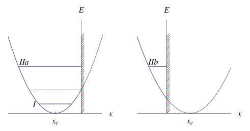
Figure 1: Harmonic oscillator potential $(x-x_{c})^{2}$ and a confining wall (edge) at $x=0$. Several regions in $(E,x_{c})$ parameter space have to be considered. For $x_{c}<0$, the low energy region ($I$) is defined by $E<x_{c}^{2}$, and the high energy region ($IIa$) is determined by $E>x_{c}^{2}$. For $x_{c}>0$, there is only a high energy region $IIb$ for which $E>x_{c}^{2}$. The crossover region is marked by the horizontal dashed line in the left panel.

The following definitions and notations will be used below in discussing some general features,

$$k(x)=\sqrt{E-v(x)}>0,\ \ \ (x_{1}\leq x\leq x_{2}),$$ (8a)

$${\cal S}(x,x^{\prime})\equiv\int_{x}^{x^{\prime}}k(t)dt,\ \ \ (x_{1}\leq x\leq x^{\prime}\leq x_{2}\leq 0),$$ (8b)

$$S(E,x_{c})={\cal S}(x_{1},x_{2}).$$ (8c)

The dependence of the WKB action $S(E,x_{c})$ on energy enters through that of the turning points as in equation (7). This action should satisfy a certain relation resulting from the WKB connection formulae at the turning points $x_{1}<x_{2}$. In most cases, the structure of this relation involves the action $S(E,x_{c})$ as an argument of a trigonometric function, and its decoding can then be casted in the general form,

$$S(E,x_{c})=\pi[n+\gamma(E,x_{c})].$$ (9)

It should be emphasized that equation (9) is not an identity, but, rather, an implicit equation for finding the eigenvalues $E_{n}(x_{c})$. The function $0\leq\gamma(E,x_{c})<1$ should be calculated independently and encodes the details of the connection formulae. Arriving at this equation (equivalently knowing $\gamma(E,x_{c})$ explicitly) is the central part of the WKB method (the computation of the action $S(E,x_{c})$ is straightforward in most cases). Once this task is achieved, the solutions $E_{n}(x_{c})$ of this implicit equation are the required eigenvalues within the WKB approximation. Inserting the solutions into equation (9) implies the identity

$$S(E_{n}(x_{c}),x_{c})=\pi[n+\gamma(E_{n}(x_{c}),x_{c})],$$ (10)

which defines $\gamma(E_{n}(x_{c}),x_{c})\equiv\gamma_{n}(x_{c})$ self consistently as function of the discrete energy quantum number $n$ and the continuous variable $x_{c}$.

The easier part of the WKB procedure is calculation of the action itself, which in the present problem of confined harmonic oscillator becomes elementary. It depends on the appropriate region in $(E,x_{c})$ parameter space, as depicted on figure 1. In the low energy region, $I$ the positions of the turning points are $x_{1}=x_{c}-\sqrt{E}$ and $x_{2}=x_{c}+\sqrt{E}$ and the action $S$ is given by

$$S=\int_{x_{c}-\sqrt{E}}^{x_{c}+\sqrt{E}}\sqrt{E-(x-x_{c})^{2}}dx={1\over 2}\pi E.$$ (11)

In both high energy region $IIa,IIb$, the turning points are located at $x_{1}=x_{c}-\sqrt{E}$ and $x_{2}=0$. The action is now dependent on $x_{c}$ and it is given by

$$S = \int_{x_{c}-\sqrt{E}}^{0}\sqrt{E-(x-x_{c})^{2}}dx$$ (12)

$$= {\pi E\over 4}-{E\over 2}\arcsin{x_{c}\over\sqrt{E}}-{x_{c}\over 2}\sqrt{E-x_{c}^{2}}.$$

The action has a dimension of energy and can be written as

$$S(E,x_{c})={\pi E\over 2}s(x_{c}/\sqrt{E}),$$ (13)

where the dimensionless function

$$s(t)={1\over 2}-{1\over\pi}\arcsin t-{t\over\pi}\sqrt{1-t^{2}}$$ (14)

has the following expansions

$$t\simeq\pm 1\qquad s(t)={1\mp 1\over 2}\pm{4\sqrt{2}\over 3\pi}(1-|t|)^{3/2}$$ (15a)

$$t\simeq 0\qquad s(t)={1\over 2}-{2t\over\pi}.$$ (15b)

The dependence of the action $S(E,x_{c})=\frac{\pi E}{2}s(t)$ on $t=x_{c}/\sqrt{E}$ is displayed in figure (2).

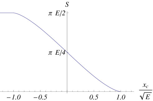
Figure 2: The action $S(E,x_{c})=\frac{\pi E}{2}s(t)$ as a function of $t=x_{c}/\sqrt{E}$ (with $E$ fixed). It varies between $\pi E/2$ for $t=-1\ \ (x_{c}\leq-\sqrt{E})$ and $0$ for $t=1\ \ (x_{c}\geq 0)$. For $t=x_{c}=0$, it is equal to $\pi E/4$.

The less trivial task which will occupy us in the next subsection is to calculate the function $\gamma(E,x_{c})$. When the potential is smooth and the wall is far from the right turning point $x_{2}$, $\gamma$ is determined by the standard WKB procedure such that the solutions for $x<x_{1}$ and $x>x_{2}$ (the classically forbidden regions) contain only decaying exponents. Each turning point $x_{i}$ then contributes a term $\frac{\beta_{i}}{4}$ where $\beta_{i}$ is an integer (also referred to as the Maslov index for the pertinent turning point), and $\gamma=\frac{1}{4}(\beta_{1}+\beta_{2})$. This is the situation appropriate in the lower part of region $I$ in figure 1 where $\beta_{1}=\beta_{2}=1$, implying $\gamma=\frac{1}{2}$. The definition can be extended to the situation when a turning point occurs at the wall. Although there is no solution to match on the right of the turning point, the condition $\psi(0)=0$ replaces the connection formula and implies $\beta_{\mbox{wall}}=2$. This is the situation relevant for the higher part of region $IIa$ and for region $IIb$ in figure 1, implying $\gamma=\frac{3}{4}$. As will be stressed below, the situation is different in the crossover region (around the horizontal dashed line in figure 1). Since $\gamma(E,x_{c})$ is expected to vary smoothly between $\frac{1}{2}$ and $\frac{3}{4}$, it cannot be written in terms of an integer $\beta_{2}$. If one insists on the same parametrization $\gamma=\frac{1}{4}(\beta_{1}+\beta_{2})$, this implies that $\beta_{2}$ is a non-integer Maslov index Friedrich . An attempt to use $\gamma=\frac{1}{2}$ for $E\leq x_{c}^{2}$ and $\gamma=\frac{3}{4}$ for $E\geq x_{c}^{2}$ is too naïve and leads to an artificial discontinuity at $E=x_{c}^{2}$ since

$$S(E=x_{c}^{2}+0,x_{c})=\frac{\pi E}{2}=\pi(n+\frac{3}{4})$$

$$\longrightarrow E_{n}(x_{c})=2n+\frac{3}{2},$$ (16a)

$$S(E=x_{c}^{2}-0,x_{c})=\frac{\pi E}{2}=\pi(n+\frac{3}{4})$$

$$\longrightarrow E_{n}(x_{c})=2n+1.$$ (16b)

This artificial discontinuity is displayed in figure 3 below.

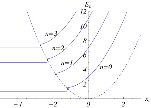
Figure 3: Energy eigenvalues $E_{n}(x_{c})$ obtained within the semiclassical approximation (9), where $S(E,x_{c})$ is given in equations (11,12) while $\gamma=\frac{1}{2}$ for $E<x_{c}^{2}$ and $\gamma=\frac{3}{4}$ for $E>x_{c}^{2}$. The (artificial) discontinuity occurring along the dashed line $E=x_{c}^{2}$ results from an improper treatment of the connection formula in the crossover region.

As will be explicitly demonstrated in the next section, the correct picture is indeed different: for fixed $n$, $\gamma_{n}(x_{c})$ is a monotonic and smooth function of $x_{c}$ which tends very quickly to $\frac{1}{2}$ at negative $x_{c}$ and to $\frac{3}{4}$ at $x_{c}\geq 0$.

III WKB evaluation of eigenvalues

A proper analysis of the crossover regions within the WKB formalism should then remedy the discontinuity problem by a proper treatment of the medium energy region $E\simeq x_{c}^{2}$. This is carried below by approaching the cross over region from below ($E\ll x_{c}^{2}\to E\approx x_{c}^{2}$) and from above ($E\gg x_{c}^{2}\to E\approx x_{c}^{2}$). The case $x_{c}\approx 0$ where the oscillator center is very close to the wall requires some special treatment at low energy where the linear approximation for the potential near the turning point is not valid. After this task is completed, the eigenvalues calculated by the WKB approach are compared with the exact ones, and the agreement is virtually perfect.

III.1 Approaching $E\approx x_{c}^{2}$ from below

When $E\leq x_{c}^{2}$ (region $I$ in figure (1)), the turning points and the WKB action are

$$x_{1,2}=x_{c}\pm\sqrt{E},$$ (17a)

$$S(E)=\frac{1}{2}\pi E.$$ (17b)

For $E\ll x_{c}^{2}$ the eigenvalues are expected to approach the energies $2n+1$ of the unrestricted harmonic oscillator. The question is how they are modified when $E$ approaches $x_{c}^{2}$ from below. For energies close to $x_{c}^{2}$ the turning point $x_{2}$ is rather close to the wall at $x=0$, and this must be taken into account. Practically, it means that the wave function in the classically forbidden region $x_{2}<x<0$ must include also an exponentially increasing contribution (beside the exponentially decreasing one), since vanishing of the wave function at the wall $x=0$ can be achieved only by a proper combination of the two waves. Therefore, a modification of the standard WKB connection procedure is required near $x_{2}$ in order to take into account the effect of the wall behind the turning point. On the other hand, the connecting procedure at the left turning point is standard. Recall that to the left of the point $x_{1}$ there is a single wave, that decays as $x\to-\infty$. This means that within the linear approximation for the potential near the turning points, only the first Airy function Ai is used near $x_{1}$. The connecting procedure around $x_{1}$ implies that the WKB approximation for the wave function for $x_{1}\leq x\leq x_{2}\leq 0$ is

$$\psi(x) = \frac{C}{\sqrt{k(x)}}\sin[{\cal S}(x_{1},x)+\frac{\pi}{4}]$$ (18)

$$= \frac{C}{\sqrt{k(x)}}\sin[S-{\cal S}(x,x_{2})+\frac{\pi}{4}],$$

where $C$ is a constant. The modification near the second turning point $x_{2}$ which is close to the wall assumes that in the small region $x_{2}<x<0$ the potential is approximated by a linear expansion near $x_{2}$ :

$$v(x)\approx E+2\sqrt{E}(x-x_{2}).$$ (19)

In terms of the variable

$$z=z(x)\equiv(4E)^{\frac{1}{6}}(x-x_{2}),$$ (20)

and within the approximation (19), the Schrödinger equation at the vicinity of $x_{2}$ reads

$$\frac{d^{2}\psi(z)}{dz^{2}}-z\psi(z)=0.$$ (21)

Unlike the analysis near $x_{1}$, here the combination of both Airy functions is required in order to construct the solution around $x_{2}$, that is,

$$\psi(z)=\alpha\mbox{Ai}(z)+\beta\mbox{Bi}(z).$$ (22)

When this combination is examined at $z<0$ (that is, $x<x_{2}$) and the asymptotic form of the Airy functions is used, it is found that the wave function at $x<x_{2}$ is,

$$\psi(x)=\alpha\sin[{\cal S}(x,x_{2})+\frac{\pi}{4}]+\beta\cos[{\cal S}(x,x_{2})+\frac{\pi}{4}].$$ (23)

Since this is the same function as that found in (18) we can compare the two and obtain a constraint on the coefficients $C,\alpha,\beta$. To this end, denote $\zeta\equiv{\cal S}(x,x_{2})+\frac{\pi}{4}$, and open the sine and cosine functions, to get

$$\sin\zeta(C\sin S+\alpha)+\cos\zeta(C\cos S+\beta)=0.$$ (24)

This holds for every $\zeta$, in the appropriate interval, hence each term in the bracket should vanish separately. This yields a couple of equations for the three coefficients $C,\alpha,\beta$. The wave function (22) should vanish at the wall $x=0$, that is ($z_{0}\equiv z(x=0)$) :

$$\psi(z_{0})=0,$$ (25a)

$$z_{0}=-(4E)^{\frac{1}{6}}x_{2}=-(4E)^{\frac{1}{6}}(x_{c}+\sqrt{E})>0,$$ (25b)

implying that

$$\beta=-\frac{\mbox{Ai}(z_{0})}{\mbox{Bi}(z_{0})}\alpha.$$ (26)

Employing the statement after equation (23) this leaves us with two homogeneous equations for $C$ and $\alpha$ :

$$C\sin S+\alpha=0,$$ (27a)

$$C\cos S-\frac{\mbox{Ai}(z_{0})}{\mbox{Bi}(z_{0})}\alpha=0,$$ (27b)

and the energies $E_{n}$ are obtained by requiring the vanishing of the determinant

$$\cos S+\frac{\mbox{Ai}(z_{0})}{\mbox{Bi}(z_{0})}\sin S=0.$$ (28)

The implicit dependence on the energy $E$ enters through the dependence of $S$ and $z_{0}$ on energy, equations (17b) and (25b) respectively. Equation (28) is recast in the WKB format as

$$S={\pi E\over 2}=\pi[n+\gamma(E,x_{c})]$$ (29)

where $0<\gamma<1$ is explicitly given by

$$\gamma(E,x_{c})=1-{1\over\pi}\arctan{\mbox{Bi}(z_{0})\over\mbox{Ai}(z_{0})},$$ (30)

with $z_{0}$ defined in (25b). The function $\gamma(E,x_{c})$ is plotted as function of the energy $E$ for several values of $x_{c}$ in figure 4.

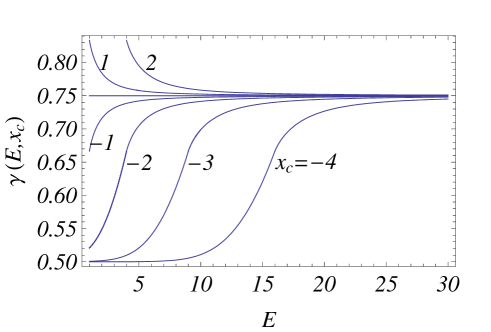
Figure 4: The function $\gamma(E,x_{c})$ defined in equation (30) is plotted versus $E$ for different values of $x_{c}=-4,-3,-2,-1,0,1,2$.

The eigenvalues $E_{n}(x_{c})$ are the intersection of the curves $\gamma(E,x_{c})$ (as function of $E$ with $x_{c}$ as a parameter) with the straight lines $\frac{1}{\pi}S(E,x_{c})-n$. In the two limiting cases $E\ll x_{c}^{2}$ and $E\approx x_{c}^{2}$ these solutions can be easily evaluated. When $E\ll x_{c}^{2}$, the value of $z_{0}$ is large. Then

$$\frac{\mbox{Ai}(z_{0})}{\mbox{Bi}(z_{0})}\approx\frac{1}{2}e^{-\frac{4}{3}z_{0}^{\frac{3}{2}}}\approx 0,$$ (31)

and equation (30) leads to the familiar result of the harmonic oscillator problem with $\gamma=1/2$ and $E_{n}=2n+1$. On the other hand, when the energy is very close to (but still lower than) $x_{c}^{2}$ then $z_{0}$ is very small, and hence,

$$\frac{\mbox{Ai}(z_{0})}{\mbox{Bi}(z_{0})}\approx\frac{\mbox{Ai}(0)}{\mbox{Bi}(0)}=\frac{1}{\sqrt{3}},$$ (32)

so that $\gamma=2/3$ and

$$E_{n}=2n+\frac{4}{3}.$$ (33)

This value $\gamma=\frac{2}{3}$ is intermediate between the ”high” and ”low” energy values $\frac{3}{4}$ and $\frac{1}{2}$. For $n=0$ this gives the energy $\frac{4}{3}$ instead of $\frac{3}{2}$ and $1$. The exact value is indeed $\frac{4}{3}$. The disagreement between the ”high energy” prediction $\frac{3}{2}$ and the exact value $\frac{4}{3}$ has been noticed for $n=0$ in table II of Ref.Vawter where it is dubbed as a WKB error. Our results show, however, that the WKB formalism as applied here is virtually exact.

III.2 Approaching $E\approx x_{c}^{2}$ from above

Consider now region (II) in figure 1, where $E\geq x_{c}^{2}$. In order to treat this ”high energy” region the linear expansion of $v(x)$, eq. (19) is now replaced by

$$v(x)\approx x_{c}^{2}-2x_{c}x,$$ (34)

so that the wave function satisfies the Schrödinger equation and the hard wall boundary conditions at $x=0$,

$$\psi^{\prime\prime}-(x_{c}^{2}-E-2xx_{c})\psi=0.$$ (35a)

$$\psi(0)=0.$$ (35b)

whose solution has the form

$$\psi(x)=\alpha\mbox{Ai}\left[{x_{c}^{2}-E-2xx_{c}\over|2x_{c}|^{2/3}}\right]+\beta\mbox{Bi}\left[{x_{c}^{2}-E-2xx_{c}\over|2x_{c}|^{2/3}}\right].$$ (36)

The hard wall condition at $x=0$ implies

$${\beta\over\alpha}=-\displaystyle{\mbox{Ai}\left[{x_{c}^{2}-E\over|2x_{c}|^{2/3}}\right]\over\mbox{Bi}\left[{x_{c}^{2}-E\over|2x_{c}|^{2/3}}\right]}\equiv-{\mbox{Ai}(-W)\over\mbox{Bi}(-W)},$$ (37)

where

$$W={E-x_{c}^{2}\over|2x_{c}|^{2/3}}>0.$$ (39)

At large distance $x<0$, the asymptotic form of the Airy functions for negative arguments can be used to yield

$$\psi(x) \propto \alpha\sin\left[{x_{c}^{2}-E-2xx_{c}\over|2x_{c}|^{2/3}}+{\pi\over 4}\right]$$ (40)

$$+ \beta\cos\left[{x_{c}^{2}-E-2xx_{c}\over|2x_{c}|^{2/3}}+{\pi\over 4}\right].$$

and the action for the linearized potential $v(x)$ is

$${\cal S}(x,0) = \int_{x}^{0}\sqrt{E-x_{c}^{2}+2xx_{c}}dx$$ (41)

$$= {(E-x_{c}^{2})^{3/2}\over 3x_{c}}-{(E-x_{c}^{2}+2xx_{c})^{3/2}\over 3x_{c}}.$$

Therefore the wavefunction has the form

$$\psi(x) \propto \alpha\sin\left[-\epsilon{\cal S}(x,0)+\delta+{\pi\over 4}\right]$$ (42)

$$+ \beta\cos\left[-\epsilon{\cal S}(x,0)+\delta+{\pi\over 4}\right],$$

with

$$\epsilon=\mbox{sign}(x_{c}),$$ (43a)

$$\delta={(E-x_{c}^{2})^{3/2}\over 3|x_{c}|}={2\over 3}W^{3/2}.$$ (43b)

On the other hand, following the procedure leading to equation (18) the wave function resulting from the connecting formula at $x=x_{1}$ is ($x_{1}\leq x\leq 0$)

$$\psi(x) = \frac{C}{\sqrt{k(x)}}\sin[S-{\cal S}(x,0)+\frac{\pi}{4}]$$ (44)

$$= \frac{C}{\sqrt{k(x)}}\cos[{\cal S}(x,0)+\frac{\pi}{4}-S].$$

It is now allowed to compare the two expressions (42) and (44) for the same wave function. These two expressions should be equal for any value of the variable ${\cal S}(x,0)$. Equating the coefficients of $\sin{\cal S}(x,0)$ and $\cos{\cal S}(x,0)$ to $0$ (each one separately), and employing the relation (37) then result in the following two equations for $C$ and $\alpha$ :

$$-\alpha\epsilon\cos(\delta+{\pi\over 4})+\beta\epsilon\sin(\delta+{\pi\over 4}) = -C\cos(S+{\pi\over 4}),$$

$$\alpha\sin(\delta+{\pi\over 4})+\beta\cos(\delta+{\pi\over 4}) = C\sin(S+{\pi\over 4}),$$ (45a)

leading to

$$\tan(S+{\pi\over 4})=\epsilon\cot(\delta_{0}-\delta+{\pi\over 4})$$ (46)

with

$$\tan\delta_{0}={\alpha\over\beta}=-{\mbox{Bi}(-W)\over\mbox{Ai}(-W)}.$$ (47)

Finally, the energy levels $E(x_{c})$ are given by the action (12) and

$$\tan(S+{\pi\over 4})=-\epsilon\cot\left(\arctan{\mbox{Bi}[-W]\over\mbox{Ai}[-W]}+{2\over 3}W^{3/2}+{\pi\over 4}\right)$$

or, equivalently, by the central expression,

$$S(E,x_{c})=\pi[n+\gamma(E,x_{c})]$$ (49)

where $0<\gamma(E,x_{c})<1$ is given explicitly by (compare with equation (30) applicable for the case $E\leq x_{c}^{2}$),

$$\gamma(E,x_{c})={3\over 4}$$

$$-{\epsilon\over\pi}\arctan\cot\left(\arctan\frac{\mbox{Bi}}{\mbox{Ai}}+\frac{2}{3}W^{\frac{3}{2}}+\frac{\pi}{4}\right)$$ (50)

This function, calculated here for $x_{c}>-\sqrt{E}$ is shown on figure (4). It has simple values in the following special cases :

$$x_{c}=-\sqrt{E},\quad W=0,\quad\gamma(E,x_{c})=2/3,\quad E_{n}=2n+{4\over 3},$$ (51a)

$$x_{c}=0,\quad W=\infty,\quad\gamma(E,x_{c})=3/4,\quad E_{n}=4n+3.$$ (51b)

III.3 Perturbation expansion for small $|x_{c}|$

Near $x_{c}=0$ and at low energy the linear approximation is not justified because at $x_{c}=0$ the linear term vanishes. It is then necessary to modify the semiclassical formalism for evaluating $E_{n}(x_{c})$ and $\gamma_{n}(x_{c})$ near $x_{c}=0$. Here a simple perturbative expansion for small $x_{c}$ is used. The unperturbed hamiltonian is,

$$H_{0}=p^{2}+x^{2}$$ (52)

The solutions $\psi_{n}(x)$ with $\psi(0)=0$ are the antisymmetric eigenfunctions of the free harmonic oscillator (with energy $E_{n}=4n+3$),

$$\psi_{n}(x)={e^{-x^{2}/2}H_{2n+1}(x)\over\sqrt{\pi 2^{2n}(2n+1)!}}.$$ (53)

where $H_{n}$ are the Hermite polinomyals. The perturbation term for small $x_{c}$ is $-2xx_{c}$, and the first order correction then yields the perturbed energies,

$$E_{n}(x_{c}) \approx 4n+3-2x_{c}\int_{-\infty}^{0}x\psi_{n}^{2}(x)dx$$ (54)

$$= (4n+3)+{4x_{c}\over\sqrt{\pi}}\displaystyle\prod_{1}^{n}\left(1+{1\over 2p}\right)$$

The value of $\gamma_{c}(x_{c})$ near $x_{c}=0$ can therefore be obtained from the quantization condition eq. (10). Expanding the action $S(E,x_{c})$ near $x_{c}=0$ to first order in $x_{c}$ reads $S(E,x_{c})=\pi E/4-\sqrt{E}x_{c}$, which implies,

$$\gamma_{n}(x_{c})={3\over 4}+\beta_{n}x_{c}.$$ (55)

The coefficients $\beta_{n}$ are given by,

$$\beta_{n} = {1\over\sqrt{\pi}}\displaystyle\prod_{1}^{n}\left(1+{1\over 2p}\right)-{\sqrt{4n+3}\over\pi}$$

$$\beta_{0} = 0.01286$$

$$\beta_{1} = 0.00416$$

$$\beta_{2} = 0.00214$$

$$\beta_{3} = 0.00135$$ (56)

In the limit $n\rightarrow\infty$, the product tends to $\sqrt{{4n+3\over\pi}}$, so that $\beta_{\infty}=0$. Equation (55) shows that at low energy and for $x_{c}$ very close to $0$ (when the linear approximation to the potential fails), $\gamma_{n}(x_{c})$ shoots up slightly above $\frac{3}{4}$. Since $\beta_{n}$ is small, the deviation $\beta_{n}x_{c}$ is virtually negligible.

III.4 Comparing WKB results with the exact ones

The central result of the foregoing discussion can now be presented. Once the function $\gamma(E,x_{c})$ is known, the spectrum $E_{n}(x_{c})$ is entirely determined by the implicit equation (9 ). This is calculated and displayed as solid lines in figure (5). The exact eigenvalues are marked by dots on the same figure. The fit is indeed perfect.

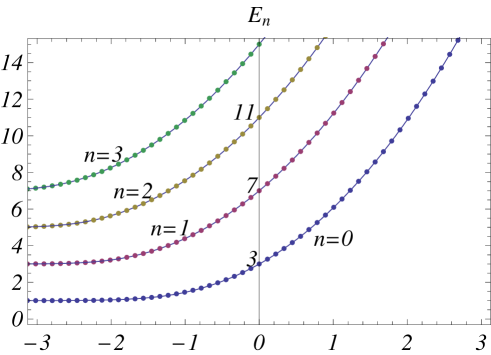
Figure 5: The solid lines display the energy levels $E_{n}(x_{c})$ calculated in the WKB approximation as function of the continuous parameter $x_{c}$ . The exact eigenvalues (obtained by numerical diagonalization) are represented by the full circles.

IV Inspecting scaling behavior

After substantiating the efficiency of the WKB method for the confined harmonic oscillator problem (summarized in figure 5), and elucidating the functional form of $\gamma(E,x_{c})$ (see equations (30,50)) let us return to the question of scaling posed in the Introduction. It should be stressed that the notion of scaling here simply means that some functions of $x_{c}$ and $n$ can be represented as functions of a certain combination of these two variables. It has nothing to do with thermodynamics, of course, although the variable $n$ is, in some sense, analogous to the notion of length scale.

IV.1 Scaling of $\gamma_{n}(x_{c})$

Before discussing the scaling of the energies themselves it is useful to check a possible scaling behavior of $\gamma_{n}(x_{c})$.

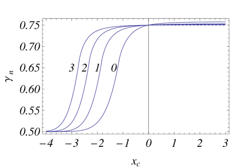
Figure 6: The function $\gamma_{n}(x_{c})$ as function of $x_{c}$ for $n=0,1,2,3$. Its calculation is explained at the beginning of this subsection.

To obtain this function explicitly the eigenvalues $E_{n}(x_{c})$ are calculated as explained in the previous section, and then substituted instead of $E$ in the function $\gamma(E,x_{c})$ defined in equations (30,50)) leading to the desired function $\gamma_{n}(x_{c})=\gamma[E_{n}(x_{c}),x_{c}]$. It is displayed as function of $x_{c}$ for several values of $n$ in figure (6). Looking at figure 6 one is tempted to search for a ”scaling relation” in the sense that $\gamma_{n}(x_{c})$ depends on a certain combination $X(n,x_{c})$ of $x_{c}$ and $n$. Such combination can then be used as a scaling variable where all the curves collapse on a single one. Based on our previous analysis it is established that $\gamma_{n}(x_{c})$ and the spectrum $E_{n}(x_{c})$ is very well fitted (within 2 %) by the function

$$\gamma_{n}(x_{c}) = 1$$

$$- {1\over\pi}\arctan{\mbox{Bi}[-2^{1/3}(2n+{4\over 3})^{1/6}(x_{c}+\sqrt{2n+{4\over 3}})]\over\mbox{Ai}[-2^{1/3}(2n+{4\over 3})^{1/6}(x_{c}+\sqrt{2n+{4\over 3}})]}$$

for $x_{c}<-\sqrt{2n+{4\over 3}}$, and by the function

$$\gamma_{n}(x_{c})=1-{1\over\pi}\arctan\tan\left(\arctan{\mbox{Bi}[-W_{n}]\over\mbox{Ai}[-W_{n}]}+{2\over 3}W_{n}^{3/2}\right),$$

$$\mbox{with}\qquad W_{n}(x_{c})={2n+{4\over 3}-x_{c}^{2}|2x_{c}|^{2/3}},$$ (58)

for $-\sqrt{2n+{4\over 3}}<x_{c}<0$ and by $\gamma_{n}(x_{c})=3/4$ for $x_{c}<0$.

Strictly speaking then, there is no single combination of $n$ and $x_{c}$ that enters both expressions. Practically, however, when the variable $X=(2n+{4\over 3})^{1/6}(x_{c}+\sqrt{2n+{4\over 3}})$ is used, the collapse of all curves is very good as can be seen in figure 7 where $\gamma_{n}(x_{c})=\gamma(X)$, is plotted against $X$.

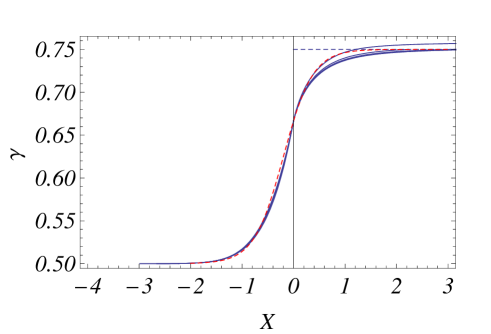
Figure 7: The functions $\gamma_{n}(x_{c})$ are plotted as a function of the scaling variable $X=(2n+{4\over 3})^{1/6}(x_{c}+\sqrt{2n+{4\over 3}})$. The dashed line is the function $\gamma(X)$ defined by equation (59).

Moreover, $\gamma(X)$ is very accurately fitted by the function

$$\gamma(X)={3\over 4}-{1\over 4}{1\over 2\exp AX+1}$$ (59)

where $A\simeq 3.5$, represented by the dashed line in figure 7. The energies $E_{n}(x_{c})$ are then calculable (within 2 % accuracy) through the solution of the standard WKB implicit equation,

$$S(E_{n},x_{c})=\pi[n+\gamma(X)]$$ (60)

with $\gamma(X)$ as given by the approximate formula (59).

IV.2 Scaling of edge state energies $E_{n}(x_{c})$

Turning now to the possible scaling of edge state energies, consider the identity (10) and suppose, for the moment that $\gamma_{n}(x_{c})$ is a constant. After dividing both sides by $2\pi(n+\gamma)$ and defining the scaling variables

$$y=x_{c}/2\sqrt{n+\gamma},$$ (61a)

$$u=E/4(n+\gamma),$$ (61b)

the identity (10) takes the form

$$\frac{1-u}{2}+\frac{u}{\pi}\arcsin\frac{y}{\sqrt{u}}+\frac{y}{\pi}\sqrt{u-y^{2}}=0.$$ (62)

Equation (62) then implicitly defines the functional relation

$$u=\frac{E_{n}}{4(n+\gamma)}=f(y)=f(\frac{x_{c}}{2\sqrt{n+\gamma}}),$$ (63)

between $u$ and $y$. The function $f(y)$ is shown in figure 8 below.

Figure 8: Universal function $f(y)$ and $y^{2}$ (dashed line).

From the expansions (15b) of the function $s(t)$, it is easy to deduce that the function $f(y)$, shown on figure (8), has the following limits

$$y\leq-1/\sqrt{2}\ \ f(y)={1\over 2},$$

$$0>y\geq-1/\sqrt{2}\ \ f(y)={1\over 2}+{4\ 2^{1/4}\over 3\pi}({1\over\sqrt{2}}+y)^{3/2},$$

$$y\simeq 0\ \ f(y)=1+{4y\over\pi},$$

$$y\rightarrow\infty\ \ f(y)=y^{2}+{1\over 2}\left({3\pi\over\sqrt{2}}\right)^{2/3}y^{4/3}.$$ (64)

However, the relation (62) is of little use, because $\gamma$ is not known in advance and its evaluation is part of the problem. A more practical approach would then be to fix an appropriate constant value $\gamma_{0}$ and take account of the small variation of $\frac{1}{2}\leq\gamma\leq\frac{3}{4}$ by some correction. From the edge-state point of view, the region $x_{c}>-1$ for which $\gamma\approx\frac{3}{4}\equiv\gamma_{0}$ is the most relevant one. Therefore, the ”length scale” is fixed as $L_{n}=4(n+\gamma_{0})=4n+3$ and expand equation (63) to first order around $\gamma_{0}$. To save notations $u$ and $y$ are now defined with $\gamma=\gamma_{0}=3/4$. The result is

$$\frac{E_{n}}{4n+3}=u=f(y)\left\{1-\frac{3-4\gamma}{4n+3}\left[1-\frac{yf^{\prime}(y)}{2f(y)}\right]\right\}.$$ (65)

Strictly speaking, the problem mentioned in connection with equation (62) still remains, but this time it is casted in a form showing that exact scaling is expected to work for large $n$ as $L_{n}=4n+3\to\infty$. The second term in the square brackets can be neglected because for large $y$ $\gamma=3/4$ and the correction disappears, whereas for small $y$, $f(y)\to 1/2$ so its derivative vanishes. It is then reasonable to suggest the following relation

$$\frac{E_{n}(x_{c})}{4[n+\gamma_{n}(x_{c})]}=f(y),$$ (66)

where, employing the expression (59) for $\gamma_{n}(x_{c})$,

$$4[n+\gamma_{n}(x_{c})]=4n+3-\frac{1}{2e^{AX_{n}(x_{c})}+1},$$ (67)

$$\mbox{with}\ \ \ X_{n}(x_{c})=(2n+{4\over 3})^{1/6}\left[x_{c}+(2n+{4\over 3})^{\frac{1}{2}}\right],$$

with $A=\simeq 3.5$. To test the scaling relation, the exact eigenvalues $E_{n}(x_{c})$ for $n=0,1,\ldots 13$ were calculated via numerical diagonalization resulting in $14$ curves each contains $100$ points $x_{c}$ (we have already shown that these energies can also be calculated within the WKB formalism developed here).

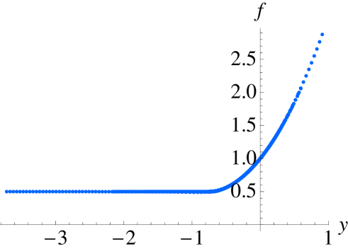
Figure 9: Test of the scaling relation (66). The numbers $E_{n}(x_{c})$ are obtained numerically by exact diagonalization and the function $\gamma(x_{c})$ is approximated employing equation (67). The numbers appearing on the LHS of equation (66) are then displayed as function of the scaling variable $y=\frac{x_{c}}{\sqrt{4n+3}}$, thus generating a smooth curve representing the scaling function $f(y)$ given by eqs. (62,63). It results from the collapse of $14$ curves $E_{n}(x_{c})$ with $n=0,1,\dots 13$, each contains $100$ points $x_{c}$.

The $1400$ numbers appearing on the LHS of equation (66) are thus computed and displayed against the scaling variable $y$ in figure 9 below. The smooth curve gives the scaling function $f(y)$ and for $y>-\frac{1}{\sqrt{2}}$ it coincides with the curve of figure 8. The collapse of $14$ curves on a single one is remarkable. The upshot is that equation (66) with $f(y)$ analyzed in equations (64) and $\gamma(x_{c})$ parametrized as in equation (59) is an excellent approximation for $E_{n}(x_{c})$.

Acknowledgment
We would like to thank Jean Marc Luck and Benoit Douçot for invaluable help and suggestions.

References

- (1) B. I. Halperin, Phys. Rev. B (1982).
- (2) A. H. Macdonald and P. Streda, Phys. Rev. B29, 1616 (1984).
- (3) M. Büttiker, Phys. Rev. B (1988).
- (4) C. Kane and E. J. Mele, Phys. Rev. Lett. (2005).
- (5) H. E. Montgomery Jr, G. Campoy and N. Aquino, arXiv:0803.4029 (Refs. 17-39 therein), (2008).
- (6) M. Abramowitz and Irene A. Stegun, Hanbook of Mathematical Functions, National Bureau of Standards, Applied Mathematic Series (1964). See Chapter 19, Parabolic Cylinder Functions.
- (7) R. Vawter, Phys. Rev. 174, 749 (1968).
- (8) D. S. Krähmer, W. P. Schleich and V. P. Yakovlev, J. Phys. A: Math. Gen. 31, 4493 (1998).
- (9) A. Sinha and R. Ryochudhury, Int. Jour. of Quantum Chemistry, 73, Issue 6, 497 (1999).
- (10) U. Larsen, J. Phys. A: Math. Gen. 16, 2137 (1983).
- (11) G. A. Arteca, S. A. Maluendes, F. M. Fernandez, E. A. Castro, Int. Jour. of Quantum Chemistry, 24, Issue 2, 497 (1983).
- (12) A. Isihara and K. Ebina, J. Phys. C: Solid State Physics, 21, L1079 (1988).
- (13) G. Campoy, N. Aquino and V. D. Granados, J. Phys. A: Math. Gen. 35, 4903 (2002).
- (14) A. K. Ghatak, I. C. Goyal, R. Jindal and Y. P. Varshni, Can. J. Phys. 76(5), 351 (1998).
- (15) H. Friedrich and J. Trost, Phys. Rev. A54, 1136 (1996).