Numerical simulation of excitation and propagation of helioseismic MHD waves: Effects of inclined magnetic field

Abstract

Investigation of propagation, conversion, and scattering of MHD waves in the Sun is very important for understanding the mechanisms of observed oscillations and waves in sunspots and active regions. We have developed 3D linear MHD numerical model to investigate influence of the magnetic field on excitation and properties of the MHD waves. The results show that the magnetic field can substantially change the properties of the surface gravity waves ($f$-mode), but their influence on the acoustic-type waves ($p$-modes) is rather moderate. Comparison our simulations with the time-distance helioseismology results from SOHO/MDI shows that the travel time variations caused by the inclined magnetic field do not exceed 25% of the observed amplitude even for strong fields of 1400–1900 G. This can be an indication that other effects (e.g. background flows and non-uniform distribution of magnetic field) can contribute to the observed travel time variations. The travel time variations caused by the wave interaction with magnetic field are in phase with the observations for strong fields of 1400–1900 G if Doppler velocities are taken at the height of 300 km above the photosphere where plasma parameter $\beta\ll 1$. The simulations show that the travel times only weakly depend on the height of velocity observation. For the photospheric level the travel times are systematically smaller on approximately 0.12 min then for the hight of 300 km above the photosphere for all studied ranges of the magnetic field strength and inclination angles. The numerical MHD wave modeling and new data from the HMI instrument of the Solar Dynamics Observatory will substantially advance our knowledge of the wave interaction with strong magnetic fields on the Sun and improve the local helioseismology diagnostics.

1 Introduction

Local helioseismology has provided important results about the structures and dynamics of the solar plasma below the visible surface of the Sun, associated with sunspots and active regions (e.g. Duvall et al., 1996; Kosovichev, 1996; Kosovichev et al., 2000; Zhao et al., 2001; Haber et al., 2000; Komm et al., 2008). The helioseismic inferences help us to understand the complicated processes of the origin solar magnetic structures, formation and evolution of sunspots and active regions. These studies are based on measurements and inversions of variations of acoustic travel times and oscillation frequencies in the areas occupied by magnetic field and around them.

There are several factors that may cause the observed variations of the oscillation properties, and it is very important to painstakingly investigate their effects for improving the reliability of the helioseismic inference (Bogdan, 2000). Such studies are carried out both observationally by doing various experiments with the data analysis procedure, e.g. by masking the regions of strong field, doing ”double-skip” experiments etc. (e.g. Zhao & Kosovichev, 2006), and theoretically by simulating wave propagation in various conditions of the solar convection zone and calculating how these conditions affect the helioseismic observables, such as the oscillation power spectrum and acoustic travel times (Georgobiani et al., 2007; Zhao et al., 2007). We emphasize that for correct interpretation of helioseismic results the theoretical modeling must include calculations of the actual observables, taking into account all important aspects of the data measurement procedure, such as data filtering and averaging, and geometrical factors (Nigam et al., 2007). Unfortunately, in many theoretical studies the actual helioseismic measurement procedure is not modeled, and this may lead to incorrect conclusions about the role of various factors in the helioseismic results.

In general, the main factors causing variations in helioseismic travel times in solar magnetic regions, can be divided in two types: direct and indirect. The direct effects are due to the additional magnetic restoring force, which changes the wave speed and may transform acoustic waves into different types of MHD waves. The indirect effects are due to the changes in the convective and thermodynamic properties in magnetic regions. These include depth-dependent variations of temperature and density, large-scale flows and changes in wave source distribution and strength. Both direct and indirect effects may be present in the observed travel-time and frequency variations and cannot be easily disentangled by data analyses causing confusions and misinterpretations. Thus, it is very important to investigate the various aspects by numerically modeling the individual factors separately.

In particular, we have investigated the effects of the suppressed excitation of acoustic waves in sunspot regions, where strong magnetic field inhibits convective motions, which are the primary source of solar waves (Parchevsky & Kosovichev, 2007a). The results showed that the suppression of acoustic sources may explain most of the observed deficit of acoustic power in sunspot regions (Parchevsky & Kosovichev, 2007b), and also cause systematic shifts in the travel-time measurements. However, these shifts are significantly smaller than the observed variations of the travel times and and also have the opposite sign (Parchevsky et al., 2008), and, thus, cannot affect the basic conclusions on the sunspot sound-speed structure, contrary to previous suggestions (e.g. Rajaguru et al., 2006).

The goal of this paper is to model the excitation and propagation of helioseismic waves (both f- and p-modes) in the presence of inclined magnetic field and investigate the importance of the inclined field in the time-distance helioseismology measurements by carefully modeling the measurement procedure and comparing with the observational results, obtained by Zhao & Kosovichev (2006). The issue of the influence of the inclined magnetic field was raised by Schunker et al. (2005), who found that the phase shift of the signal in the penumbra of a sunspot, measured by the acoustic holography technique varies with the sunspot position on the disk. They attributed this to the variations of the angle between the inclined magnetic field of the penumbra and the line-of-sight. They suggested that the variations of the phase shift may affect the inferences of the sound-speed distribution below sunspots, inferred by time-distance helioseismology. However, Zhao & Kosovichev (2006) repeated the analysis of the same sunspot by the time-distance technique, and found substantially smaller variations with the position on the disk, and no significant effect on the wave-speed profile. They also found that the variations due to the inclination angle exist only for the wave measurements using the Doppler-shift signal, and that the variations are absent when the travel times are measured from the simultaneous intensity observations from SOHO/MDI. This result indicates that the observed variations with the inclination angle of the Doppler-shift measurements are likely to be related to changes of the ratio between the vertical and horizontal components of the displacement vector of the solar oscillations in the penumbra, and not the wave transformation or other effects, which could affect the modal structure of the oscillations. The solar oscillation theory predicts that the ratio between the vertical and horizontal components mostly depends on the surface boundary conditions (e.g. Unno et al., 1989). In the sunspot umbra, the boundary conditions may change due to the inclined magnetic field or/and near surface flows, the Evershed effect, which is observed directly in the Doppler-shift data and shows a significant center-to-limb variation.

In this paper, we present the results of numerical modeling of the inclined magnetic field on the time-distance helioseismology measurements by isolating this affect in a simple magnetic configuration, and show that only 25% of travel time variations measured by Zhao & Kosovichev (2006) can be explained by a direct influence of the inclined magnetic field on acoustic waves. In Sec. 2, we present the governing equation and describe the numerical method of 3D modeling of helioseismic MHD waves. In Sec. 3, we present the code verification results comparing the numerical results with analytical solutions for simple cases. In Sec. 4, we present the simulation results of the wave propagation in regions with inclined magnetic field, calculation of the center-to-limb variations of the time-distance helioseismology measurements and comparison with the observational results.

2 Numerical Model

2.1 Governing equations and numerical scheme

Propagation of MHD waves inside the Sun in the presence of magnetic field is described by the following system of linearized MHD equations:

$$\begin{array}[]{l}\displaystyle\frac{\partial\rho^{\prime}}{\partial t}+\nabla\cdot\mbox{\boldmath$m$}^{\prime}=0,\\[12.0pt] \displaystyle\frac{\partial\mbox{\boldmath$m$}^{\prime}}{\partial t}+\nabla p^{\prime}-\frac{1}{4\pi\rho_{0}}[(\nabla\times\mbox{\boldmath$B$}_{0})\times\mbox{\boldmath$B$}^{\prime}+(\nabla\times\mbox{\boldmath$B$}^{\prime})\times\mbox{\boldmath$B$}_{0}]=\mbox{\boldmath$g$}_{0}\rho^{\prime}+\mbox{\boldmath$S$},\\[12.0pt] \displaystyle\frac{\partial p^{\prime}}{\partial t}+c_{s0}^{2}\nabla\cdot\mbox{\boldmath$m$}^{\prime}+c_{s0}^{2}\frac{\mathcal{N}^{\,2}_{0}}{g_{0}}m_{z}=0,\end{array}$$ (1)

where $\mbox{\boldmath$m$}^{\prime}=\rho_{0}\mbox{\boldmath$v$}^{\prime}$ is the momentum perturbation, $\mbox{\boldmath$v$}^{\prime}$, $\rho^{\prime}$, $p^{\prime}$, and $\mbox{\boldmath$B$}^{\prime}$ are the velocity, density, pressure, and magnetic field perturbations respectively, $S$ is the wave source function. The quantities with subscript 0, such as gravity $\mbox{\boldmath$g$}_{0}$, sound speed $c_{s0}$, and Brünt-Väisälä frequency $\mathcal{N}_{0}$ correspond to the background model. The spatial and temporal behavior of the wave source is modeled by function $f(x,y,z,t)$:

$$f(x,y,z,t)=\left\{\begin{array}[]{ll}\displaystyle A\left[1-\frac{r^{2}}{R_{src}^{2}}\right]^{2}\left(1-2\tau^{2}\right)e^{-\tau^{2}}&\mbox{if }r\leq R_{src}\\ \displaystyle 0&\mbox{if }r>R_{src},\end{array}\right.$$ (2)

where $R_{src}$ is the source radius, $r=\sqrt{(x-x_{src})^{2}+(y-y_{src})^{2}+(z-z_{src})^{2}}$ is the distance from the source center, $\tau$ is given by equation

$$\tau=\frac{\omega(t-t_{0})}{2}-\pi,\qquad t_{0}\leq t\leq t_{0}+\frac{4\pi}{\omega},$$ (3)

where $\omega$ is the central source frequency, $t_{0}$ is the moment of the source initiation. In our simulations we used sources of two types: source of vertical force $\mbox{\boldmath$S$}=(0,0,f)^{T}$ and pressure source $\mbox{\boldmath$S$}=\nabla f$. Superposition of such randomly distributed sources describes very well the observed solar oscillation spectrum (Parchevsky & Kosovichev, 2007a).

For numerical solution of equations (1) a semi-discrete finite difference scheme of high order was used. At the top and bottom boundaries non-reflective boundary conditions based on the perfectly matched layer (PML) technique were set. We used the standard solar model S (Christensen-Dalsgaard et al., 1996) with a smoothly joined model of the chromosphere of Vernazza et al. (1976), as the background model. The background model was modified near the photosphere to make it convectively stable. Details of numerical realization of the code and the background model can be found in Parchevsky & Kosovichev (2007a).

2.2 Code verification for different types of MHD waves

To verify the code and estimate the total error of the method we compare numerical results with simple analytical solutions. We assume that all quantities depend on time $t$ and one spatial coordinate $x$ only, and consider the following linearized adiabatic 1D system of the MHD equations in Cartesian coordinates for a uniform background model

$$\begin{array}[]{l}\displaystyle\frac{\partial\rho}{\partial t}+\bar{\rho}\frac{\partial u}{\partial x}=0,\\[12.0pt] \displaystyle\frac{\partial u}{\partial t}+\frac{1}{\bar{\rho}}\frac{\partial p}{\partial x}+\frac{\bar{B}_{z}}{4\pi\bar{\rho}}\frac{\partial B_{z}}{\partial z}=0,\\[12.0pt] \displaystyle\frac{\partial v}{\partial t}-\frac{\bar{B}_{x}}{4\pi\bar{\rho}}\frac{\partial B_{y}}{\partial x}=0,\\[12.0pt] \displaystyle\frac{\partial w}{\partial t}-\frac{\bar{B}_{x}}{4\pi\bar{\rho}}\frac{\partial B_{z}}{\partial x}=0,\\[12.0pt] \displaystyle\frac{\partial B_{y}}{\partial t}-\bar{B}_{x}\frac{\partial v}{\partial x}=0,\\[12.0pt] \displaystyle\frac{\partial B_{z}}{\partial t}+\bar{B}_{z}\frac{\partial u}{\partial x}-\bar{B}_{x}\frac{\partial w}{\partial x}=0,\\[12.0pt] \displaystyle\frac{\partial p}{\partial t}+\bar{c}_{s}^{2}\bar{\rho}\frac{\partial u}{\partial x}=0,\end{array}$$ (4)

where $\bar{c}_{s}$ is the sound speed in the background model, $p$, $\rho$ are the pressure and density, $u$, $v$, and $w$ are the velocity components, $B_{x}$, $B_{y}$, $B_{z}$ are the components of the magnetic field respectively. The quantities related to the background model are marked here by overbar. By rotating of the coordinate frame around OZ axis we set $\bar{B}_{y}=0$. Equations (4) can be rewritten in matrix notations

$$\begin{array}[]{l}\displaystyle\frac{\partial\mbox{\boldmath$U$}}{\partial t}+\mbox{\boldmath$A$}\frac{\partial\mbox{\boldmath$U$}}{\partial x}=0,\end{array}$$ (5)

where $\mbox{\boldmath$U$}=(\rho,u,v,w,B_{y},B_{z},p)^{T}$. We seek a solution of equations (5) in infinite interval $-\infty<x<\infty$ in the form of plane waves

$$\mbox{\boldmath$U$}=\hat{\mbox{\boldmath$U$}}\exp\left[i(kx-\omega t)\right]$$ (6)

Substituting equation (6) into system (5) we obtain an eigenvalue problem for amplitude $\hat{\mbox{\boldmath$U$}}$

$$\mbox{\boldmath$A$}\hat{\mbox{\boldmath$U$}}=\frac{\omega}{k}\hat{\mbox{\boldmath$U$}},$$ (7)

where $V=\omega/k$ is the phase speed of the wave. Thus, the amplitudes of various MHD quantities are the components of eigenvectors of matrix $A$, and eigenvalues of this matrix represent phase velocities of the corresponded waves. From this we calculate the amplitudes of the entropy, Alfven, slow, and fast MHD waves:

$$\begin{array}[]{ccccccc}\hat{\mbox{\boldmath$U$}}_{s}=(\bar{\rho},&0,&0,&0,&0,&0,&0)^{T}\\[5.0pt] \hat{\mbox{\boldmath$U$}}_{\mp A}=(0,&0,&\pm V_{A},&0,&\bar{B}_{x},&0,&0)^{T}\\[5.0pt] \hat{\mbox{\boldmath$U$}}_{\mp S}=(\bar{\rho},&\mp V_{S},&0,&\displaystyle\mp\frac{c_{A}^{2}V_{S}\sin\theta\cos\theta}{V_{A}^{2}-V_{S}^{2}},&0,&\displaystyle-\frac{B_{0}V_{S}^{2}\sin\theta}{V_{A}^{2}-V_{S}^{2}},&c_{s}^{2}\bar{\rho})^{T}\\[12.0pt] \hat{\mbox{\boldmath$U$}}_{\mp F}=(\bar{\rho},&\mp V_{F},&0,&\displaystyle\mp\frac{c_{A}^{2}V_{F}\sin\theta\cos\theta}{V_{A}^{2}-V_{F}^{2}},&0,&\displaystyle-\frac{B_{0}V_{F}^{2}\sin\theta}{V_{A}^{2}-V_{F}^{2}},&c_{s}^{2}\bar{\rho})^{T}.\end{array}$$ (8)

The phase velocities of these waves are $0$, $\mp V_{A}$, $\mp V_{S}$, and $\mp V_{F}$ respectively, where

$$\begin{array}[]{l}V_{A}=c_{A}\cos\theta,\\ \displaystyle V_{S}=\frac{1}{\sqrt{2}}\sqrt{c_{s}^{2}+c_{A}^{2}-\sqrt{c_{s}^{4}+c_{A}^{4}-2c_{s}^{2}c_{A}^{2}\cos 2\theta}},\\[12.0pt] \displaystyle V_{F}=\frac{1}{\sqrt{2}}\sqrt{c_{s}^{2}+c_{A}^{2}+\sqrt{c_{s}^{4}+c_{A}^{4}-2c_{s}^{2}c_{A}^{2}\cos 2\theta}}.\end{array}$$ (9)

Here $c_{A}=\bar{B}/\sqrt{4\pi\bar{\rho}}$ is the Alfven speed, $\theta$ is the angle between the wave vector and the background magnetic field ($\bar{B}_{x}=\bar{B}\cos\theta,\;\bar{B}_{z}=\bar{B}\sin\theta$). Equations (6), (8), and (9) give us an analytical solution to 1D system of MHD equations (4), which includes all types of MHD waves. Initial conditions for these waves are obtained by setting $t=0$ in equation (6).

For testing the numerical simulations we use our 3D code with initial conditions depending only on $x$ variable. The calculations are carried out in the Cartesian geometry in the domain of 15.46 Mm$\times$15.46 Mm$\times$3.05 Mm with the numbers of grid points: $N_{x}=N_{y}=104,\;N_{z}=71$. All boundary conditions are chosen periodic simulating an infinite spatial domain. Wave vector $k=10\pi/(N_{x}+1)\Delta x$ is chosen in a way to match the periodic boundary conditions. In dimensionless variables $\tilde{\rho}=\rho/\bar{\rho}$, $\tilde{p}=p/\bar{\rho}\bar{c}_{s}^{2}$, $\tilde{\mbox{\boldmath$v$}}=\mbox{\boldmath$v$}/\bar{c}_{s}$, and $\tilde{B}^{2}=B^{2}/4\pi\bar{\rho}\bar{c}_{s}^{2}$ parameters of the background model are

$$\bar{\rho}=1,\quad\bar{c}_{s}=1,\quad\bar{B}=0.5,\quad c_{A}=0.5,\quad\theta=\pi/4.$$ (10)

The amplitude of the Alfven wave (in chosen dimensionless variables) traveling in the positive direction of the $x$-axis is $\hat{\mbox{\boldmath$U$}}_{+A}=(0,\>0,\>-1,\>0,\>1,\>0,\>0)^{T}$. For the slow and fast MHD waves traveling in the same direction these amplitudes are $\hat{\mbox{\boldmath$U$}}_{+S}=(1,\>0.33108,\>0,\>2.6894,\>0,\>-2.5184,\>1)^{T}$ and $\hat{\mbox{\boldmath$U$}}_{+F}=(1,\>1.0679,\>0,\>-0.13146,\>0,\>0.39708,\>1)^{T}$ respectively. The cyclic frequencies of these waves are $\omega_{A}=kV_{A}$, $\omega_{S}=kV_{S}$, and $\omega_{F}=kV_{F}$ respectively. The results of our numerical and analytical solutions for the moment of time $t$ = 20 min. for all three waves are shown in Figure 1. Panels a, b, and c represent the results for the Alfven, slow, and fast MHD waves respectively. Only variables $v$ and $B_{y}$ are nonzero in the Alfven wave. They are shown by solid and dashed curves in panel a) respectively. The exact solution for $v$ is shown by circles. In the slow and fast MHD waves variables $\rho$, $u$, $w$, $B_{z}$, and $p$ are all nonzero. The dimensionless pressure coincides in amplitude and phase with the density and is not shown in Figure 1. Variables $\rho$, $u$, $w$, and $B_{z}$ are shown in panels b) and c) by solid, dash-dotted, dashed, and dotted curves respectively. The exact analytical solution for $w$ is shown by circles. The analytical solutions for other variables coincide with the numerical curves and thus are not shown. We see that our numerical solutions reproduce the amplitudes, phases, and velocities of the Alfven, slow, and fast MHD waves very well.

3 Results and discussion

3.1 MHD waves generated by a single source in uniform and non-uniform background magnetic field

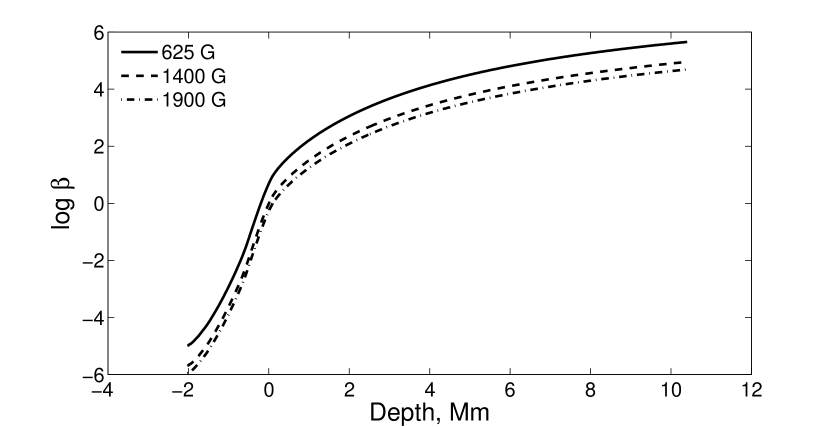
Figure 2: The ratio of the gas pressure to the magnetic pressure (plasma parameter $\beta$) as a function of depth for the background model for three values of the magnetic field strength.

In this section we present our results of numerical simulation of excitation and propagation of MHD waves generated by a single source of vertical force with central frequency $\nu$ = 3.5 mHz placed at depth $h_{src}=100$ km in a rectangular region of size 15.5$\times$15.5$\times$12.5 Mm³ (104$\times$104$\times$70 nodes). The horizontal grid is uniform with $\Delta x=\Delta y=150$ km. The vertical grid is non-uniform. The grid step $\Delta z$ varies from 50 km near the photosphere to 600 km near the bottom of the computational domain. Time step $\Delta t=0.5$ s was chosen to satisfy the Courant stability condition. Vector $\mbox{\boldmath$B$}_{0}=(B_{0}\sin\gamma,0,B_{0}\cos\gamma)^{T}$ of the uniform inclined background magnetic field lies in XZ plane and has inclination angle of $\gamma$ = 45^∘ with respect to the top boundary normal. The magnetic field strength, $B_{0}$, varied from 0 to 2500 G in our simulations. The ratio of the gas pressure to the magnetic pressure, plasma parameter $\beta$ for typical sunspot penumbra values is shown in Fig. 2.

We describe here two examples of wave propagation in the uniform background magnetic field with a wave source located inside the magnetic region, and of a non-uniform magnetic field with the source located outside the magnetic regions. Since the convective motions on the Sun are inhibited in strong magnetic field regions, the acoustic sources there are suppressed. Thus, the second case better describes the realistic situation on the Sun.

The simulation results for the uniform inclined magnetic field of $B_{0}=625$ G are shown in Fig. 3. The vertical map of $B_{z}^{\prime}$ (panel c, right) reveals a strong Alfven wave, which propagates along the background inclined magnetic field lines. As expected, the Alfven wave is not presented in the map of density perturbations. The Alfven wave is generated due to the interaction between the wave source and the magnetic field at the source location. The concentric waves in the left panels represent a mixture of the fast MHD wave (analogous to p-modes in absence of the magnetic field) and the surface magnetic-gravity wave (analogous to f-mode). Since the wave speed depends on the angle between the vectors of magnetic field vector and wavenumber, the wave fronts are anisotropic. The separation of these two types of waves will be discussed in Sec. 3.2 together with analysis of phase and group travel times.

The simulation results for the second case, when the source is placed outside the region containing the background magnetic field are shown in Figure 4. The domain size and grid parameters are the same, as in Figure 3. The background magnetic field $\mbox{\boldmath$B$}_{0}=(0,B_{0}\sin\gamma,B_{0}\cos\gamma)^{T}$ lies in YZ plane, has inclination angle $\gamma$ = 45^∘ with the top boundary normal and is parallel to the planes showed in left columns of figure by dashed lines. The magnetic field $B_{0}$ has constant values of 0 and 2500 G in the regions on the left and right of the dashed lines respectively. Between the dashed lines the strength of the background magnetic field is linearly decreases from maximum value to zero. Such configuration of the background field satisfies condition $\mbox{div}\mbox{\boldmath$B$}_{0}=0$. The magnetic field strength in this example is chosen higher than the typical penumbra value for a better demonstration of the magnetic effects. The wave source is placed in the region free from the background magnetic field. The waves generated by such a source are pure acoustic and surface gravity waves. When they enter the region occupied by the inclined magnetic field they are transformed into the fast MHD and slow magneto-gravity waves respectively. The Alfven wave does not appear in these simulations. Evidently, the fast MHD wave travels faster than the original acoustic wave, and its amplitude is reduced. In these simulations we do not notice significant wave transformation effects in the near surface reflection layers where the plasma parameter, $\beta$, equal to 1. The helioseismic waves are trapped below the surface and according to our simulations are not affected by transformation into other types (slow MHD and Alfven modes). We will discuss in more detail the role of the transformation for waves of different frequencies in a future publication. The main purpose of this paper is to discuss the effects of the inclined magnetic field on the observed travel time variations in the sunspot penumbra.

3.2 Phase and group travel time variations along the wavefront

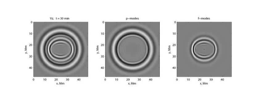
Figure 5: Spectra ($k$–$\nu$ diagrams) and corresponding maps of perturbation of the z-component of velocity are shown on top and bottom rows respectively. Results for the original MHD wave field and wave fields after filtering out $f$- and $p$-modes are shown on panels a, b, and c respectively.

To study the travel time variations we performed simulations in a rectangular box of size 48$\times$48$\times$12.5 Mm³ (320$\times$320$\times$70 nodes) for different values $B_{0}$ and inclination angles $\gamma$ of the uniform background magnetic field: (625 G, 70^∘), (1400 G, 45^∘), and (1900 G, 30^∘). The grid step size, source type and depth were chosen the same as in previous Section 3.1. Total simulation time equals 6 hours of solar time. The simulation results for $B_{0}$=625 G and $\gamma$=70^∘ are shown in Figure 5. The top row represents $k$–$\nu$ diagrams, the bottom one shows corresponded horizontal snapshots of the z-component of velocity at the level of the photosphere for the moment of time $t=30$ min. The usual technique of fitting of the cross-covariance function by Gabor’s wavelet was used to calculate the travel times. This technique was developed for $p$-modes (Kosovichev & Duvall, 1997). The source of the vertical (z-component) of force generates a strong gravity wave (the lowest ridge of $k$–$\nu$ diagram on panel a corresponds to the $f$-mode) which has to be filtered out. Results of separation of $p$- and $f$-modes are shown in panels (b) and (c) respectively. The maps of $V_{z}$ for $p$- and $f$-modes (bottom row) were obtained by taking the inverse Fourier transform of the corresponding 3D spectra. It is clear, even without applying an $f$-mode filter, that starting form the distance of about 15 Mm from the source the $p$- and $f$-modes are spatially separated due to the different velocities. Due to the different dispersion relations the magnetic-gravity and fast MHD waves easily separated on time-distance diagram (see Figure 6). The solid black curve represents a theoretical time-distance curve for $p$-modes and standard solar model in absence of the magnetic field. We see, that the fast MHD waves are not significantly affected by the magnetic field and follow the theoretical $p$-mode curve, calculated for the quiet Sun in the ray approximation (Kosovichev & Duvall, 1997). The magnetic-gravity waves have characteristic ”zebra” structure due to the difference between phase and group velocities. Their speed is less than the speed of the fast MHD wave.

The magnetic field results in anisotropy of the wave properties. Therefore, the wave travel times measured from the line-of-sight component of the displacement velocity depend on the direction of the wave propagation and also on the viewing angle. We have investigate this effect for the case of the uniform inclined magnetic field. The choice of the coordinate system and geometry are shown in Figure 7. Horizontal XY-plane coincides with the photosphere. The origin of the Cartesian coordinate system is placed at the point O above the wave source (the source itself is at the depth of 100 km below the photosphere). The uniform inclined background magnetic filed lies in the XZ-plane ($B_{y}=0$) and has angle $\gamma=45^{\circ}$ with the normal to the photosphere. The location of point of observations $P_{\mathrm{obs}}$ is defined by the distance $\Delta$ from the wave source and the azimuthal angle $\alpha$. The line-of-sight (LoS) direction is defined by two angles: angle $\theta$ between LoS direction and local normal, and azimuthal angle $\psi$ between OX axis and projection of the LoS on the local horizontal plane. First, we build 3D $k$–$\nu$ diagrams for each velocity component $u$, $v$, and $w$, filter out the $f$-modes as shown in Figure 5 and calculate the Cartesian components of velocity perturbation $u_{p}$, $v_{p}$, and $w_{p}$ for $p$-modes by taking the inverse Fourier transform of corresponding spectra. Then, we calculate cross covariance

$$C(\mbox{\boldmath$r$}_{1},\mbox{\boldmath$r$}_{2},\tau)=\frac{1}{T}\int_{0}^{T}v_{LoS}^{(p)}(\mbox{\boldmath$r$}_{1},t)v_{LoS}^{(p)}(\mbox{\boldmath$r$}_{2},t+\tau)dt$$ (11)

of LoS velocities

$$v_{LoS}^{(p)}=u_{p}\cos\psi\sin\theta+v_{p}\sin\psi\sin\theta+w_{p}\cos\theta$$ (12)

in the origin of the system of coordinates and in the observational point $P_{\mathrm{obs}}$ ($\Delta=7.9$ Mm). Then we fit the cross covariance function with Gabor’s wavelet

$$G(\Delta,\tau)=A\cos[\omega_{0}(\tau-\tau_{p})]\exp\left[-\frac{\delta\omega^{2}}{4}(\tau-\tau_{g})^{2}\right],$$ (13)

where $\Delta=|\mbox{\boldmath$r$}_{1}-\mbox{\boldmath$r$}_{2}|$ is the distance between points where LoS velocities $v_{LoS}^{(p)}(\mbox{\boldmath$r$}_{1},t)$ and $v_{LoS}^{(p)}(\mbox{\boldmath$r$}_{2},t)$ are measured, $A$ is the amplitude, $\omega_{0}$ is the central frequency, $\tau_{p}$ and $\tau_{g}$ are the phase and group travel times respectively, and $\delta\omega$ is the bandwidth. Parameters $A$, $\omega_{0}$, $\tau_{p}$, $\tau_{g}$, and $\delta\omega$ are free and have to be determined from the fitting procedure. Repeating this procedure for different observational points with the same $\Delta$ but different azimuthal angle we obtain $\tau_{p}$ and $\tau_{g}$ as functions of $\alpha$.

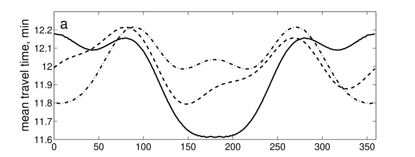
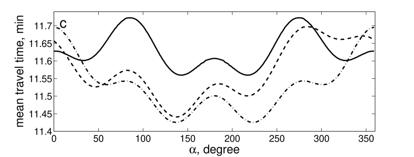
Figure 8: Mean phase travel times vs. azimuthal angle $\alpha$ calculated from Doppler LoS velocities at the hight of 300 km above the photosphere for different strengths of the uniform inclined background magnetic field (625 G for panel a, 1400 G for panel b, and 1900 G for panel c), and different LoS directions. Solid, dashed, and dash-dotted curves represent travel time variations for $\psi$ = $0^{\circ}$, $90^{\circ}$, and $180^{\circ}$ respectively.

Travel time variations along the wave front for different $B_{0}$ and different LoS angles are shown in Figure 8. Panels a, b, and c correspond to $B_{0}$ of 625 G, 1400 G, and 1900 G respectively. The solid, dashed, and dash-dotted curves correspond to $\psi$ = {0^∘, 90^∘, 180^∘} respectively. The angle between the LoS and the local normal is $\theta=20.5^{\circ}$. The mean phase travel times show variations of about 0.5 min along the wave front, the variation amplitude is a little smaller for strong (1400–1900 G) magnetic fields than for the weak 625 G field. For the weak magnetic field changes of $\psi$ change the shape of the curve, but not its average value. The strong magnetic fields cause anisotropy, and the mean value of the travel times changes with angle $\psi$. Thus, averaging along the wave front for the strong magnetic fields gives variations of the observed mean travel times of about 0.1–0.3 min with angle $\psi$ (see detailed discussion in the next section).

3.3 Azimuthal dependence of phase travel times in sunspots: comparison with observations

Zhao & Kosovichev (2006) observed different behavior of azimuthal dependence of phase travel times obtained from the SOHO/MDI Doppler shift data (Scherrer et al., 1995) in sunspots depending on their position on the disk. As far as we want to reproduce similar conditions (and geometry) in our simulations we give a detailed description of their algorithm of the phase travel time calculation. We will apply the same technique to our simulated data.

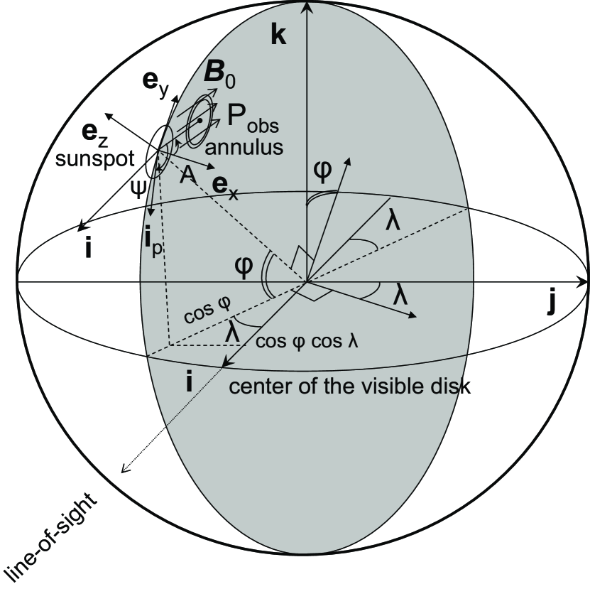
Figure 9: To derivation of the relation between $\psi$ and $A$. Angle $A$ is the azimuthal angle of the observation point in the local coordinate system associated with the sunspot. Angle $\psi$ is one of two angles determining the LoS direction.

The sunspot is located at latitude $\phi$ and longitude $\lambda$ on the eastern part of the disk as shown in Figure 9. The sunspot meridian plane is shown by gray color. Orth $i$ of the global system of coordinate with the origin in the center of the Sun is aimed at the center of the visible solar disk, orth $k$ points to the north, and orth $j$ points to the west. The local system of coordinates with the origin in the center of the sunspot is chosen in such a way that $\mbox{\boldmath$e$}_{z}$ coincides with the local normal to the surface, $\mbox{\boldmath$e$}_{x}$ is directed to the west, and $\mbox{\boldmath$e$}_{y}$ is directed along the meridian and forms a right vector triplet with $\mbox{\boldmath$e$}_{z}$ and $\mbox{\boldmath$e$}_{y}$.

Observational point $P_{\mathrm{obs}}$ is chosen inside the sunspot penumbra. Azimuthal angle $A$ is counted counterclockwise from local west direction $\mbox{\boldmath$e$}_{x}$. Two signals are calculated: the LoS velocity at $P_{\mathrm{obs}}$ and the LoS velocity averaged along the annulus (between inner and outer radii of a ring with average radius $\Delta$ = 8 Mm with the origin in the observational point). Cross covariance of these two signals is fit with the Gabor s wavelet. Fitting procedure gives us mean phase and group travel times. We assume, that the annulus is small enough that sunspot magnetic field $\mbox{\boldmath$B$}_{0}$ inside the annulus can be considered as uniform. Hence the problem is reduced to simulations with the uniform inclined magnetic field shown in Figure 5. To compare results of the simulations with the observations we have to find from what direction we have to look at our simulation domain to match the observations. In other words, we have to find a relation between azimuthal angle $A$ of the sunspot center and $\psi$. Angle $\psi$ here has the same meaning as in Figure 7. This is the angle between the projection of the background magnetic field on the local horizon (XY-plane) and projection of the LoS on the same plane. The unit vector in LoS direction in the sunspot local system of coordinates is given by equation

$$\mbox{\boldmath$i$}=\sin\lambda\;\mbox{\boldmath$e$}_{x}-\sin\phi\cos\lambda\;\mbox{\boldmath$e$}_{y}+\cos\phi\cos\lambda\;\mbox{\boldmath$e$}_{z}.$$ (14)

The projection of $i$ on local horizontal plane (defined by vectors $\mbox{\boldmath$e$}_{x}$ and $\mbox{\boldmath$e$}_{y}$) has coordinates $\mbox{\boldmath$i$}_{p}=(-\sin\lambda,-\sin\phi\cos\lambda,0)^{T}$ (non-unit vector). Angle $\psi$ is given by equation

$$\psi=-A-\angle\mbox{\boldmath$i$}_{p}\mbox{\boldmath$e$}_{x}=-A-\arccos\left(\frac{-\sin\lambda}{\sqrt{\sin^{2}\lambda+\sin^{2}\phi\cos^{2}\lambda}}\right).$$ (15)

We performed numerical simulations of propagation of MHD waves in presence of the uniform inclined magnetic field for different inclination angles and strengths of the magnetic field. The goal of these simulations was to calculate contribution of the inclined magnetic field effect to variations of the mean travel times with the azimuthal angle. This is why we used horizontally uniform standard solar model as a background model. The same model was used to obtain Figures 3, 4. The mean travel times obtained for the photospheric level (panel a) and the level of 300 km above the photosphere (panel b) are shown in Figure 10. The solid curve corresponds to the magnetic field $B_{0}=625$ G with inclination angle $\gamma=70^{\circ}$. The dashed and dash-dotted curves are corresponded to cases $B_{0}=1400$ G, $\gamma=45^{\circ}$ and $B_{0}=1900$ G, $\gamma=30^{\circ}$ respectively. The systematic shift of the calculated mean travel times with respect to the observations is caused by temperature effects (the sound speed is smaller inside sunspots than in the quiet Sun), which are not included in these simulations. The travel times systematically decrease when the strength of the magnetic field increases because the speed of the fast MHD wave increases with the magnetic field. For studying the inclined field effect we are mostly interested in relative variations of the mean travel times, provide the absolute values to give a general impression about the magnitude of contributions to the mean travel times from the temperature effect and variations of the fast MHD wave speed with the magnetic field. A model of a sunspot with both temperature and magnetic field effect will be presented in a future publication.

The amplitude of the mean travel time variations for weak (625 G) magnetic field is 10 times smaller than the observed quantity for the height of 300 km and even smaller for the photospheric level. For stronger magnetic fields (1400–1900 G) the amplitude of travel time variations is about 25% of the observed amplitude. Behavior of the travel times depends on the magnetic field strength and the level of observation of Doppler velocities. For the weak magnetic field (625 G) the phase of the travel time variations is opposite to the observations for both levels. For the height of 300 km above the photosphere where plasma parameter $\beta\ll 1$ simulated travel times show the same phase as in observations for both magnetic field strengths (1400 G and 1900 G). For the photospheric level and field strength of 1900 G the phase of travel time variations coincides with the observations, while the travel time variations for $B_{0}=1400$ G are in antiphase with the observations. Comparison of the curves at different heights for the same inclination angles and magnetic field strengths shows that for the photospheric layer the mean travel times are systematically smaller by only about 0.12 min than for the layer of 300 km above the photosphere. Thus, the variations in the height of Doppler shift measurement do not have a significant effect.

The curves in Figure 10 were obtained for the annulus radius of 8 Mm and the sunspot located at heliospheric latitude $\phi=19.5^{\circ}$ and longitude $\lambda=-6.5^{\circ}$. The angle between LoS and local normal to the photosphere at the center of the sunspot ($\theta$ angle) is $20.5^{\circ}$. The parameters are chosen to match corresponded angles for Figure 1b of Zhao & Kosovichev (2006).

4 Conclusion

The numerical 3D simulations of excitation and propagation of magneto-acoustic-gravity waves in the solar interior and atmosphere show that the presence of the inclined background magnetic field significantly alters properties of $f$-modes but has little effect on $p$-modes. The interaction of the wave source with the background magnetic field generates a strong Alfven wave. However, the Alfven wave does not appear when the wave source is located outside the magnetic region, and the acoustic-gravity waves propagate from the region without magnetic field into the region with magnetic field.

The helioseismic travel times, obtained from cross covariance of the $p$-mode LoS velocities at the observation point and the source point, show variations of about 1 min along the wave front (the amplitude depends on inclination $\theta$ of the LoS). Due to the anisotropy, the travel time averaged along the wave front (like in the observational procedure) is not zero. Comparison of the variations of the mean travel times vs. the azimuthal angle of the observing point shows that the simulation results are in phase with the observations when Doppler velocities are taken at the level of 300 km above the photosphere (at the same height as the observed velocities are obtained). The travel time weakly depends on the height of observations. The amplitude of variations of the travel times obtained form simulations is about 25% of the observed amplitude even for strong fields of 1400–1990 G. It can be an indication that other effects (for example background flows or non-uniform distribution of magnetic field) can contribute to the observed travel time variations. The developed 3D MHD wave propagation code provides an important tool for further investigations of local helioseismology in regions with the strong magnetic field.

5 Acknowledgements

We thank to Junwei Zhao for providing us data of variation of the mean travel times obtained from observations of sunspots. Calculations were carried out on Columbia supercomputer of NASA Ames Research Center.

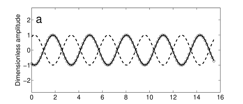
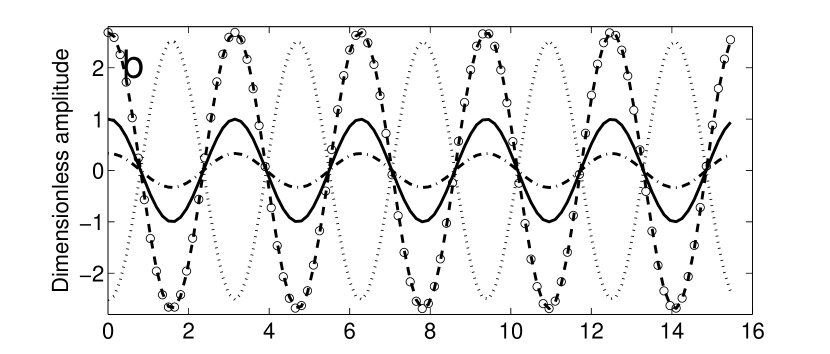
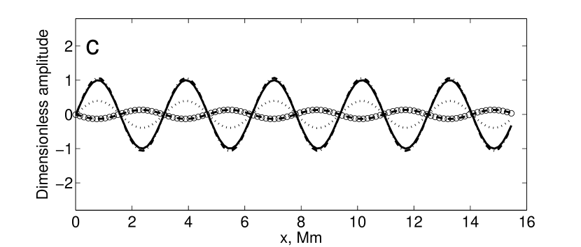
Figure 1: Comparison of analytic (cirves) and numerical (markers) solutions for plain Alfven (a), slow MHD (b), and fast MHD (c) waves respectively. For Alfven wave only $v$ and $B_{y}$ (marked by solid and dashed curves respectively) are non-zero. Circles mark an analytical solution for $v$. Solid, dash-dotted, dashed, and dotted curves in panels (b) and (c) correspond to $\rho$, $u$, $w$, and $B_{z}$ respectively. Analytical solution for $w$ is shown by circles.

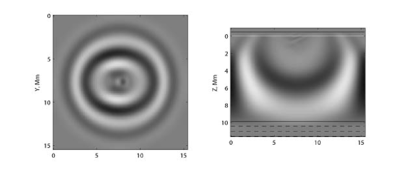
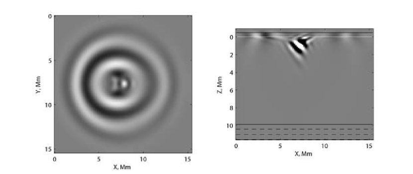
Figure 3: Snapshots of horizontal (left column) and vertical (right column) slices of the 3D domain for perturbations of density $\rho$ (a), z-momentum $\rho_{0}w$ (b), and z-component of the magnetic field $B_{z}$ (c). Strong Alfven wave is generated due to the interaction of the wave source and the background magnetic field at the source location. In this example, $B_{0}=625$ G, and inclined by $45^{\circ}$ in the XY-plane.

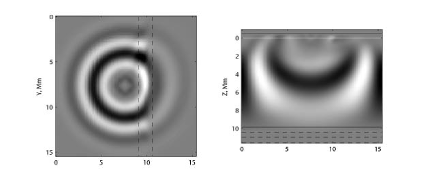
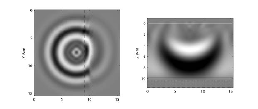
Figure 4: Snapshots of horizontal (left column) and vertical (right column) slices of the 3D domain for perturbations of density $\rho$ (a), z-momentum $\rho_{0}w$ (b), and z-component of the magnetic field $B_{z}$ (c). The strength of the background magnetic field (inclined by $45^{\circ}$ in the YZ-plane) is 2500 G in the region to the right from vertical dashed lines in left column and 0 in the left region. The wave source is located in the region free of magnetic field. Propagating into the region with the background magnetic field acoustic and surface gravity waves are transformed into the fast MHD wave and magneto-gravity wave. The Alfven wave does not appear in this case.

Figure 6: Time-distance diagram for density perturbations. Solid curve represents a theoretical time-distance curve for $p$-modes and the standard solar model in absence of the magnetic field. Fast MHD wave and magnetic-gravity waves are separated due to the different dispersion relations.

Figure 7: Choice of the coordinate system. The line-of-sight direction is defined by angles $\psi$ and $\theta$. Position of observational point $P_{\mathrm{obs}}$ on the photosphere is fixed by azimuthal angle $\alpha$ and distance $\Delta$ from the projection of wave source O.

Figure 10: Phase travel time obtained from simulations averaged along with annulus with radius 8 Mm as a function of azimuthal angle $A$. The solid, dashed, and dot-dashed curves corresponds to the following combinations of the magnetic field strength and inclination angles: (i) $B_{0}=625$ G, $\gamma=70^{\circ}$, (ii) $B_{0}=1400$ G, $\gamma=45^{\circ}$, (iii) $B_{0}=1900$ G, $\gamma=30^{\circ}$. Data points with errorbars represent observations.

References

- Bogdan (2000) Bogdan T.J. 2000, Sol. Phys., 129, 373
- Christensen-Dalsgaard et al. (1996) Christensen-Dalsgaard, J., et al. 1996, Science, 272, 1286
- Duvall et al. (1996) Duvall, T. L. J., D’Silva, S., Jefferies, S. M., Harvey, J. W., & Schou, J. 1996, Nature, 379, 235
- Georgobiani et al. (2007) Georgobiani, D., Zhao, J., Kosovichev, A. G., Benson, D., Stein, R. F., & Nordlund, Å. 2007, ApJ, 657, 1157
- Haber et al. (2000) Haber, D. A., Hindman, B. W., Toomre, J., Bogart, R. S., Thompson, M. J., & Hill, F. 2000, Sol. Phys., 192, 335
- Komm et al. (2008) Komm, R., Morita, S., Howe, R., & Hill, F. 2008, ApJ, 672, 1254
- Kosovichev (1996) Kosovichev, A. G. 1996, ApJ, 461, L55
- Kosovichev & Duvall (1997) Kosovichev, A. G., & Duvall, T. L., Jr. 1997, SCORe’96 : Solar Convection and Oscillations and their Relationship, 225, 241
- Kosovichev et al. (2000) Kosovichev, A. G., Duvall, T. L. _. J., & Scherrer, P. H. 2000, Sol. Phys., 192, 159
- Nigam et al. (2007) Nigam, R., Kosovichev, A. G., & Scherrer, P. H. 2007, ApJ, 659, 1736
- Parchevsky & Kosovichev (2007a) Parchevsky, K. V. and Kosovichev, A. G. 2007a, ApJ, 666, 547
- Parchevsky & Kosovichev (2007b) Parchevsky, K. V., & Kosovichev, A. G. 2007b, ApJ, 666, L53
- Parchevsky et al. (2008) Parchevsky, K. V., Zhao, J., & Kosovichev, A. G. 2008, ArXiv e-prints, 802, arXiv:0802.3866
- Rajaguru et al. (2006) Rajaguru, S. P., Birch, A. C., Duvall, T. L., Jr., Thompson, M. J., & Zhao, J. 2006, ApJ, 646, 543
- Scherrer et al. (1995) Scherrer, P. H., et al. 1995, Sol. Phys., 162, 129
- Schunker et al. (2005) Schunker, H., Braun, D. C., Cally, P. S., & Lindsey, C. 2005, ApJ, 621, L149
- Vernazza et al. (1976) Vernazza, J. E., Avrett, E. H., and Loeser, R. 1976, ApJS, 30, 1.
- Unno et al. (1989) Unno, W., Osaki, Y., Ando, H., Saio, H., & Shibahashi, H. 1989, Nonradial oscillations of stars, Tokyo: University of Tokyo Press, 1989, 2nd ed.,
- Zhao et al. (2001) Zhao, J., Kosovichev, A. G., & Duvall, T. L., Jr. 2001, ApJ, 557, 384
- Zhao & Kosovichev (2006) Zhao, J. and Kosovichev, A.,G. 2006, ApJ, 643, 1317.
- Zhao et al. (2007) Zhao, J., Georgobiani, D., Kosovichev, A. G., Benson, D., Stein, R. F., & Nordlund, Å. 2007, ApJ, 659, 848