The X-ray Halo of Cen X-3

Abstract

Using two Chandra observations we have derived estimates of the dust distribution and distance to the eclipsing high mass X-ray binary (HMXB) Cen X-3 using the energy-resolved dust-scattered X-ray halo. By comparing the observed X-ray halos in 200 eV bands from 2–5 keV to the halo profiles predicted by the Weingartner & Draine interstellar grain model, we find that the vast majority ($\approx$70%) of the dust along the line of sight to the system is located within about 300 pc of the Sun, although the halo measurements are insensitive to dust very close to the source. One of the Chandra observations occurred during an egress from eclipse as the pulsar emerged from behind the mass-donating primary. By comparing model halo light curves during this transition to the halo measurements, a source distance of $5.7\pm 1.5$ kpc (68% confidence level) is estimated, although we find this result depends on the distribution of dust on very small scales. Nevertheless, this value is marginally inconsistent with the commonly accepted distance to Cen X-3 of 8 kpc. We also find that the energy scaling of the scattering optical depth predicted by the Weingartner & Draine interstellar grain model does not accurately represent the results determined by X-ray halo studies of Cen X-3. Relative to the model, there appears to be less scattering at low energies or more scattering at high energies in Cen X-3.

1. Introduction

X-ray halos, which appear as diffuse emission surrounding X-ray sources, are created by small-angle scattering of soft X-ray photons from dust grains in the interstellar medium (ISM). Their study can provide information on interstellar grain properties (density, morphology, composition) and on the spatial distribution along the line of sight. Given a dust distribution, variability in the X-ray halo can be used to geometrically derive estimates of the distances to X-ray sources based on the time delays of the photons scattered along the line of sight (Trümper & Schönfelder, 1973). This method has been applied in a number of cases (e.g., Predehl et al., 2000; Thompson et al., 2006; Audley et al., 2006; Xiang et al., 2007). The goal of this work is to estimate the dust distribution and distance to the eclipsing HMXB Cen X-3 using measurements of its dust-scattered halo with the Chandra X-Ray Observatory.

The theory of X-ray scattering and the production of X-ray halos has been described by a number of authors (e.g., Mathis & Lee 1991, Smith & Dwek 1998, Draine 2003). Various interstellar grain models have been proposed. Mathis et al. (1977) developed a model composed of silicate and graphite grains with a size distribution of $n(a)\propto a^{-3.5}$, which reproduces the observed extinction of starlight. Weingartner & Drain (2001, hereafter WD01) produced a grain model that additionally accounts for the diffuse infrared and microwave emission emission from the ISM by including sufficient small carbonaceous grains and polycyclic aromatic hydrocarbons (PAHs). Zubko et al. (2004) created a series of models by simultaneously fitting the extinction, infrared emission, and elemental abundance constraints, by including, for example, amorphous carbon particles, organic refractory material, water ice, and voids.

One of the many challenges in developing a viable model is that the characteristics of the dust may vary in different Galactic locations due to different local evolutionary histories, ISM phases, and abundances of elements. Given such difficulties, a preeminent interstellar grain model has not been established. For our purposes, we use the WD01 grain model, although we allow the energy dependence of the scattering cross section to be a free parameter.

The basic quantity that determines the characteristics of X-ray halos is the differential scattering cross section $d\sigma/d\Omega$. This can be calculated using the exact Mie solution or the simpler Rayleigh-Gans approximation. For the WD01 grain model, the differential scattering cross section as a function of scattering angle $\phi$ can be approximated by the simple analytic form

$$\frac{d\sigma}{d\Omega}\approx\frac{\sigma_{\rm sca}}{\pi\phi^{2}_{{\rm s},50}}\left[1+\left(\frac{\phi}{\phi_{{\rm s},50}}\right)^{2}\right]^{-2}$$ (1)

where $\phi_{{\rm s},50}\approx 360\arcsec~{}({\rm keV}/E)$ is the median scattering angle as a function energy (Draine 2003). It is important to note that the following results are probably somewhat dependent on this chosen form of the differential scattering cross section.

Cen X-3 is one of the brightest accreting X-ray pulsars, and it is one of the six pulsars in which the observation of eclipses has permitted the determination of all orbital and stellar parameters. The rotation period of the pulsar is 4.8 s, and the binary orbital period is 2.1 days. The inclination of the orbital plane and the mass of the neutron star have been estimated to be $i\sim 70^{\circ}$ and $M=1.21\pm 0.21$ ${M}_{\mathord{\odot}}$ (Ash et al. 1999). The optical counterpart of Cen X-3 has been identified as an early type star of radius $R\sim 12$ ${R}_{\mathord{\odot}}$ and mass $M\sim 20$ ${M}_{\mathord{\odot}}$ (Rappaport & Joss, 1983). Accretion in the system probably occurs via an accretion disk (Bildsten 1997; Takeshima et al. 1992), although the mass transfer mechanism probably includes an X-ray excited wind (Day & Stevens, 1993).

Although well-studied, the distance to Cen X-3 remains uncertain. Using a B0 II stellar classification model, an 8 kpc distance to Cen X-3 was obtained (Krzemiński, 1974), however, subsequent work indicated that the supergiant primary was of type O6–-8 III (Hutchings et al. 1979). Day & Tennant (1991) observed soft emission during two eclipses using EXOSAT and attributed it to the dust-scattered halo, from which they derived a distance of $5.4\pm 0.3$ kpc. Discrepancies of $\sim$2.5 kpc in distance estimates to Cen X-3 lead to nearly a factor of two difference in the inferred optical and X-ray luminosities.

Cen X-3 ($l=292\fdg 09,b=0\fdg 34$) is particularly suited for X-ray halo studies. The source is usually very bright, and the interstellar hydrogen column density along the line of sight is $1.20\times 10^{22}$ cm^-2 (Dickey & Lockman, 1990), implying a large enough optical depth to result in an appreciable halo (Predehl & Schmitt, 1995), yet not so large as to include a substantial contribution due to multiply scattered photons. Moreover, the eclipsing nature of the binary system is advantageous because it should produce the largest fraction of variability in the X-ray halo, which makes a geometric distance measurement more direct.

Section 2 presents the general equations that characterize the shape and variability of X-ray halos. For our study of the X-ray halo of Cen X-3, two Chandra High Energy Transmission Grating (HETG) observations are used; one observation took place outside of eclipse ($\Phi_{\rm orb}\sim 0.4-0.6$) when there was little variability in the flux (hereafter, called the “plateau” phase of the orbit based on the shape of the light curve), and the other occurred during an egress from eclipse (§ 3). Because accurate halo measurements critically depend on careful subtraction of the instrumental point spread function (PSF), the shape and normalization of the PSF is parametrized using all Chandra/HETG observations of the unabsorbed sources Her X-1 and PKS 2155-304. These results are presented in the appendix to the paper. The method for deriving the dust distribution to Cen X-3 is discussed in § 4.1. With a dust distribution established, the large amplitude change in flux during eclipse egress is used to constrain the distance to the system (§ 4.2). A comparison of the inferred dust distribution to observations of CO emission, star counts, and interstellar extinction in the direction of Cen X-3 is presented in § 4.3. We discuss the implications of our results in § 5, and we provide a brief summary in § 6.

2. X-ray Halos

Following Draine & Tan (2003; hereafter DT03), for a steady source, the intensity of single-scattered photons arriving at halo angle $\theta$ is given by

$$I_{1}(\theta)=F_{\rm X}\tau_{\rm sca}\tilde{I}_{1}(\theta),$$ (2)

where $F_{\rm X}$ and $\tau_{\rm sca}$ are the flux and scattering optical depth, respectively, where

$$\tilde{I}_{1}(\theta)\approx\int_{0}^{1}\frac{\tilde{\rho}(x)}{(1-x)^{2}}\frac{d\sigma}{d\Omega}dx,$$ (3)

$\tilde{\rho}(x)$ is the dimensionless dust density at fractional distance $x$ to the source, the scattering angle and the halo angle are related through $\phi\approx\theta/(1-x)$, and the normalization is chosen such that $\int\tilde{I}_{1}(\theta)2\pi\theta d\theta=1$. For a variable source, a photon appearing at halo angle $\theta$ after scattering from a dust grain at a fractional distance $x$ to a source $D$ kpc away will be delayed with respect to the central source by

$$\delta t=1.21\frac{D}{\rm kpc}\left(\frac{\theta}{\rm arcsec}\right)^{2}\frac{x}{1-x}~{}{\rm s}.$$ (4)

In this case, $F_{\rm X}$ must be moved inside the integral (eq. 3) because the halo flux at time $t$ is proportional the flux of the central point source at the “retarded time” $t^{\prime}=t-\delta t$, i.e., $I_{1}(t,\theta)\propto F_{\rm X}(t-\delta t(x,\theta))$.

It is clear that to accurately determine the proportionality between the source flux and the halo, one must know the history of the source flux for a sufficiently long time period preceding the observation. In most cases this is not practical, so typically one assumes that any change in the source flux took place sufficiently long ago for the halo to have completely responded to it (as we do when estimating the dust distribution, § 4.1), or one models the history of the source flux using reasonable estimates (as we do when constraining the source distance, § 4.2).

The intensity of the X-ray halo due to photons scattering two or more times ($I_{2}$, $I_{3}$, …) is straightforward for a steady source given an assumed dust distribution, and we refer the reader to DT03 for the appropriate recursion formula. However, accounting for the time delays for multiply-scattered photons is extremely cumbersome. Fortunately, the intensity of the halo due to photons scattered $n$-times, relative to the observed source flux, is $\tau_{\rm sca}^{n}/n!$ (Mathis & Lee, 1991), so the halo intensity for multiply-scattered photons decreases rapidly for reasonably small optical depths ($\tau_{\rm sca}\lesssim 2$). Usually, the first- and second-order scatterings are sufficient to model the total halo.

3. Observations & Data Extraction

In this paper, we use two Chandra/HETG observations of Cen X-3 (ObsIDs 1943 & 7511), and several Chandra/HETG observations of PKS 2155-304 and Her X-1 to model the PSF (see the appendix). Although the use of the grating reduces the zeroth-order image count rate by about a factor of 3, the dispersed spectrum provides accurate measurements of the source flux and spectrum, which is necessary to accurately model the characteristics of the X-ray halo and the PSF. One of the observations (ObsID 1943) began at MJD 51908.01 and lasted for 45 ks, corresponding to $\Phi_{\rm orb}\approx 0.38-0.63$, where determination of the orbital phases was accomplished using the mid-eclipse ephemeris from Burderi et al. (2000), and the orbital period and evolution $[\mbox{\.{\em P}}_{\rm orb}/P_{\rm orb}=-(1.738\pm 0.004)\times 10^{-6}$ yr${}^{-1}]$ from Nagase et al. (1992). A dip in the flux was observed at about $\Phi_{\rm orb}\approx 0.57$, so we ignored data after this time to simplify analysis by removing any time dependence (eq. 4). X-ray halo measurements from this observation were used to estimate the dust distribution along the line of sight. The other observation of Cen X-3 (ObsID 7511), which resulted from a successful observing proposal with the primary goal of geometrically estimating the distance to the system, took place during an egress from eclipse. The 40 ks observation began at MJD 54355.46 ($\Phi_{\rm orb}\approx 0.08-0.30$). The preceding mid-eclipse epoch was calculated to be MJD $54355.313\pm 0.007$. Figure 1 (top-left panel, solid curve) shows the Chandra/HETG light curve during the eclipse egress observation. We also present an RXTE/PCA light curve for comparison. Clearly, the Chandra observation occurred during a relatively lower flux state, leading to a more gradual increase in flux coming out of eclipse as compared the PCA observation. Priedhorsky & Terrell (1983) discussed the aperiodic 120–165 day timescale between the different flux states, and Clark et al. (1988) studied how the stellar wind and the shape of the egress light curves are affected by the different states.

Figure 1.— Comparison of the eclipses and flux states in count rates (left panels) and fluxes (right panel) from 3–5 keV between the Chandra eclipse egress observation (ObsID 7511) and an RXTE/PCA observation. No data were obtained for the Chandra eclipse ingress (dotted curve). The ingress is modelled as the mirror image of the egress (multiplied by 0.87, see § 4.2).

Data analysis was performed using the standard tools of the Chandra Interactive Analysis of Observations (CIAO) software version 4.0 and Calibration Database (CALDB) version 3.4.3. A single first-order Medium Energy Grating (MEG) and High Energy Grating (HEG) spectrum was extracted for the plateau phase observation (ObsID 1943). For the eclipse egress observation (ObsID 7511), ten 3968 s first-order MEG/HEG spectra were extracted to model the evolution of the point source spectrum. Spectral models were fit to each spectrum using XSPEC version 11.3, and fluxes (in units of [photons/cm²/s]) were measured in 15 energy bands of 200 eV width from 2–5 keV. Finer time resolution on the flux evolution was obtained by comparing the average HETG count rates in each time range and energy band to the relative count rates in smaller 100 s time bins.

Separate X-ray halo images and exposure maps were extracted in 200 eV bands from 2–5 keV, from which we obtained exposure-corrected surface brightness distributions using 40 logarithmically-spaced annular regions surrounding the source. For the plateau phase observation, a single exposure map was created for each energy band. On the other hand, accurate measurements of the evolution of the halo flux in each energy band during the eclipse egress observation required the use of separate exposure maps (due to the dither of the telescope) using 500 s bins (1200 exposure maps in total). Due to issues with the diffracted HETG photons confusing the background analysis (HETG photons create a diffuse “transfer swath” analogous to the “transfer streak” in the zeroth-order image), we did not use halo angles greater than 110″. The surface brightness distributions were divided by the flux measurements in each band to produce images in units of flux fraction per square arcsecond. Halo angles smaller than about 3″ are affected by pile-up and ignored. To minimize concerns due to multiply-scattered photons, we excluded energies below 2 keV in each observation.

Figure 2.— Cen X-3 halo measurements and best-fit model halos (§ 4.1) shown in three bands from 2–5 keV in units of source flux per square arcsecond. Note that the actual fits to the halos used 200 eV bands. Larger 1 keV bins are displayed to facilitate the visual comparison between the models and the data. The dotted curves show the contribution to the halo from the individual single-scattered ($\Delta x=0.05$) clouds (see Fig. 3 for the cloud locations), the dashed curves show the halo contribution from photons scattered twice, and the solid curves show the sum of the single- and double-scattered halos ($\chi^{2}_{\nu}=1.05$, 502 dof). Third- and higher-order scatterings are nearly negligible and are not included in the model.

In the appendix, we parametrize the PSF as the fraction of the point source flux comprising the PSF as a function of halo angle. Although the observed surface brightness distributions represent the convolution of the PSF and the X-ray halo, in our analysis we treat it as the sum. This is acceptable because we restrict our investigation to angular scales that are much larger than the $\sim$0$\farcs$5 resolution of the telescope mirrors. The PSF contribution in each energy band is simply subtracted from the observed surface brightness distribution. The resulting X-ray halos, rebinned in 1 keV bands, are shown in Figure 2. The fitted halo components are discussed below.

4. Analysis & Results

4.1. Estimating the Dust Distribution

In order to estimate the dust distribution to Cen X-3, we used the plateau phase Chandra observation. We assumed the halo had sufficient time to respond to the eclipse egress, which based on the orbital ephemeris occurred $\sim$30 ks earlier. Once we established a dust distribution, we checked whether or not the assumption was acceptable. First, we created separate single-scattered X-ray halo profiles for twenty step-function dust distributions of width $\Delta x=0.05$ (hereafter referred to as “clouds”), spanning the entire line of sight, i.e., 0.00 to 0.05, 0.05 to 0.10, and so on, for each energy band. By summing the twenty profiles with equal weighting, one could obtain the single-scattered X-ray halo for dust distributed uniformly along the line of sight. The normalization of each cloud ($a_{x}$), which is proportional to the contribution to the total scattering optical depth (due to the normalization $\int\tilde{I}_{1}(\theta)2\pi\theta d\theta=1$), was allowed to vary freely. The initial fit function at each energy is

$$\frac{I_{\rm sca}(\theta)}{F_{\rm X}}=\sum\limits_{x=0}^{19}a_{x}\tilde{I}_{1}^{x}(\theta),$$ (5)

where

$$\tilde{I}_{1}^{x}(\theta)\approx\int_{0.05x}^{0.05(x+1)}\frac{1}{(1-x)^{2}}\frac{d\sigma}{d\Omega}dx.$$ (6)

Note that the superscript in $\tilde{I}_{1}^{x}$ is a label that indicates a position along the line of sight and is not an exponent. Using this method, the dimensionless dust density and scattering optical depth are simply

$$\tilde{\rho}(x)=\frac{a_{x}}{\sum a_{x}},~{}\sum a_{x}=\tau_{\rm sca},$$ (7)

respectively. The halos for each energy band were fit simultaneously. For the initial fit, we used the energy scaling of the scattering optical depth from the WD01 interstellar grain model ($R_{V}=3.1$); however, we found it to underpredict the halo flux at higher energies (or overpredict the flux at lower energies). We therefore allowed the energy scaling to also be a free parameter, although we required that it be a smooth function, i.e., $\tau_{\rm sca}(E)\propto(E-E_{0})^{-\beta}$, where $E_{0}$ and $\beta$ are fit parameters. Nevertheless, the angular dependence of the scattering at a particular energy still follows the functional form predicted by the WD01 model (see eq. [1]). The best-fit normalization of each cloud provided a preliminary dust distribution. Given the preliminary model, the X-ray halo for double-scattered photons was calculated ($I_{2}(\theta)$), included in the model as an additional term in eq. (5), and the normalization for each cloud was refit. This process was repeated in an iterative manner to coverage to the dust distribution whose single- and double-scattered X-ray halos accurately described the Cen X-3 halo. Third- and higher-order scatterings were ignored, but their contribution to the halo is negligible. The Cen X-3 X-ray halos in units of source flux and the best-fit halo models are presented in Figure 2, and the integrated (2–5 keV) surface brightness distribution is shown in Figure 3. Evidently, the 3″–100″ halo can be modeled using only four separate dust clouds (Fig. 3, dotted curves).

The energy dependence of the scattering optical depth is presented in Figure 4, showing the relatively brighter halo at higher energies as compared to the WD01 interstellar grain model predictions (see discussion). The Cyg X-1 and GX 13+1 points are the same data as presented in Fig. 11 of Draine (2003), who compared the optical depth calculated from the WD01 model to observations. Although Draine (2003) extended his comparison to other sources, only Cyg X-1 and GX 13+1 span the 2–5 keV energy range that we investigate for Cen X-3.

Figure 3.— Surface brightness distribution (with PSF subtracted) from 2–5 keV. As in Fig. 2, the dotted curves show the contribution to the halo from the individual ($\Delta x=0.05$) clouds and the dashed curves show the halo contribution from photons scattered twice. The location of the dust for each single-scattered halo component is labelled at left (also see Fig. 5).

Figure 4.— Best-fit scattering optical depth to Cen X-3 as a function of energy (solid curve). The empirical best-fit curve is described by $\tau_{\rm sca}(E)\propto(E-E_{0})^{-\beta}$, where $E_{0}\sim 1.96$ and $\beta\sim 0.32$. The optical depth predicted by the WD01 interstellar grain model ($R_{V}=3.1$) is shown as a dash-dotted curve. The normalization for the WD01 model was chosen so that the areas under each curve are the same. Also included are Cyg X-1 data from Yao et al. (2003) (filled circles) and GX 13+1 data from Smith et al. (2002) (triangles) (see discussion). The normalizations for the Cyg X-1 and GX 13+1 data have been modified to more closely align the points with the empirical curve for Cen X-3. The data points from Yao et al. (2003) have been corrected assuming uniform dust, and the data points from Smith et al. (2002) have been corrected assuming the dust density is proportional to distance. See Draine (2003) for further details on the correction method.

One of the primary goals of this work is to geometrically constrain the distance to Cen X-3, therefore it is important to quantify the uncertainty in the dust distribution because this directly affects the size of the time delays of photons scattered along the line of sight. By fixing the double-scattered halo model to the one corresponding to the best-fit dust distribution, the single-parameter 90% confidence uncertainties in the contribution from each of the twenty clouds was calculated. In each case the lower limit on the cloud size was zero, i.e. no dust, simply because the clouds to either side of the cloud in question could produce a surface brightness distribution with a similar shape. On the other hand, the upper limits to the size of each cloud are well-determined. Figure 5 shows the best-fit dust distribution towards Cen X-3 and the single-parameter upper limits for the size of each cloud. Three examples of different dust distributions that are also consistent with X-ray halo data are presented. The majority of the dust ($\approx$70%) in each case is located at small fractional distances to Cen X-3. Note, however, that we do not have reliable data for halo angles less than about 3″, so we are mostly insensitive to dust that produces centrally-peaked halos, i.e., dust very near the source ($x>0.99$). Therefore, it is more accurate to consider the scattering optical depth in Fig. 4 as a lower limit.

Figure 5.— Best-fit model dust distribution to Cen X-3 (solid histogram). The majority of the dust is located near the Sun ($0.00<x<0.05$), and the other primary dust locations are at $x>0.75$. Although the best-fit distribution accurately models the data ($\chi^{2}_{\nu}=1.05$, 502 dof), the size of any individual dust cloud is not well-constrained (dotted histogram). The three small panels labeled $a$, $b$, and $c$ (corresponding to the upper limits shown in the main panel) show examples of dust distributions that are also consistent with the data at the 90% confidence level.

It could be argued that lack of knowledge of the dust very near the source poses a problem for our distance estimate. This is not the case: For an assumed distance of 8 kpc, the $\sim$0$\farcs$5 angular resolution of the Chandra mirrors corresponds to approximately 4000 AU, which, based on the orbital parameters of the binary system, is more than 4 orders of magnitude larger than the semi-major axis of the orbit. Therefore, the point source flux already includes all of the effects due to scattering in the vicinity of the binary system.

Considering the best-fit dust distribution, it is clear that the assumption that the halo during the plateau phase observation had responded to the preceding eclipse egress is not valid for all halo angles. As pointed out above, an estimate of the time Cen X-3 has been out of eclipse at the beginning of the observation is about 30 ks. The causally-connected regions of $x$ vs. $\theta$ phase space for delay times less than 30 ks are shown in Figure 6 for three source distances, indicating that the assumption is invalid for large $x$ and $\theta$. Fortunately, the vast majority of the dust along the line of sight is located at $x<0.05$ which presents no inconsistency, and the two clouds closest to the source ($0.90<x$) dominate the halo at $\theta\lesssim 10\arcsec$ (see Fig. 3), where the halo angles are small enough to have responded to the previous eclipse egress. The only potential problem concerns the $x=[0.75,0.80]$ dust cloud, which for $\theta\gtrsim 30\arcsec$ have not had sufficient time to respond to source flux variability. However, the dust cloud at $x<0.05$ also begins to dominate for sufficiently large halo angles, so we conclude that the assumption is reasonably valid.

Figure 6.— Phase space boundaries ($x$ vs. $\theta$) showing causally-connected regions for delay times less than 30 ks. The hatched regions of phase space have yet to respond to changes in the source flux 30 ks earlier (see eq. 4). For example, assuming a source distance of 4 kpc and dust at $x=0.75$, for $\theta>46\arcsec$ the halo has not yet responded to changes in the source flux 30 ks earlier (see point and arrow).

4.2. Constraining the Source Distance

Figure 7.— RXTE/ASM light curve of Cen X-3 for the 60 days (corresponding to $x=0.98$ for $D=8$ kpc and $\theta=100\arcsec$) preceding the Chandra observation during eclipse egress. The long-term Cen X-3 light curve was modeled using the Chandra fluxes scaled by the ASM count rate. Orbital phase 0.0 corresponds to MJD 54355.31.

Because our goal is to use the Cen X-3 halo during the eclipse egress to constrain the distance to the system, it is necessary to model the source flux history for a sufficiently long time period preceding the observation (§ 2). We chose to model the flux history by first assuming the shape of the light curve during the eclipse ingress in each energy band is same as the shape during egress, but scaled to 87% of flux after egress (Fig. 1, top-left panel, dotted curve). It is widely known that the Cen X-3 flux decreases after $\Phi_{\rm orb}\sim 0.5$, and the scaling factor represents the average 2–10 keV flux change that was observed during two consecutive binary orbits by Suchy et al. (2008). So-called “pre-eclipse dips” are also commonly seen in Cen X-3 light curves (Fig. 1, lower-left panel), however, we did not include these features in our model. Second, for the 60 days prior to the observation we modeled the flux history by multiplying the Chandra light curve (and modeled ingress) by the relative RXTE/ASM count rate at the time (linearly interpolating the ASM rates at intervening times). The ASM light curve for Cen X-3 is shown in Figure 7.

Admittedly, the modeled flux history is rather approximate. Not only have we ignored the pre-eclipse dips, but the assumption that the shape of the Cen X-3 light curve is independent of the absolute flux (the relative ASM count rates span $\sim$$0.05\times$ to $5\times$ of the flux during Chandra observation; Fig. 7) is incorrect (see Fig. 1, right panel). Yet most of the flux at sufficiently large halo angles is due to dust located within 300 pc of the Sun. The corresponding delay times are small, and the precise history of the source light curve can be measured directly from the Chandra observation. Therefore, any inaccuracies in the modeled flux history will have a very limited effect, so a crude model may be assumed sufficient. On the other hand, at smaller angles the halo can be attributed to dust at larger $x$, making any inaccuracies in the flux history model more problematic. For this reason, we ultimately chose not to investigate halo angles smaller than $\sim$20″. Separate 200 eV PSF-subtracted surface brightness distributions were extracted, using time bins of 1.5 ks. The energy bands were summed together, and halo light curves were created for four annular regions: $[22\farcs 8,33\farcs 5]$, $[33\farcs 5,49\farcs 2]$, $[49\farcs 2,72\farcs 2]$, & $[72\farcs 2,106\farcs 0]$.

Figure 8.— Fit statistic ($\chi^{2}$) versus distance to Cen X-3. At the 68% (90%) confidence level, the distance is 5.7${}^{+0.5}_{-0.3}$ (${}^{+0.9}_{-0.7}$) kpc. The quality of the fit at the best-fit distance is $\chi^{2}/{\rm dof}=87.0/96=0.91$. A more appropriate method for error determination is discussed below.

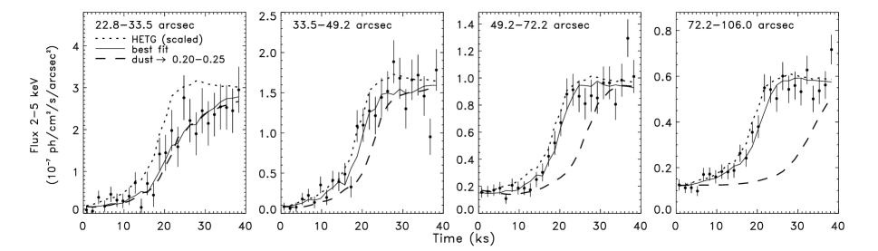
Figure 9.— Eclipse egress light curves from 2–5 keV for four annular regions (labeled in each panel). The model light curves for $D=5.7$ kpc are shown as solid curves. The dotted curves show the HETG light curve, and the dashed curve shows what the predicted light curves would be if the prominent dust cloud was shifted from $x=[0.00,0.05]$ to $x=[0.20,0.25]$.

Using the model flux history, we created model halo light curves for various energies, halo angles, and source distances, using the best-fit dust distribution as well as the three example dust distributions that are also consistent with the X-ray halo data. The final 2–5 keV single-scattered model light curves for the four annular regions are then derived by summing the energy bands and integrating over the annular regions, viz.

$$I_{1}(t,\Delta\theta)=\sum\limits_{i=0}^{14}\frac{1}{\pi(\theta_{2}^{2}-\theta_{1}^{2})}\int_{\theta_{1}}^{\theta_{2}}2\pi\theta I_{1}^{i}(t,\theta)d\theta,$$ (8)

where the superscript $i$ is a label that indicates the center of the 200 eV energy band at $(2.1+0.2i)$ keV, and $\theta_{1}$ and $\theta_{2}$ are the boundaries of each annular region.

Although the single-scattered halo light curves can be easily modeled, we must also account for multiply-scattered photons, as well as our ignorance of the specific form of the dust distribution (Fig. 5). Calculating the time dependence of multiply-scattered photons is computationally cumbersome (DT03). Fortunately, these photons comprise $\sim$10% of the total halo flux over the angles of interest (Fig. 3), so a rather simple treatment should be sufficient. Moreover, because the dust is concentrated at small $x$, the response of the halo to multiply-scattered photons should occur almost as rapidly as the response to single-scattered photons. Thus, to roughly account for multiply-scattered photons, we added 10% (the approximate value of $I_{2}/I_{1}$ over the angles of interest in the plateau phase observation) to the normalization of the single-scattered model light curves. We also allowed the normalization to vary by 10% when obtaining the fits.

To address the uncertainties in the dust distribution, we calculated model light curves for the best-fit distribution and for the three example distributions shown in Fig. 5. Although the general characteristics of the light curves (shape and normalization) for the different dust distributions were similar, subtle differences were present. The size of the differences in the light curves were about 7% $\pm$ 3% (relative to the model light curve for the best-fit distribution) at the beginning of the observation (and for the most part, independent of distance and angle), and 4% $\pm$ 1% at the end. Clearly, these measured differences only apply to the selected set of four potential dust distributions. In each case, however, the majority of the dust is located relatively close to the Sun, so the differences in the light curves from this set should provide a decent measure of the uncertainty in $I_{1}(t,\Delta\theta)$ due to the uncertainty in $\tilde{\rho}(x)$. We chose to account for the uncertainty in the dust distribution by adding $\sim$4%–7% (depending on differences in the model light curves as a function of time) to the intrinsic uncertainty of the halo light curves.

Figure 10.— Histogram of the best-fit distances to Cen X-3 from 2500 synthetic data sets. The distribution is fitted with the sum of two Gaussians. The standard deviation of the distribution is 1.45 kpc, and the 90% confidence level lower and upper limits, which are determined from the model of the distribution, are 2.1 kpc and 8.3 kpc, respectively.

Finally, the distance to Cen X-3 was obtained by fitting the model halo light curves for the four annular regions and for source distances between 3 kpc and 12 kpc in steps of 0.1 kpc to the observed light curves. For each distance, the $\chi^{2}$ statistic was used to determine the quality of the fit. Our results indicate that the distance to Cen X-3 is $5.7^{+0.5}_{-0.3}$ (${}^{+0.9}_{-0.7}$) kpc with 68% (90%) confidence (Figure 8). Note that we derive a more reasonable estimate of the distance uncertainty below.

The comparison of the measured halo light curves to the model fits for a source distance of 5.7 kpc (solid curves) is shown in Figure 9. Also shown is the model light curves if the $x=[0.00,0.05]$ dust cloud were moved to $x=[0.20,0.25]$. The halo light curves are therefore clearly consistent with most of the dust having a local origin.

Figure 11.— Similar to Fig. 8, but decreasing the width of the $x=[0.00,0.05]$ dust cloud to $\Delta x=0.01$ (while keeping the total amount of dust in the cloud constant by multiplying the normalization by 5) and trying each position within $x=[0.00,0.05]$.

Because the model light curves are not strictly linear in distance, $\Delta\chi^{2}$ may not be a legitimate estimator of the distance uncertainty (Fig. 8). A more reasonable estimate of the uncertainty can be obtained using Monte Carlo simulations. We accomplished this by simulating 2500 synthetic data sets, assuming the light curve models for $D=5.7$ kpc accurately describe physical reality, and assuming the measurement uncertainties are normally distributed. For each realization the best-fit distance is determined from the $\chi^{2}$ minimum. The resulting probability distribution of best-fit distances is presented in Figure 10, indicating that the uncertainty in distance based on $\Delta\chi^{2}$ is indeed too small, and that a more reasonable distance estimate to Cen X-3 is $5.7\pm 1.5$ $(^{+2.6}_{-3.6})$ kpc with 68% (90%) confidence. The 68% error limits were determined simply from the standard deviation of the distribution, and the 90% limits were determined by integrating over the model of the distribution, which is composed of the sum of two Gaussians.

Figure 12.— CO emission observed in the direction of Cen X-3 (Dame et al. 2001), with the two most prominent emission features labeled.

Another issue to address is the use of $\Delta x=0.05$ bins for the dust clouds. The uncertainty in the position of the dust within the $x=[0.00,0.05]$ cloud can have a significant effect on the model halo light curves. To test the effect of various dust positions for $x<0.05$ we calculated model light curves for the five positions with $\Delta x=0.01$ in $x<0.05$, maintaining a constant amount of dust in the cloud by increasing its normalization by a corresponding amount. For each of the five trial dust positions, the fit statistic was calculated at each distance (Fig. 11). The results are somewhat troubling, because although dust positions at $x<0.04$ do not greatly affect the implied distance, dust oriented at $x=[0.04,0.05]$ produce two local minima, with the best-fit distance becoming very small.

4.3. Comparison of Dust Distribution to CO Emission, Star Counts, and Interstellar Reddening

The dust distribution to Cen X-3 can be checked for consistency in a number of ways. Here we apply three methods. First, using the results of Dame et al. (2001), we can map the CO emission in the direction of Cen X-3, which presumably also traces the dust. The most prominent peak in the emission has a velocity of $-9.8$ km/s (Fig. 12). The kinematic distance to the CO responsible for this feature could be estimated from the rotation curve of the Galaxy, but because molecular clouds have a cloud-cloud dispersion of 4$-$5 km s^-1, kinematic distances for clouds with $|v|<10$ km s^-1 are not reliable; all that can be said is that CO emission has a relatively local origin (T. M. Dame, priv. comm.). Second, parallax measurements provide the spatial density of stars along the line of sight to Cen X-3. Using data from the Hipparcos Catalog, we created a histogram of the number of stars within 1$\fdg$25 of the line of sight (Figure 13). Of course, the parallax data are subject to certain selection effects. For one, stars at larger distances are less likely to be above the flux limit of the survey. On the other hand, a given solid angle corresponds to a larger volume of space at larger distances. Nevertheless, assuming star-forming regions are cospatial with regions of higher dust density, the histogram of star counts supports that conclusion that most of the dust is located at relatively small distances from the Sun. Finally, interstellar reddening data may be able to constrain the dust distribution. Marshall et al. (2006) modeled the interstellar extinction distribution in the Galaxy by comparing the infrared colors measured by the Two Micron All Sky Survey (2MASS; Cutri et al. 2003) to the colors from the Besançon model of the Galaxy (Robin et al., 2003). The resulting data for the Cen X-3 sightline, which shows the interstellar extinction ($A_{K_{\rm s}}$), are presented in Fig. 14 (top panel). The constant slope of $A_{K_{\rm s}}$ indicates that the dust is uniformly distributed between about 2 and 9 kpc. Because there are no data for $D\lesssim 2$ kpc, these interstellar reddening data cannot support or refute the claim for the local origin of the dust towards Cen X-3. However, by dividing the difference in extinction between neighboring bins by the distance between them, one can visualize the distribution of extinction elements along the sightline (Figure 14, bottom panel) for $D>2$ kpc. The results for this region of space are consistent with the dust being uniformly distributed, although we point out that the error bars allow for a slight increase in dust density for $D\gtrsim 3.5$ kpc, which is coincident with a slight increase in the upper limits to the size of the dust clouds shown in Fig. 5 for $x>0.65$.

Figure 13.— Histogram of the number of stars within 1$\fdg$25 of the line of sight to Cen X-3. Data are based on the Hipparcos Catalog. The fractional distance assumes a source distance of 5.7 kpc.

Figure 14.— Interstellar extinction ($A_{K_{\rm s}}$ and $\delta A_{K_{\rm s}}~{}{\rm kpc}^{-1}$) versus distance in the direction of Cen X-3 (centered 0$\fdg$13 away from the sightline). Data are from Marshall et al. (2006).

5. Discussion

In this paper, we have discovered that most of the dust along the line of sight to Cen X-3 is located relatively nearby the Sun, and that the distance to the binary system may be smaller than the commonly assumed distance of 8 kpc. Although our distance estimate is not particularly robust, we note that the best-fit distance and 8 kpc are only marginally inconsistent at the 68% confidence level, and the best-fit distance is consistent with 8 kpc at the 90% level.

Despite the uncertainty in the distance to Cen X-3, by all indications the dust along the line of sight to the system is heavily concentrated within about 300 pc of the Sun. Presumably, this dust is from the local Orion spur where the Sun resides. Not only do the X-ray halo measurements, the CO emission measurements, and the density of stars along the line of sight support this idea, but the halo light curves during egress clearly show a rapid response to changes in the point source flux (Fig. 9). In fact, model light curves for a uniform dust distribution (not shown), or for a distribution where the primary dust cloud is $x=[0.20,0.25]$, grossly misrepresent the data.

It is worth examining the difference between the energy dependence of the scattering optical depth predicted by the WD01 interstellar grain model, and the empirical curve describing Cen X-3 as well as data from Cyg X-1 and GX 13+1 (Fig. 4). Clearly, the shape of the WD01 curve and the Cen X-3 empirical curve differ substantially. One possible explanation for the discrepancy is our choice of $R_{V}=3.1$. After all, higher values of $R_{V}$ are observed in dense clouds, and we have found that most of the dust along the line of sight is located in a relatively small region of interstellar space. Yet this is not a viable explanation because the difference in the scattering optical depth for different values of $R_{V}$ (over 2–5 keV) is more in the normalization and not the shape of the curve. For a given optical depth at 2 keV, the increase in optical depth at 5 keV for $R_{V}=4.0$ ($R_{V}=5.5$) is 6–7% (14–15%), whereas a $\sim$60–80% difference is required to explain the energy dependence of $\tau_{\rm sca}$ in Cen X-3. Furthermore, the energy scaling of the scattering optical depth in Cyg X-1 and GX 13+1 more closely resembles the empirical curve for Cen X-3 than the WD01 model curve. In his comparison, Draine (2003) focused on the apparent differences between the predicted and measured values of $\tau_{\rm sca}/A_{V}$ for various X-ray sources, and not on the shape of the energy dependence. Our results, and those of Smith et al. (2002) and Yao et al. (2003), suggest that the WD01 model fails to accurately reflect the energy dependence of the scattering optical depth. Relative to the WD01 model, there appears to be less scattering at low energies, or alternatively, more scattering at high energies (due to uncertainties in the absolute normalization of the scattering optical depth) in Cyg X-1, GX 13+1, and Cen X-3.

6. Conclusions

1. The vast majority of the dust along the line of sight to Cen X-3 is located within 300 pc ($x<0.05$) of the Sun. The most likely location of the dust is the local Orion spur. However, we are not sensitive to dust located in the vicinity of Cen X-3 because data within $\sim$3″ of the central source are affected by pile-up.

2. The geometric distance to Cen X-3 is $5.7\pm 1.5$ kpc (68% confidence level), although this result is not valid if a large fraction of the dust is concentrated within $\Delta x=0.01$.

3. The energy scaling of the scattering optical depth predicted by the WD01 interstellar grain model does not accurately represent the results determined by X-ray halo studies of Cen X-3. Relative to the WD01 model, there appears to be less scattering at low energies or more scattering at high energies in Cyg X-1, GX 13+1, and Cen X-3.

Table 1Chandra/HETG PSF Parametrization

Energy Range	Normalization
(keV)	($10^{-5}~{}{\rm arcsec}^{-2}$)	$\Gamma$	$\chi^{2}_{\nu}$
1.0–1.2	9.9 $\pm$ 0.3 (3.6%)	2.62 $\pm$ 0.04	1.40
1.2–1.4	9.1 $\pm$ 0.4 (4.8%)	2.51 $\pm$ 0.05	0.99
1.4–1.6	7.8 $\pm$ 0.5 (6.4%)	2.48 $\pm$ 0.07	1.24
1.6–1.8	7.9 $\pm$ 0.6 (8.4%)	2.30 $\pm$ 0.09	1.92
1.8–2.0	8.7 $\pm$ 0.5 (5.9%)	2.48 $\pm$ 0.07	1.21
2.0–2.2	10.4 $\pm$ 0.6 (6.0%)	2.52 $\pm$ 0.07	1.44
2.2–2.4	9.0 $\pm$ 0.5 (6.8%)	2.44 $\pm$ 0.07	1.20
2.4–2.6	7.7 $\pm$ 0.7 (10.4%)	2.36 $\pm$ 0.12	2.20
2.6–2.8	7.8 $\pm$ 0.6 (8.9%)	2.12 $\pm$ 0.09	1.60
2.8–3.0	8.7 $\pm$ 0.7 (8.8%)	2.20 $\pm$ 0.10	1.21
3.0–3.2	9.6 $\pm$ 0.8 (9.7%)	2.24 $\pm$ 0.10	0.95
3.2–3.4	9.6 $\pm$ 0.8 (8.9%)	2.37 $\pm$ 0.10	1.12
3.4–3.6	10.0 $\pm$ 0.8 (8.7%)	2.13 $\pm$ 0.09	1.48
3.6–3.8	9.6 $\pm$ 0.8 (9.3%)	2.03 $\pm$ 0.09	1.23
3.8–4.0	10.5 $\pm$ 0.7 (7.4%)	1.97 $\pm$ 0.07	0.73
4.0–4.2	10.8 $\pm$ 0.8 (7.8%)	2.09 $\pm$ 0.07	1.16
4.2–4.6	11.8 $\pm$ 0.8 (7.2%)	2.00 $\pm$ 0.07	0.97
4.4–4.8	11.7 $\pm$ 0.8 (7.7%)	2.04 $\pm$ 0.07	1.29
4.6–4.8	11.6 $\pm$ 0.8 (7.3%)	1.92 $\pm$ 0.06	1.07
4.8–5.0	12.1 $\pm$ 0.8 (7.4%)	1.98 $\pm$ 0.06	1.83

Note. — PSF approximated by co-adding HETG observations of Her X-1 (ObsIDs 2749, 3821, 3822, 6149, & 6150) and PKS 2155-304 (ObsIDs 1014, 1705, 3167, 3706, 3708, 5173, 6926, 7291, 8380, & 8436). The PSF can be approximated by the function $S_{\rm PSF}(E,\theta)=A_{5}(E)\left(\theta/5\arcsec\right)^{-\Gamma(E)}$, where $A_{5}(E)$ is the normalization 5″ from the point source. Parameters apply from 3″ to 100″ from the central point source; an exponential cut-off is required for analysis of larger off-axis angles (Gaetz 2004).

For each observation, twenty different radial profiles were extracted in 200 eV energy bands from 1–5 keV using 40 logarithmically-spaced bins from 0$\farcs$492 (1 pixel) to 110″, with spatial filters applied to the readout transfer streak and the MEG and HEG diffraction pattern (offset by -4$\fdg$725 and 5$\fdg$235 from a line perpendicular to the readout) using rectangular regions 10 pixels wide. The radial profiles from each observation were then summed together and scaled to the total exposure time, resulting in images with units of [counts/s/pixel].

To account for differences in the detection efficiencies between the individual observations, separate instrument maps were created for each observation and energy band. Traditional instrument maps account for varying effective area and photon detection efficiencies across the CCD chip, but for PSF analysis it is only appropriate to use the effective area at the source position (Gaetz 2004). The aspect histograms of each observation were then used to project the instrument maps onto the plane of the sky, resulting in effective area maps accounting for bad rows on the CCD and the dither of the telescope. The dithered instrument maps, which showed deviations in the effective area at the source position of a few percent from observation to observation, were averaged by weighting each individual map by the number of counts in each energy and angular bin from the corresponding observation, correcting for the area of the spatial filters that were applied to the images. Radial profiles of the exposures maps were then created for the same annular regions as the profiles of the zeroth-order images, resulting in maps with units of [cm${}^{2}\times{\rm counts}/{\rm photons}$]. The final exposure-corrected radial profiles were then created by dividing the summed counts images by the averaged exposure map in each energy band. Using the summed spectrum, fluxes in each energy band were measured in units of [photons/cm²/s]. By dividing the exposure-corrected images by the fluxes in each energy band, we obtained normalized PSF profiles in 200 eV bands.

To each PSF profile (with background subtracted), we fit the function

$$S_{\rm PSF}(E,\theta)=A_{5}(E)\left(\frac{\theta}{5\arcsec}\right)^{-\Gamma(E)},$$ (1)

where $A_{5}(E)$ is the normalization 5″ from the central point source in units of flux fraction per square arcsecond. When modelling the PSF at larger off-axis angles (e.g., $\theta>100\arcsec$) it is necessary to include an exponential cut-off in the fitting function to account for the diffuse PSF wings (Gaetz 2004), but at smaller angles ($\theta<100\arcsec$) a simple power-law representation appears to be adequate. The final product that we obtained through this analysis is the energy- and angle-dependent fraction of the source flux comprising the PSF, as shown in Table 1. These results can be safely applied to Chandra/HETG observations 3″ to 100″ from the central source.

References

- Ash et al. (1999) Ash, T. D. C., Reynolds, A. P., Roche, P., Norton, A. J., Still, M. D., & Morales-Rueda, L. 1999, MNRAS, 307, 357
- Audley et al. (2006) Audley, M. D., Nagase, F., Mitsuda, K., Angelini, L., Kelley, R. L. 2006, MNRAS, 367, 1147
- Bildsten et al. (1997) Bildsten, L., et al. 1997, ApJS, 113, 367
- Burderi et al. (2000) Burderi, L., Di Salvo, T., Robba, N. R., La Barbera, A., & Guainazzi, M. 2000, ApJ, 530, 429
- Chandra (2007) Chandra X-Ray Center. 2007, Chandra Proposers’ Observatory Guide (ver. 10.0; Cambridge: Chandra X-Ray Cent.), http://cxc.harvard.edu/proposer/POG/html
- Clark et al. (1988) Clark, G. W., Minato, J. R., & Mi, G. 1988, ApJ, 324, 974
- Cutri et al. (2003) Cutri, R. M., Skrutskie, M. F., van Dyk, S., et al. 2003, Explanatory Supplement to the 2MASS All Sky Data Release
- Day & Stevens (1993) Day, C. S. R., & Stevens, I. R. 1993, ApJ, 403, 322
- Day & Tennant (1991) Day, C. S. R., & Tennant, A. F. 1991, MNRAS, 251, 76
- Dame et al. (2001) Dame, T. M., Hartmann, D., & Thaddeus, P. 1988, ApJ, 324, 248
- Dickey & Lockman (1990) Dickey, J. M., & Lockman, F. J. 1990, ARAA, 28, 215
- Draine (2003) Draine, B. T. 2003, ApJ, 598, 1026
- Draine & Tan (2003) Draine, B. T., & Tan, J. C. 2003, ApJ, 594, 347 (DT03)
- Gaetz (2004) Gaetz, T. 2004, Analysis of the Chandra On-Orbit PSF Wings (Cambridge: Chandra X-Ray Cent.), http://cxc.harvard.edu/cal/Hrma/psf/
- Hutchings et al. (1979) Hutchings, J. B., Cowley, A. P., Crampton, D., van Paradijs, J., & White, N. E. 1979, ApJ, 229, 1079
- Krzemiński (1974) Krzemiński, W. 1974, ApJ, 192, L135
- Marshall et al. (2006) Marshall, D. J.,Robin, A. C., Reylé, C., Schultheis, M., & Picaud, S. 2006, A&A, 453, 635
- Mathis et al. (1977) Mathis, J. S., Rumpl, W., & Nordsieck, K. H. 1977, ApJ, 217, 425
- Mathis & Lee (1991) Mathis, J. S., & Lee, C.-W. 1991, ApJ, 376, 490
- Nagase et al. (1992) Nagase, F., et al. 1992, ApJ, 396, 147
- Predehl et al. (2000) Predehl, P., Burwitz, V., Paerels, F., & Trümper, J. 2000, A&A, 357, L25
- Predehl & Schmitt (1995) Predehl, P., & Schmitt, J. H. M. M. 1995, A&A, 293, 889
- Priedhorsky & Terrell (1983) Priedhorsky, W. C., & Terrell, J. 1983, ApJ, 273, 709
- Rappaport & Joss (1983) Rappaport, S. A., & Joss, P. C. 1983, in Accretion Driven Stellar X-ray Sources, eds. W. H. G. Lewin and E. P. J. van den Heuvel, Cambridge University Press, 1
- Robin et al. (2003) Robin, A. C., Reylé, C., Derrière, S., & Picaud, S. 2003, A&A, 409, 523
- Smith & Dwek (1998) Smith, R. K., & Dwek, E. 1998, ApJ, 503, 831 (erratum 541, 512 [2000])
- Smith et al. (2002) Smith, R. K., Edgar, R. J., & Shafer, R. A. 2002, ApJ, 581, 562
- Suchy et al. (2008) Suchy, S., et al. 2008, ApJ, 675, 1487
- Takeshima et al. (1991) Takeshima, T., Dotani, T., Mitsuda, K., & Nagase, F. 1991, PASJ, 43, L43
- Thompson et al. (2006) Thompson, T. W. J., Rothschild, R. E., & Tomsick, J. A. 2006, ApJ, 650, 1063
- Trümper & Schönfelder (1973) Trümper, J., & Schönfelder, V. 1973, A&A, 25, 445
- Weingartner & Draine (2001) Weingartner, J. C., & Draine, B. T. 2001, ApJ, 548, 296 (WD01)
- Xiang et al. (2007) Xiang, J., Lee, J. C.; Nowak, M. A. 2007, ApJ, 660, 1309
- Yao et al. (2003) Yao, Y., Zhang, S. N., Zhang, X. L., & Feng, Y. X. 2003, ApJ, 594, L43
- Zubko et al. (2004) Zubko, V., Dwek, E., & Arendt, R. 2004, ApJS, 152, 211