Melting of persistent double–stranded polymers

Abstract

Motivated by recent DNA-pulling experiments, we revisit the Poland-Scheraga model of melting a double-stranded polymer. We include distinct bending rigidities for both the double-stranded segments, and the single-stranded segments forming a bubble. There is also bending stiffness at the branch points between the two segment types. The transfer matrix technique for single persistent chains is generalized to describe the branching bubbles. Properties of spherical harmonics are then exploited in truncating and numerically solving the resulting transfer matrix. This allows efficient computation of phase diagrams and force-extension curves (isotherms). While the main focus is on exposition of the transfer matrix technique, we provide general arguments for a reentrant melting transition in stiff double strands. Our theoretical approach can also be extended to study polymers with bubbles of any number of strands, with potential applications to molecules such as collagen.

I Introduction

Single-molecule micromanipulation techniques have opened up new opportunities for measurements and studies of polymers. Smith et al. pioneered Smith et al. (1992) stretching experiments of double-stranded DNA (dsDNA) and, along with others, observed that at high forces of about $65\mathrm{pN}$, DNA extends to $1.7$ times its contour lengthBensimon et al. (1995); Smith et al. (1996); Cluzel et al. (1996); Rief et al. (1999); Clausen-Schaumann et al. (2000). These investigators believe that the stretching transforms B-DNA, which is DNA in its natural state, to a new, extended state, named S-DNA. Modeling studies and simulations were carried out to characterize this putative new state of DNA.Konrad and Bolonick (1996); Kosikov et al. (1999); Lebrun and Lavery (1996) Subsequently, Storm and Nelson Storm and Nelson (2003) proposed a statistical model of DNA as a discrete persistent chain (DPC) with two monomer flavors of different lengths and stiffnesses, and fit their parameters successfully to experimental data. However, Williams, Rouzina, Bloomfield, and co-workers have argued on the basis of their own experiments that S-DNA is not a new state of the molecule, but merely DNA that is melted to two single-stranded DNA (ssDNA) fragments.Williams et al. (2002); Williams et al. (2001a, b); Rouzina and Bloomfield (2001a, b); Vladescu et al. (2005) Furthermore, they deem the aforementioned modeling and simulations of S-DNA as contradicting experimental data. Furthering this controversy, Cocco et al.Cocco et al. (2004) reexamine the experimental data and argue in favor of S-DNA, Whitelam et al.Whitelam et al. (2006) do so based on kinetics, while Piana Piana (2005) observes melting in simulations of short stretches of DNA.

In 1966 Poland and ScheragaPoland and Scheraga (1966) introduced a simple statistical model for the melting of the dsDNA to two ssDNA fragments, which has proved quite illuminating. In this model, configurations of partially melted DNA are represented by alternating segments of dsDNA, and denatured pairs of single strands forming ‘bubbles.’ To make the model analytically tractable, certain features of DNA such as excluded volume, bending rigidity, and sequence inhomogeneity are typically left out. With the later inclusion of excluded volume effects, the model is well suited for characterizing the nature of the melting transition, and its universality. For comprehensive (but older) reviews see Refs. Wartell and Benight (1985); Gotoh (1983); some newer results are described in, e.g. Ref. Kafri et al. (2002). More recently, the phase diagram of the model has been studied in the presence of a stretching force Hanke et al. (2008); Rudnick and Kuriabova (2007). This is important, since even the experiments disputing the formation of S-DNA at $65\mathrm{pN}$ do observe melting induced stretching at other forcesRief et al. (1999); Clausen-Schaumann et al. (2000). The effect of bending rigidity is still left out in the newer studies, making comparisons to experiment questionable. The aim of this paper is to facilitate the ongoing debate by providing a model that accounts for the bending rigidity of the polymer (while leaving out excluded volume effects).

While we hope that our results and phase diagrams provide an additional perspective into this system, our main accomplishment is the extension of the transfer matrix method used for a single persistent polymer (worm-like chain) to the melting of a double-stranded polymer. The remainder of the paper is an exposition of our method, and is organized as follows. The generalized Poland–Scheraga model with three types of bending rigidity is introduced in Sec. II.1, and the corresponding three contributions to transfer matrices are developed in Sec. II.2. As described in Sec. III, numerical results can be obtained by truncating the resulting transfer matrices in a basis of spherical harmonics. In particular, we provide phase diagrams (in force and temperature) and force–extension curves, along with the native (double stranded) fraction. We augment numerical results with physical explanations of the observed trends. In particular, we provide a rather general characterization of the slop of the phase boundary which explains the potential reentrant character of force induced melting. Various technical details of the calculation are relegated to the Appendices.

II Model

II.1 Energetics

Figure 1: A typical polymer configuration of our model, as depicted here, consists of segments R, solid arrows, which we imagine to be dsDNA, alternating with ‘bubbles’ B  made of two strands of ssDNA (light arrows). The two segment types have unit (monomer) lengths $|\vec{r}|$ or $|\vec{b}|$, and bending costs of $J_{R}$ or $J_{B}$, respectively. There is an additional bending constant $J_{J}$, at the branching points, and a weight $w_{J}=e^{\epsilon_{J}}$ for each joint. The energetic advantage (binding energy) of the R segments is represented by a weight $w_{R}=e^{\epsilon_{R}}$ per step.

As illustrated in Fig. 1, a typical configuration of our model polymer consists of an alternating sequence of native segments R, and locally molten pairs of strands forming a bubble B. Successive segments are indexed by $i$, and contain $N_{R,i}$ or $2N_{B,i}$ monomers, respectively. In the original Poland-Scheraga model Poland and Scheraga (1966), the R segments were treated as stiff ’r’ods. We treat these segments as semi-flexible chains, such that the energy of a segment of $N_{R,i}$ monomers is given by

$$\begin{split}-\beta E_{R}&=\sum_{j=1}^{N_{R}-1}\left(J_{R}~{}\hat{r}_{j}\cdot\hat{r}_{j+1}+\vec{r}_{j}\cdot\vec{f}\right)\\ &+\vec{r}_{N_{R}}\cdot\vec{f}+N_{R}\epsilon_{R}\quad.\end{split}$$ (1)

Here, $\vec{r}_{j}=|\vec{r}|\hat{r}_{j}$ is the displacement of the $j$’th ‘monomer’ of the segment, all of which have equal length, but may point in any direction. The coupling $J_{R}$ parameterizes the cost of bending neighboring monomers. The force $\vec{f}$ stretches the polymer, and $\epsilon_{R}$ is an additional contribution to the energy difference between a native R unit compared to the molted strands of B units. Note that (for each configuration, and discounting bending costs) the net energy difference between bound and unbound segments (the binding energy) is $k_{B}T(J_{R}+\epsilon_{R})$ per base-pair. (For ease of notation, the index $i$ denoting the $i$’th R segment has been dropped from all variables above.)

Similarly, the energy of a molten B region, described by $2N_{B,i}$ units $\vec{b}_{j}$ and $\vec{b}^{\prime}_{j}$ (for the two strands) is given by

$$\begin{split}-\beta E^{\prime}_{B}&=\sum_{j=1}^{N_{B}-1}\left(J_{B}~{}\hat{b}_{j}\cdot\hat{b}_{j+1}+\vec{b}_{j}\cdot\frac{\vec{f}}{2}\right)\\ &+\sum_{j=1}^{N_{B}-1}\left(J_{B}~{}\hat{b}^{\prime}_{j}\cdot\hat{b}^{\prime}_{j+1}+\vec{b}^{\prime}_{j}\cdot\frac{\vec{f}}{2}\right)\\ &+\vec{b}_{N_{B}}\cdot\frac{\vec{f}}{2}+\vec{b}^{\prime}_{N_{B}}\cdot\frac{\vec{f}}{2}\quad.\end{split}$$ (2)

Again, the implicit index $i$ numbering the $i$’th B segment has been omitted. The allowed configurations are constrained by $\vec{R}_{B}=\sum_{j=1}^{N_{B}}\vec{b}_{j}=\sum_{j=1}^{N_{B}}\vec{b}^{\prime}_{j}$, to ensure that the two branches of the bubble end at the same point. It is indeed this constraint (emphasized by the primed $E_{B}$) that allows distributing the energy cost of stretching by the force $\vec{f}$ symmetrically between the two branches.

Finally, there is a joint when the $N_{R,i}$’th (last) element of the $i$’th R segment branches into the first elements of the $i$’th B segment, to which we associate an energy

$$-\beta E_{J,RB}=J_{J}~{}\hat{r}_{N_{R}}\cdot\hat{b}_{1}+J_{J}~{}\hat{r}_{N_{R}}\cdot\hat{b}^{\prime}_{1}+\epsilon_{J}\quad.$$ (3)

Similarly at the point where the $i$’th B segment meets the $(i+1)$’th R segment, the energy is

$$-\beta E_{J,BR}=J_{J}~{}\hat{b}_{N_{B}}\cdot\hat{r}_{1}+J_{J}~{}\hat{b}^{\prime}_{N_{B}}\cdot\hat{r}_{1}+\epsilon_{J}\quad.$$ (4)

The overall energy of $M$ alternating R-B segments of sizes $\{N_{R,i},N_{B,i}\}$ is thus

$$\begin{split}&\beta E^{\prime}\left[N_{R,1},N_{B,1},N_{R,2},\cdots,N_{B,M}\right]=\\ &\sum_{i=1}^{M}\beta E_{R,i}+\beta E_{J,RB,i}+\beta E^{\prime}_{B,i}+\beta E_{J,BR,i}\quad.\end{split}$$ (5)

(The above formula applies to configurations which start with an R segment and end with a B segment. We expect the results for long polymers to be independent of the choice of boundary conditions.)

Computations are most easily performed in a grand canonical ensemble in which we sum over all possible polymer lengths, with a chemical potential $\mu/\beta$ per monomer. The grand partition function is then calculated from

$$\Gamma=\int_{\mathbf{S^{2}}}^{\prime}\sum_{N}e^{N\mu}\sum_{\{N_{R,i},N_{B,i}\}_{i=1}^{M}}e^{-\beta E^{\prime}\left[N_{R,1},\cdots,N_{B,M}\right]}\quad,$$ (6)

where $N=\sum_{i=1}^{M}N_{R,i}+N_{B,i}$ is the native polymer length. The integrations are over all directions of the monomer vectors $\hat{r}$, $\hat{b}$, and $\hat{b}^{\prime}$, provided that the bubble–closing constraints are satisfied. This can be ensured by inserting $\delta$-functions for each bubble segment, as

$$\delta\left(\sum_{j=1}^{N_{B,i}}\vec{b}_{j}-\sum_{j=1}^{N_{B,i}}\vec{b}^{\prime}_{j}\right)=\int\,\frac{d^{3}\vec{k}}{(2\pi)^{3}}\,e^{i(\sum\vec{b}_{j}-\sum\vec{b}^{\prime}_{j})\cdot\vec{k}}\quad.$$ (7)

II.2 Transfer Matrix Formulation

The one-dimensional character of the energy in Eq. (5) suggests a transfer matrix approach to the problem. This is indeed a standard tool for the study of semi-flexible chains Kramers and Wannier (1941); Storm and Nelson (2003); Wiggins et al. (2005); Yan and Marko (2003); Yan et al. (2005), but requires additional elaboration to treat the bubbles. Below, we shall develop step by step the contributions from the two segment types, and the joints in between, to the overall transfer matrix.

II.2.1 R segments

The Boltzmann weight in Eq. (6) involves a product of exponentials, similar in form to plane waves. Such exponentials can be expanded in a basis of spherical harmonics and Bessel functions, which then allows the integrations over the orientations $\hat{r}$, $\hat{b}$, and $\hat{b}^{\prime}$. For example, integrating over the unit vector $\hat{r}_{n}$ of an R segment yields

$$\begin{split}\int_{\mathbf{S^{2}}}e^{\cdots+J_{R}\hat{r}_{n-1}\cdot\hat{r}_{n}+J_{R}\hat{r}_{n}\cdot\hat{r}_{n+1}+\vec{r}_{n}\cdot\vec{f}+\epsilon_{R}+\mu+\cdots}\,d^{2}\hat{r}_{n}\\ =[\cdots Y_{\alpha}^{*}(\hat{r}_{n-1})]\left(T_{R}\right)_{\alpha,\beta}[Y_{\beta}(\hat{r}_{n+1})\cdots]\,,\end{split}$$ (8)

where summation over repeated indices is implied. Greek letters stand for elements of the angular momentum basis $|l,m\rangle$, e.g., $\alpha$ stands for $(l_{\alpha},m_{\alpha})$, and the transfer matrix elements are

$$\left(T_{R}\right)_{\alpha,\beta}=(4\pi)^{2}C_{\alpha,\bar{\beta},\gamma}i_{\beta}(J_{R})i_{\gamma}(|\vec{f}||\vec{r}|)Y_{\gamma}^{*}(\hat{f})~{}w_{R}~{}z~{}.$$ (9)

Here, $i_{\alpha}$ is the modified spherical Bessel function of the first kind of order $l_{\alpha}$; $C_{\alpha,\bar{\beta},\gamma}\equiv\int_{\mathbf{S^{2}}}Y_{\alpha}(\hat{r})Y_{\beta}^{*}(\hat{r})Y_{\gamma}(\hat{r})\,d^{2}\hat{r}$ is closely related to tabulated Gaunt coefficients, which can be expressed in terms of Wigner $3j$-symbols, see Appendix A; and each unit of an R segment carrier a fugacity $z=e^{\mu}$, and the binding weight $w_{R}=e^{\epsilon_{R}}$ defined earlier. To make the notation uniform and simple, a bar placed over an index of $C$, e.g. $C_{\alpha,\bar{\beta},\gamma}$, indicates that the corresponding spherical harmonic under the integral shall be complex conjugated. The repeated $\gamma$ index implies a (finite) sum. The expression simplifies if the force $\vec{f}$ is chosen to point along the $\hat{z}$ direction, in which case $(T_{R})_{\alpha,\beta}\propto\delta_{m_{\alpha},m_{\beta}}$. Note that the transfer matrix is asymmetric, as we have included $i_{\beta}(J_{R})$, but not $i_{\alpha}(J_{R})$ to avoid double-counting.

II.2.2 B segments

A similar computation for the two bubble strands yields two transfer matrices. These must be combined into one matrix to be usable in the later steps. Thus, the basis elements $|l,m\rangle$, $|l^{\prime},m^{\prime}\rangle$ are combined into one product basis element $|l,m\rangle\otimes|l^{\prime},m^{\prime}\rangle$ with one-letter abbreviation $\tilde{\alpha}\equiv(\alpha,\alpha^{\prime})=((l_{\alpha},m_{\alpha}),(l_{\alpha^{\prime}},m_{\alpha^{\prime}}))$, and

$$\begin{split}\iint_{\mathbf{S^{2}}}\frac{d^{3}\vec{k}}{(2\pi)^{3}}\begin{array}[]{l}d^{2}\hat{b}_{n}\\ d^{2}\hat{b}^{\prime}_{n}\end{array}\begin{array}[]{l}e^{\cdots+J_{B}\hat{b}_{n-1}\cdot\hat{b}_{n}+J_{B}\hat{b}_{n}\cdot\hat{b}_{n+1}+\vec{b}_{n}\cdot\frac{\vec{f}}{2}+i\vec{b}_{n}\cdot\vec{k}+\cdots}\\ e^{\cdots+J_{B}\hat{b}^{\prime}_{n-1}\cdot\hat{b}^{\prime}_{n}+J_{B}\hat{b}^{\prime}_{n}\cdot\hat{b}^{\prime}_{n+1}+\vec{b}^{\prime}_{n}\cdot\frac{\vec{f}}{2}-i\vec{b}^{\prime}_{n}\cdot\vec{k}+\cdots}\end{array}z\\ =\int\frac{d^{3}\vec{k}}{(2\pi)^{3}}\begin{array}[]{l}\left[\cdots Y_{\alpha}^{*}(\hat{b}_{n-1})\times\right]\\ \left[\cdots Y_{\alpha^{\prime}}^{*}(\hat{b}^{\prime}_{n-1})\times\right]\end{array}(T_{B}(\vec{k}))_{\tilde{\alpha},\tilde{\beta}}\begin{array}[]{l}\left[\times Y_{\beta}(\hat{b}_{n+1})\cdots\right]\\ \left[\times Y_{\beta^{\prime}}(\hat{b}^{\prime}_{n+1})\cdots\right]\end{array}\\ \end{split}\,,$$ (10)

where

$$\begin{split}(T_{B}(\vec{k}))_{\tilde{\alpha},\tilde{\beta}}=z\int Y_{\alpha}(\hat{b})e^{\vec{b}\cdot\frac{\vec{f}}{2}+i\vec{b}\cdot\vec{k}}Y_{\beta}^{*}(\hat{b})(4\pi)i_{\beta}(J_{B})\,d^{2}\hat{b}\\ \times\int Y_{\alpha^{\prime}}(\hat{b}^{\prime})e^{\vec{b}^{\prime}\cdot\frac{\vec{f}}{2}-i\vec{b}^{\prime}\cdot\vec{k}}Y_{\beta^{\prime}}^{*}(\hat{b}^{\prime})(4\pi)i_{\beta^{\prime}}(J_{B})\,d^{2}\hat{b}^{\prime}\quad.\\ \end{split}$$ (11)

This transfer matrix is, in general, very big. If the spherical harmonic basis elements are cut off at some $l_{\text{max}}$ for numerical evaluation, there are $(l_{\text{max}}+1)^{2}$ basis elements to consider since $m\in\{-l,\cdots,l\}$ for each $0\leq l\leq l_{\text{max}}$. This means that there are $((l_{\text{max}}+1)^{2})^{2}$ product basis elements, which is the number of rows or columns of the transfer matrix $T_{B}(\vec{k})$! With a little trick this big matrix can be reduced to block diagonal form with the biggest submatrix having size $(l_{\text{max}}+1)^{2}$:

Consider the first integral in Eq. (11) and let $\vec{v}=i\vec{k}+{\vec{f}}/{2}$ indicate the vector in the exponent. One can rotate the complex vector $\vec{v}$ into the $\hat{z}$-direction, such that

$$\begin{split}&(4\pi)\int Y_{\alpha}(\hat{b})e^{\vec{b}\cdot\vec{v}}Y_{\beta}^{*}(\hat{b})i_{\beta}(J_{B})\,d^{2}\hat{b}=\\ &(4\pi)\,\mathcal{D}_{\alpha,\mu}\left(\int Y_{\mu}(\hat{b})e^{\vec{b}\cdot|\vec{v}|\hat{z}}Y_{\nu}^{*}(\hat{b})i_{\nu}(J_{B})\,d^{2}\hat{b}\right)\mathcal{D}_{\nu,\beta}^{-1}=\\ &(4\pi)^{2}\mathcal{D}_{\alpha,\mu}\left(C_{\mu,\bar{\nu},\gamma}i_{\nu}(J_{B})i_{\gamma}(|\vec{v}||\vec{b}|)Y_{\gamma}^{*}(\hat{z})\right)\mathcal{D}_{\nu,\beta}^{-1}~{},\\ \end{split}$$ (12)

where $\mathcal{D}(\phi,\theta,0)$ is the rotation matrix (Wigner-D matrix or Wigner-D function) for quantum mechanical angular momentum states. The spherical coordinate angles $\theta$ (from the $z$-axis) and $\phi$ (from the $x$-axis) are the angles by which the $\hat{z}$-direction rotates into the $\vec{v}$-direction. The rotation matrices are usually parametrized by Euler angles. The first Euler angle corresponds to $\phi$, the second to $\theta$, and the third to zero. Since $\vec{v}$ is complex, the angles of rotation are complex and $|\vec{v}|$, which is the usual Euclidean norm of $\vec{v}$, is also complex, as $|\vec{v}|^{2}\equiv\vec{v}\cdot\vec{v}=f^{2}/4-k^{2}+i\vec{k}\cdot\vec{f}$. Note that $i_{\beta}(J_{B})$ in the first line can be replaced by $i_{\nu}(J_{B})$ because $i_{\beta}$ only depends on $l_{\beta}$ while $\mathcal{D}$ only mixes states with the same total angular momenta, i.e. $\mathcal{D}_{\nu,\beta}\propto\delta_{l_{\nu},l_{\beta}}$. Although the dependence on $\vec{k}$ is now both in $\mathcal{D}$ as well as in $i_{\gamma}$, the problem is computationally much simpler since $C_{\mu,\bar{\nu},\gamma}Y_{\gamma}^{*}(\hat{z})\propto\delta_{m_{\mu},m_{\nu}}$.

II.2.3 Joints

Similar manipulations lead to transfer matrices at the branching points of

$$\begin{split}(T_{J,RB})_{\alpha,\tilde{\beta}}&=(4\pi)^{3}C_{\alpha,\gamma,\bar{\xi}}C_{\bar{\beta},\bar{\beta}^{\prime},\xi}i_{\gamma}(|\vec{f}||\vec{r}|)Y_{\gamma}^{*}(\hat{f})\\ &\times i_{\beta}(J_{J})i_{\beta^{\prime}}(J_{J})~{}w_{R}~{}w_{J}~{}z~{},\end{split}$$ (13)

and

$$\begin{split}(T_{J,BR})_{\tilde{\alpha},\beta}&=(4\pi)^{2}C_{\bar{\alpha},\bar{\alpha}^{\prime},\xi}C_{\beta,\gamma,\bar{\xi}}i_{\gamma}(|\vec{f}||\vec{r}|)Y_{\gamma}^{*}(\hat{f})\\ &\times\frac{i_{\alpha}(J_{J})i_{\alpha^{\prime}}(J_{J})}{i_{\alpha}(J_{B})i_{\alpha^{\prime}}(J_{B})}i_{\beta}(J_{R})~{}w_{R}~{}w_{J}~{}z~{}.\end{split}$$ (14)

Once more the lack of symmetry between the two cases reflects our choice of including the bending energy from the next (but not the previous) segment in the transfer matrix. The absence of the joint energy $J_{J}$ greatly simplifies the problem, as the R  and B  segments can then be treated independently. This happens because $i_{\alpha}(0)=0$ unless $l_{\alpha}=0$.

Combining these expressions, we can express the partition function $\Gamma$ in Eq. (6) in terms of the transfer matrices (the irrelevant prefactors have been omitted), as

$$\begin{split}\Gamma\propto&\left.\sum_{M=1}^{\infty}\left[\left(\sum_{i=0}^{\infty}T_{R}^{i}\right)T_{J,RB}\left(\int\frac{d^{3}\vec{k}}{(2\pi)^{3}}\sum_{i=2}^{\infty}T_{B}^{i}\,\right)T_{J,BR}\right]^{M}\right|_{0,0}\\ &=\left.\frac{\Gamma_{R}T_{J,RB}\Gamma_{B}T_{J,BR}}{1-\Gamma_{R}T_{J,RB}\Gamma_{B}T_{J,BR}}\right|_{0,0},\end{split}$$ (15)

where

$$\Gamma_{R}=(1-T_{R})^{-1},$$ (16)

and

$$\Gamma_{B}=\int\frac{d^{3}\vec{k}}{(2\pi)^{3}}\,\frac{T_{B}(\vec{k})^{2}}{1-T_{B}(\vec{k})}\,.$$ (17)

III Results

In the grand canonical ensemble the average length of the polymer is given by $\langle N\rangle=\partial_{\mu}\log(\Gamma)=z\partial_{z}\log(\Gamma)$. We are interested in the limit of very long polymers, where $\langle N\rangle\to\infty$. This limit is obtained for a specific choice of the fugacity $z=e^{\mu}$, such that:

1. There are infinitely many repetitions of native (R) and molten (B) segments. This occurs for a value of $z$ such that the largest eigenvalue of $[\Gamma_{R}T_{J,RB}\Gamma_{B}T_{J,BR}](z)$ equals $1$.

2. The size of an individual bubble diverges. In this case the singularity arises from $\partial_{z}\Gamma_{B}(z)$.

3. The hypothetical possibility of an infinitely long native (R) segment does not arise, as $\partial_{z}\Gamma_{R}(z)$ only diverges for values of $z$ that already cause one of the previous two cases to occur.

As in the Poland-Scheraga model Poland and Scheraga (1966), case (1) corresponds to a partially melted double strand (mixed phase of R and B segments), while case (2) corresponds to a fully melted state comprised of one bubble (bubble phase).

III.1 Phase Diagram

A phase transition between the two phases occurs when there are both infinitely many repetitions of R and B segments, and the average bubble size diverges. Since our model has 6 parameters, we have to select appropriate subspaces for the display of phase diagrams. We choose to regard the bending energies $J_{R}$, $J_{B}$, $J_{J}$, and the joint Boltzmann weight $w_{J}=e^{\epsilon_{J}}$ as parameters, and display the phase diagrams as a function of the force $f$ and the dimensionless energy $\epsilon_{R}=\log(w_{R})$. The latter may be regarded as a stand-in for an inverse temperature, since it is related to an actual energy after division by $k_{B}T$. (As discussed following Eq. (1), negative values of $\epsilon_{R}(f)$ do not pose a problem, as the actual binding energy is $k_{B}T(J_{R}+\epsilon_{R})$.)

Some typical phase boundaries $\epsilon_{R}(f)$ are presented in Fig. 2. We used the Mathematica software package on an Intel Pentium 3 GHz desktop computer to obtain the phase diagrams, each of which took a few hours of computational time when we included partial waves up to $l=1$ in the bubble (B) partition functions, and $l=5$ in the native (R) partition functions. It should be possible to reduce the computational time significantly by using more appropriate software. The truncation of the transfer matrices at these partial waves was justified considering the small bending parameters chosen for the bubbles and the joints.

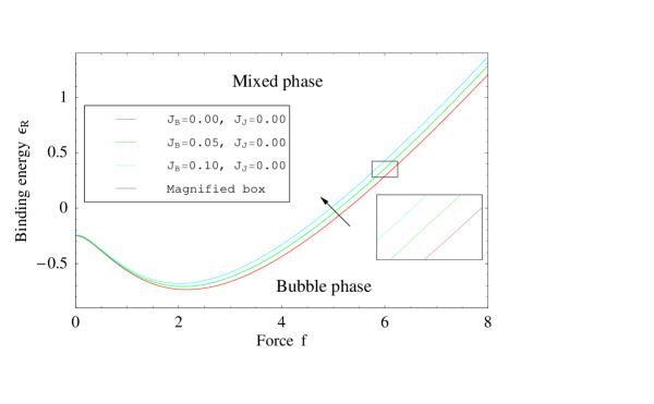
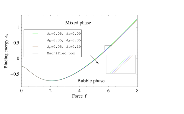
Figure 2: The phase boundaries $\epsilon_{R}(f)$ separate the partially melted R-B phase (above the line) from the fully melted bubble phase (below the line), for various combinations of $J_{B}$ and $J_{J}$. Top: The bubble stiffness $J_{B}$ is increased. Bottom: The joint stiffness $J_{J}$ is increased. In both plots, the arrow indicates the direction in which the phase boundary moves. In all curves $|\vec{r}|=1.0,\,|\vec{b}|=1.7,\,J_{R}=5.0$, and $\epsilon_{J}=1.0$.

Each solid curve depicts the phase boundary for a particular choice of parameters. All curves correspond to rather stiff R-segments with $J_{R}=5.0$, but for different choices of the bending bending parameters $J_{B}$ and $J_{J}$. The upper portion of each figure corresponds to the partially melted native state, which contains both R  and B  segments. There is no native R segment left in the lower portion, and the polymer is a single bubble below the phase transition line. The lowest curve in the top figure (red in the online version) corresponds to no bending in the bubble or vertex; $J_{B}=J_{J}=0$. As we increase $J_{B}$ to larger values of 0.05 and 0.1 in the top figure (green and cyan, online), the bubble phase becomes more stable. (The phase boundary moves up as indicated by the arrow.) If we now fix $J_{B}=0.05$, and increase $J_{J}$ to values of 0.05 and 0.1 in the bottom figure (blue and brown online) we find that $\epsilon_{R}(f)$ moves down, as indicated by the arrow. The mixed phase is stabilized by stiffening the joints between R- and B-segments.

Several features of these phase diagrams are now commented on in more detail.

III.1.1 Explanation of the trends in phase diagrams

With our choice of parameters, increasing the value of any stiffness parameter $J$, makes the corresponding segment (or joint) more favorable. This is because the corresponding Boltzmann weights are monotonically increasing functions of $J$ (as are the modified spherical Bessel functions $i_{\alpha}(J)$). For example, for a bubble segment the overall weight increases with $J_{B}$, despite the fact that there are fewer configurations (and hence reduced) entropy for the stiffened and stretched bubble. These trends are further magnified at larger force as the stretched segments gain even more weight by aligning to the force, as can be easily seen in Fig. 2.

III.1.2 Reentrance & the phase boundary at low and high forces

An interesting feature of the phase boundary in Fig. 2 is its reentrance, namely for certain choices of $\epsilon_{R}$ ($-0.8<\epsilon_{R}<-0.2$) the mixed R-B phase is stable at intermediate values of the force, but melts at both weak and strong force. This reentrance is also present in another model of denaturation which incorporates excluded volume effects in the bubbles, but no bending rigidity Hanke et al. (2008).

This feature can be explained by examining the limiting behaviors of the phase boundary at small and large $f$. For large $f$, the polymer (whether in native or denatured state) is stretched along the direction of the force. The contribution from entropy is relatively small in this limit, and one can estimate the location of the phase boundary by comparison of energies: The energy of a fully stretched rod segment is $J_{R}+\epsilon_{R}+f|\vec{r}|$ per base-pair. If the two strands are separated the energy changes to $2J_{B}+f|\vec{b}|$. The transition occurs for $\epsilon_{R}\approx 2J_{B}-J_{R}+(|\vec{b}|-|\vec{r}|)f$, which has a positive slope since B strands have longer monomers and are favored by the force.

As shown in Appendix B, this argument can be made more rigorous and extended to all cases where the contribution from the joints can be ignored. In such cases the slope of the phase boundary is given by $\partial_{f}\epsilon_{R}={\langle L_{B}\rangle}/{\langle N_{B}\rangle}-{\langle L_{R}\rangle}/{\langle N_{R}\rangle}$, where $\frac{\langle L_{X}\rangle}{\langle N_{X}\rangle}$ denotes the average length per monomer, calculated for each segment type (B segment or R segment) treated separately.

At zero force, the average end-to-end extension of each segment, $\langle L_{X}\rangle$, is zero by symmetry. The extension for small $f$ is linear, with a force constant (susceptibility) that is easily related to the variance of the end-to-end extension at $f=0$. Since the change in free energy is proportional to $f^{2}$, the phase boundary is also quadratic in this limit. In the absence of joint stiffness, the curvature of the transition line can be related to the difference in susceptibilities by $\partial_{f}^{2}\epsilon_{R}={\langle L_{B}^{2}\rangle_{c}}/{\langle N_{B}\rangle}-{\langle L_{R}^{2}\rangle_{c}}/{\langle N_{R}\rangle}$, see Appendix B for a derivation. Here, ${\langle L_{X}^{2}\rangle_{c}}/{\langle N_{X}\rangle}$ denotes the variance in length of rods or bubbles per monomer, computed for one rod segment or one bubble segment subject to the same fugacity and force as for the whole molecule. Since it is easier to rotate and align the more rigid R segments in the direction of the force, their gain from the force is larger, and small force favors the native double-stranded phase.

The reentrance in the phase diagram of reference Hanke et al. (2008), mentioned in the first paragraph of this subsection, can be explained with these expressions as well. In this paper different behaviors are obtained as a function of a parameter $A$, which determines how statistically favored joints are. They observe a reentrant phase diagram for $A=0.01$ (disfavoring joints) but not for $A=1$ (many joints). The variance per monomer in the lengths of the bubbles is roughly constant (${\langle L_{B}^{2}\rangle_{c}}\propto{\langle N_{B}\rangle}$ as in a random walk), but for stiff rods the variance grows as the average size (${\langle L_{R}^{2}\rangle_{c}}\propto{\langle N_{R}\rangle^{2}}$ as in a directed walk). For small $A$, there are few joints and longer rods just after the phase transition into the mixed bubble–rod phase, making the variance per monomer large. According to the above formula for $\partial_{f}^{2}\epsilon_{R}$ this leads to reentrance. Note that excluded volume effects do not substantially modify this argument.

Williams et al. experimentally observe (Figure 5 of Ref. Williams et al. (2002)) a reentrance in the phase boundary when they fit their data to a simple model. Unfortunately, the area of interest is merely extrapolated and the transition is not probed at high enough temperatures and low forces ($\approx 90^{\circ}$) to unambiguously verify reentrance.

III.2 Force–Extension Isotherms

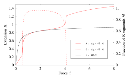
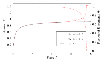
Figure 3: Comparison of the extension curves $X(f)=\langle L_{z}\rangle/\langle N|\vec{r}|\rangle$ (solid lines) for a double-stranded polymer, and a single stranded wormlike chain. The top panel corresponds to a case where melting is reentrant ($\epsilon_{R}=-0.4$), while there is a single denaturation transition in the bottom panel for $\epsilon_{R}=1.0$ (cf. Fig. 2). The fraction of native (double stranded) polymer, $\Theta\equiv\langle N_{r}\rangle/\langle N\rangle$, is indicated by dashed lines. All curves correspond to $J_{B}=J_{J}=0$, $|\vec{r}|=1.0,\,|\vec{b}|=1.7,\,J_{R}=5.0$, and $\epsilon_{J}=1.0$ for the double strands.

An important probe of phase behavior comes from the force–extension curves, in which the end-to-end distance of the polymer is measured as a function of increasing force. Without loss of generality and to simplify calculations, these curves are obtained for $J_{B}=J_{J}=0$ (with $J_{R}=5.0,\,\epsilon_{J}=1.0$). For comparison, we also plot the curves corresponding to the pure worm-like chain (WLC) model in black (containing only R segments for $w_{J}=0$). The plotted ‘extension’ is the average length along the force direction, made intensive and dimensionless by dividing by the number of monomers $\langle N\rangle$, and the monomer length $|\vec{r}|$ of the R segment, i.e.

$$X=\frac{\langle L_{z}\rangle}{\langle N|\vec{r}|\rangle}=\frac{\partial_{f}\Gamma}{\partial_{\mu}\Gamma}=-\frac{d}{df}\left(\ln z\right)\big{|}_{\Gamma=\infty}.$$ (18)

The two panels in Fig. 3 were selected to correspond to parameters with (top) and without (bottom) reentrant melting. (Consider horizontal lines in Fig. 2 for $\epsilon_{R}=-0.4$ and $\epsilon_{R}=1.0$, respectively.) In both cases, the force-extension curves for the double-stranded polymer track the behavior of the worm-like chain closely in the mixed R-B phase, but deviate significantly in the denatured phases; most pronouncedly for the re-entrant transition.

As mentioned earlier, current experiments indicate that the WLC model describes the extension of DNA accurately for small applied forces, but fails at large forces due to the appearance of an over-stretched region. In Fig. 4 we probe the corresponding region in more detail for our model, exploring the effect of bending rigidities (for $\epsilon_{R}=1.0$ with a single transition). The top panel depicts the effect of increasing the bubble stiffness $J_{B}$, which makes the transition region appear sharper. Increasing the joint stiffness $J_{J}$ (bottom panel) has the opposite effect.

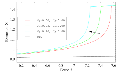
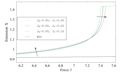
Figure 4: Detailed view of the dimensionless extension $X=\langle L_{z}\rangle/\langle N|\vec{r}|\rangle$ as a function of the force $f$, close to the phase transition, for various combinations of $J_{B}$ and $J_{J}$. Top – The bubble stiffness $J_{B}$ is increased. Bottom – The joint stiffness $J_{J}$ is increased. In both plots, the arrows indicate the direction the extension curve moves. In all curves $|\vec{r}|=1.0,\,|\vec{b}|=1.7,\,J_{R}=5.0$, and $\epsilon_{J}=1.0$.

An interesting feature of the bottom panel is that the trends in $X(f)$ are not monotonic in $J_{J}$, decreasing the extension for weaker force, and increasing it for larger force, leading to a crossing point in between. The reader should note that we have taken $\epsilon_{J}=1.0$ in all curves, making the joints favorable and common. This choice is made to exaggerate the effect of the joint bending for display, as well as to broaden the phase transition in Fig. 4, thus highlighting the features of our model. A more realistic value, namely $\epsilon_{J}$ small or negative, gives qualitatively similar results.

III.3 $\Theta$: Native (R) fraction

Figure 3 also includes the native fraction $\Theta$ as a function of $f$, depicted by the dashed curves. This is defined as the fractional amount of R segments in the polymer, which can be computed from

$$\Theta\equiv\frac{\langle N_{R}\rangle}{\langle N\rangle}=\frac{w_{R}\partial_{w_{R}}\Gamma}{z\partial_{z}\Gamma}.$$ (19)

Note that $\Theta$ goes to zero continuously on approaching the bubble phase, underscoring the second order nature of the phase transition. It approaches zero rapidly, but in a linear fashion. This is because the phase transition in our model belongs to the same universality class as the classic Poland-Scheraga model Poland and Scheraga (1966). The addition of bending rigidity is irrelevant close to the phase transition, and excluded volume effects (which do modify the universality Kafri et al. (2002); Hanke et al. (2008)) are not included in our model.

IV Discussion

We have introduced a formalism to address the role of bending rigidity in the denaturation of double-stranded polymers, DNA providing a prime example. There has been some controversy on interpreting experimental results for melting of DNA, or its denaturation by force. There is strong theoretical indication that the melting of a uniform double-stranded polymer should be discontinuous due to excluded volume effects Kafri et al. (2002). The discontinuity may be masked in experiments because of the inherent inhomogeneity of DNA Rudnick and Kuriabova (2007); Tang and Chaté (2001), or by finite-size effects. The rigidity of DNA should play an important role in the latter, as longer persistent segments are less susceptible to fluctuations and excluded-volume effects. It is thus necessary that comparison of models to experiment should include the effect of rigidity, as we have attempted here. More generally, our formalism can be extended to decribe the unravelling of any number of strands, for example from 1 to 3 in the case of collagen Thompson et al. (2001); Gutsmann et al. (2004).

Appendix A Gaunt coefficients

The Gaunt coefficients are defined as

$$C_{\alpha,\beta,\gamma}\equiv\int_{\mathbf{S^{2}}}Y_{\alpha}(\hat{r})Y_{\beta}(\hat{r})Y_{\gamma}(\hat{r})\,d^{2}\hat{r}\quad,$$ (20)

where $Y_{\alpha}$ is the spherical harmonic with indices $(l_{\alpha},m_{\alpha})$. If a bar is put on top of an index of $C$, the corresponding spherical harmonic in the integrand is complex conjugated. The relation

$$Y_{l,m}^{*}=(-1)^{m}Y_{l,-m}\,,$$ (21)

can be used to relate a modified Gaunt coefficient with barred indices to one without barred indices. A well-known expression for the Gaunt coefficient in terms of Wigner $3j$-symbols is Weisstein

$$\begin{split}C_{\alpha,\beta,\gamma}&=\sqrt{\frac{(2l_{\alpha}+1)(2l_{\beta}+1)(2l_{\gamma}+1)}{4\pi}}\\ &\times\begin{pmatrix}l_{\alpha}&l_{\beta}&l_{\gamma}\\ 0&0&0\\ \end{pmatrix}\begin{pmatrix}l_{\alpha}&l_{\beta}&l_{\gamma}\\ m_{\alpha}&m_{\beta}&m_{\gamma}\\ \end{pmatrix}.\end{split}$$ (22)

Using the properties of the Wigner $3j$-symbols one can restrict and simplify the sums appearing in the partition function.

Appendix B Slope of the phase boundary

When the joint stiffness $J_{J}$ vanishes, the partition function matrices $\Gamma_{R}$ and $\Gamma_{B}$ in Eqs. (16) and (17) reduce to real-valued functions. As discussed in the Sec. III, two conditions have to be met at the phase transition, $\Gamma_{B}\Gamma_{R}=1$ and $\partial_{z}\Gamma_{B}=\infty$, where in the former equation all multiplicative factors from the joints are absorbed in either of the two partition functions. Together, these two conditions set the value of $\mu=\log(z)$ and $\epsilon_{R}=\log(w)$ along the phase boundary. All manipulations below are then performed as the boundary point is changed by varying the force $f$.

Noting that, the first condition is equivalent to

$$\log\Gamma_{B}(\mu,f)+\log\Gamma_{R}(\mu,f,\epsilon_{R})=0\quad,$$ (23)

its variations are obtained, by taking one total derivative with respect to $f$, as

$$\begin{split}0=&\partial_{f}\log\Gamma_{B}+\partial_{\mu}\log\Gamma_{B}\,\partial_{f}\mu+\\ &\partial_{f}\log\Gamma_{R}+\partial_{\mu}\log\Gamma_{R}\,\partial_{f}\mu+\partial_{\epsilon_{R}}\log\Gamma_{B}\,\partial_{f}\epsilon_{R}\\ =&\langle L_{B}\rangle+\langle N_{B}\rangle\partial_{f}\mu+\\ &\langle L_{R}\rangle+\langle N_{R}\rangle(\partial_{f}\mu+\partial_{f}\epsilon_{R}).\end{split}$$ (24)

From the second condition we get

$$\left.\partial_{f}\mu\right|_{\partial_{\mu}\Gamma_{B}=\infty}=-\frac{\partial_{f}\partial_{\mu}\Gamma_{B}}{\partial_{\mu}\partial_{\mu}\Gamma_{B}}=-\frac{\langle L_{B}N_{B}\rangle}{\langle N_{B}^{2}\rangle}.$$ (25)

But because the condition $\partial_{\mu}\Gamma_{B}=\infty$ of infinite bubble length is the same as $\partial_{\mu}\log\Gamma_{B}=\infty$, one can equivalently express

$$\left.\partial_{f}\mu\right|_{\partial_{\mu}\log\Gamma_{B}=\infty}=-\frac{\partial_{f}\partial_{\mu}\log\Gamma_{B}}{\partial_{\mu}\partial_{\mu}\log\Gamma_{B}}=-\frac{\langle L_{B}N_{B}\rangle_{c}}{\langle N_{B}^{2}\rangle_{c}}\,,$$ (26)

where the subscript ‘c’ indicates a cumulant in place of a moment. From combining both expressions it follows that

$$\left.\partial_{f}\mu\right|_{\partial_{\mu}\Gamma_{B}=\infty}=-\frac{\langle L_{B}\rangle}{\langle N_{B}\rangle}.$$ (27)

Plugging this result into Eq. (24), one obtains

$$\partial_{f}\epsilon_{R}=\frac{\langle L_{B}\rangle}{\langle N_{B}\rangle}-\frac{\langle L_{R}\rangle}{\langle N_{R}\rangle}.$$ (28)

Note that at zero force all averages with only one $L_{B}$ or $L_{R}$ are zero by symmetry. Taking another total derivative of Eq. (24), and dropping the terms that vanish for this reason, one finds that at $f=0$

$$\begin{split}0=&\langle L_{B}^{2}\rangle_{c}+\langle N_{B}\rangle\partial_{f}^{2}\mu+\\ &\langle L_{R}^{2}\rangle_{c}+\langle N_{R}\rangle(\partial_{f}^{2}\mu+\partial_{f}^{2}\epsilon_{R}).\end{split}$$ (29)

Taking another derivative of $\mu$ in Eq. (27) one finds (for $f=0$)

$$\left.\partial_{f}^{2}\mu\right|_{\partial_{\mu}\Gamma_{B}=\infty}=-\frac{\langle L_{B}^{2}\rangle}{\langle N_{B}\rangle}.$$ (30)

Combining Eqs. (29) and (30) the desired slope at $f=0$ is obtained as

$$\partial_{f}^{2}\epsilon_{R}=\frac{\langle L_{B}^{2}\rangle_{c}}{\langle N_{B}\rangle}-\frac{\langle L_{R}^{2}\rangle_{c}}{\langle N_{R}\rangle}.$$ (31)

References

- Smith et al. (1992) S. B. Smith, L. Finzi, and C. Bustamante, Science 258, 1122 (1992).
- Bensimon et al. (1995) D. Bensimon, A. J. Simon, V. Croquette, and A. Bensimon, Physical Review Letters 74, 4754 (1995).
- Smith et al. (1996) S. B. Smith, Y. Cui, and C. Bustamante, Science 271, 795 (1996).
- Cluzel et al. (1996) P. Cluzel, A. Lebrun, C. Heller, R. Lavery, J.-L. Viovy, D. Chatenay, and F. Caron, Science 271, 792 (1996).
- Rief et al. (1999) M. Rief, H. Clausen-Schaumann, and H. E. Gaub, Nature Structural Biology 6, 346 (1999).
- Clausen-Schaumann et al. (2000) H. Clausen-Schaumann, M. Rief, C. Tolksdorf, and H. E. Gaub, Biophysical Journal 78, 1997 (2000).
- Konrad and Bolonick (1996) M. W. Konrad and J. I. Bolonick, J. Am. Chem. Soc. 118, 10989 (1996).
- Kosikov et al. (1999) K. M. Kosikov, A. A. Gorin, V. B. Zhurkin, and W. K. Olson, J. Mol. Biol. 289, 1301–1326 (1999).
- Lebrun and Lavery (1996) A. Lebrun and R. Lavery, Nucleic Acids Res. 24, 2260 –2267 (1996).
- Storm and Nelson (2003) C. Storm and P. C. Nelson, Phys. Rev. E 67, 051906 (2003).
- Williams et al. (2002) M. C. Williams, I. Rouzina, and V. A. Bloomfield, Acc. Chem. Res. 35, 159 (2002).
- Williams et al. (2001a) M. C. Williams, J. Wenner, I. Rouzina, and V. A. Bloomfield, Biophys. J. 80, 874 (2001a).
- Williams et al. (2001b) M. C. Williams, J. Wenner, I. Rouzina, and V. A. Bloomfield, Biophys. J. 80, 1932 (2001b).
- Rouzina and Bloomfield (2001a) I. Rouzina and V. A. Bloomfield, Biophys. J. 80, 882 (2001a).
- Rouzina and Bloomfield (2001b) I. Rouzina and V. A. Bloomfield, Biophys. J. 80, 894 (2001b).
- Vladescu et al. (2005) I. D. Vladescu, M. J. McCauley, I. Rouzina, and M. C. Williams, Phys. Rev. Lett. 95, 158102 (2005).
- Cocco et al. (2004) S. Cocco, J. Yan, J.-F. Léger, D. Chatenay, and J. F. Marko, Phys. Rev. E 70, 011910 (2004).
- Whitelam et al. (2006) S. Whitelam, S. Pronk, and P. L. Geissler, arXiv:cond-mat/0607572 (2006).
- Piana (2005) S. Piana, Nucleic Acids Res. 33, 7029 (2005).
- Poland and Scheraga (1966) D. Poland and H. A. Scheraga, J. Chem. Phys. 45, 1456 (1966).
- Wartell and Benight (1985) R. M. Wartell and A. S. Benight, Physical Reports 126, 67 (1985).
- Gotoh (1983) O. Gotoh, Advances in Biophysics 16, 1 (1983).
- Kafri et al. (2002) Y. Kafri, D. Mukamel, and L. Peliti, Eur. Phys. J. B 27, 135 (2002).
- Hanke et al. (2008) A. Hanke, M. G. Ochoa, and R. Metzler, PRL 100, 018106 (2008).
- Rudnick and Kuriabova (2007) J. Rudnick and T. Kuriabova, arXiv:0709.3846 (2007).
- Kramers and Wannier (1941) H. A. Kramers and G. H. Wannier, Phys. Rev. 60, 252 (1941).
- Wiggins et al. (2005) P. A. Wiggins, R. Phillips, and P. C. Nelson, Phys. Rev. E 71, 021909 (2005).
- Yan and Marko (2003) J. Yan and J. F. Marko, PRE 68, 011905 (2003).
- Yan et al. (2005) J. Yan, R. Kawamura, and J. F. Marko, PRE 71, 061905 (2005).
- Tang and Chaté (2001) L.-H. Tang and H. Chaté, PRL 86, 830 (2001).
- Thompson et al. (2001) J. B. Thompson, J. H. Kindt, B. Drake, H. G. Hansma, D. E. Morse, and P. K. Hansma, Nature 414, 773 (2001).
- Gutsmann et al. (2004) T. Gutsmann, G. E. Fantner, J. H. Kindt, M. Venturoni, S. Danielsen, and P. K. Hansma, Biophys. J. 86, 3186 (2004).
- (33) E. W. Weisstein, Wigner-3j-symbol, http://mathworld.wolfram.com/Wigner3j-Symbol.html.