Constraints on dark energy from baryon acoustic peak and galaxy cluster gas mass measurements

Abstract

We use baryon acoustic peak measurements by Eisenstein et al. (2005) and Percival et al. (2007a), together with the WMAP measurement of the apparent acoustic horizon angle, and galaxy cluster gas mass fraction measurements of Allen et al. (2008), to constrain a slowly rolling scalar field dark energy model, $\phi$CDM, in which dark energy’s energy density changes in time. We also compare our $\phi$CDM results with those derived for two more common dark energy models: the time-independent cosmological constant model, $\Lambda$CDM, and the XCDM parametrization of dark energy’s equation of state. For time-independent dark energy, the Percival et al. (2007a) measurements effectively constrain spatial curvature and favor a close to spatially-flat model, mostly due to the WMAP CMB prior used in the analysis. In a spatially-flat model the Percival et al. (2007a) data less effectively constrain time-varying dark energy. The joint baryon acoustic peak and galaxy cluster gas mass constraints on $\phi$CDM model are consistent with but tighter than those derived from other data. A time-independent cosmological constant in a spatially-flat model provides a good fit to the joint data, while the $\alpha$ parameter in the inverse power law potential $\phi$CDM model is constrained to be less than about 4 at 3$\sigma$ confidence level.

1 Introduction

About a decade ago type Ia supernova (SNIa) observations provided initial evidence that the cosmological expansion is accelerating (Riess et al., 1998; Perlmutter et al., 1999). If general relativity is valid on the scales of current cosmological observations, more recent SNIa data as well as results of various other cosmological tests including large-scale structure tests and observations of the cosmic microwave background (CMB) anisotropy can be reasonably well reconciled if we assume that about two-thirds of the cosmological energy budget is in the form of dark energy.

Different theoretical models of dark energy have been proposed over the years. A few models try to do away with the need for an exotic dark energy component by modifying general relativity on large scales (see, e.g., Wang, 2008; Demianski et al., 2008; Tsujikawa et al., 2008; Capozziello et al., 2008; Wei, 2008; Gannouji & Polarski, 2008). If general relativity is valid we need a substance that has negative pressure, $p<-\rho/3$ (where $\rho$ is the energy density), to have accelerated cosmological expansion. The simplest standard cosmological model is $\Lambda$CDM (Peebles, 1984) in which the cosmological constant $\Lambda$ has negative pressure and powers the current accelerated expansion of the universe. Although $\Lambda$ has a quantum field theory motivation as vacuum energy, $\Lambda$CDM has a number of apparent problems. The most celebrated is the fact that the value of vacuum energy density calculated from field theory with a Planck scale cutoff is many orders of magnitude larger than the measured value. Because of this other models have been developed, despite the fact that the simple $\Lambda$CDM model provides a fairly good fit to most cosmological data. In our paper we also study the slowly rolling scalar field dark energy model ($\phi$CDM, Peebles & Ratra, 1988; Ratra & Peebles, 1988). In the $\phi$CDM model the small (classical) value of the current vacuum energy density is a consequence of the scalar field dynamics. The third model we consider is the XCDM parametrization. XCDM parametrizes dark energy’s equation of state as $p_{\rm x}=\omega_{\rm x}\rho_{\rm x}$, where $\omega_{\rm x}$ is a negative constant. This approximation is not accurate in the scalar field dominated epoch (Ratra, 1991).^,

In the $\phi$CDM model one can explain the accelerated expansion of the universe by introducing a scalar field $\phi$ minimally coupled to gravity. The action for such a term is

$$S_{\phi}=\int d^{4}x\sqrt{-g}\left[\frac{1}{2}g^{\mu\nu}\partial_{\mu}\phi\partial_{\nu}\phi-\frac{V(\phi)}{G}\right],$$ (1)

where $G$ is the gravitational constant. If the scalar field is close to homogeneous on cosmological scales, then to leading order it’s energy density and pressure are given by

$$\rho_{\phi}=\frac{1}{2}\left(\frac{d\phi}{dt}\right)^{2}+\frac{V(\phi)}{G},$$ (2)

$$p_{\phi}=\frac{1}{2}\left(\frac{d\phi}{dt}\right)^{2}-\frac{V(\phi)}{G},$$ (3)

When the scalar field changes only slowly in time, the effective equation of state parameter $\omega_{\phi}=p_{\phi}/\rho_{\phi}$ is negative and the scalar field acts like a time-dependent cosmological constant. To specify the $\phi$CDM model one has to pick a specific form of potential energy density $V(\phi)$. Neither cosmological observations nor fundamental particle physics theory can provide significant motivation for a specific form of potential energy and a lot of different cases have been studied. In our paper we work with the inverse power law potential energy density $V(\phi)\varpropto\phi^{-\alpha}$, because it has been well studied and it provides a practical way of parametrizing the slowly rolling scalar field with one nonnegative dimensionless parameter $\alpha$. Physically, large values of $\alpha$ correspond to rapid time evolution, while the limit of $\alpha=0$ gives a time-independent cosmological constant. Podariu & Ratra (2000, Fig. 2) relate this $\phi$CDM model to the XCDM parametrization and discuss how $\alpha$ and effective $\omega_{\phi}$ are related. For large values of $\alpha$ the time-dependent equation of state parameter changes very fast and the XCDM parametrization fails to provide a good phenomenological description of the scalar field. Figure 1 shows the residuals between comoving distance calculated in $\phi$CDM and XCDM models. Already for $\alpha=2.0$ the predictions of XCDM differ significantly at high redshifts. If $\alpha$ is very close to zero the scalar field equation of state changes very slowly and becomes more and more difficult to distinguish from $\Lambda$CDM and the XCDM parametrization is reasonable. If $\alpha$ turns out to be a very small but nonzero number, a lot of independent high precision cosmological measurements supplemented with the better understanding of underlying high energy physics will be necessary to discriminate between different dark energy models.

Assuming the cold dark matter (CDM) model of structure formation (for a discussion of apparent problems with this model see Peebles & Ratra, 2003, and references therein), and assuming that the dark energy is a time-independent cosmological constant (see, e.g., Wang & Mukherjee, 2007; Gong et al, 2008; Ichikawa & Takahashi, 2008; Virey et al., 2008), CMB anisotropy data combined with independent dark matter density measurements (see, e.g., Chen & Ratra, 2003b) are consistent with negligible spatial curvature (see, e.g., Podariu et al., 2001b; Page et al., 2003; Spergel et al., 2007; Doran et al., 2007). CMB anisotropy data in combination with the low measured density of nonrelativistic matter then require the presence of dark energy and so are consistent with the SNIa results.

Many different observational tests have been used to constrain cosmological parameters. An issue of great current interest is whether dark energy is Einstein’s cosmological constant or whether it evolves slowly in time and varies weakly in space. Current SNIa data are unable to resolve this (see, e.g., Mignone & Bartelmann, 2008; Wu & Yu, 2008; Lin et al., 2008; Dev et al., 2008; Liu et al., 2008; Kowalski et al., 2008), but future SNIa data will improve the constraints (see, e.g., Podariu et al., 2001a) and, unless $\alpha$ has a very small value, might be able to detect time variation of dark energy. Current SNIa and CMB data are consistent with the $\Lambda$CDM model, but it is not yet possible to reject other dark energy models with high statistical confidence (see, e.g., Rapetti et al., 2005; Wilson et al., 2006; Davis et al., 2007).

To tighten the constraints on cosmological parameters, it is important to have many independent tests of dark energy models. Comparison of constraints from different tests can help uncover unknown systematic effects, and combinations of constraints from different tests can better discriminate between models. Other observational tests under recent discussion include the angular size of radio sources and quasars as a function of redshift (see, e.g., Chen & Ratra, 2003a; Podariu et al., 2003; Daly et al., 2007; Santos & Lima, 2008), strong gravitational lensing (see, e.g., Lee & Ng, 2007; Oguri et al., 2008; Zhang et al., 2007; Zhu & Sereno, 2008), weak gravitational lensing (see, e.g., Takada & Bridle, 2007; Fu et al., 2008; Doré et al., 2007; La Vacca & Colombo, 2008), measurements of the Hubble parameter as a function of redshift (see, e.g., Samushia & Ratra, 2006; Lazkoz & Majerotto, 2007; Wei & Zhang, 2008; Szydłowski et al., 2008), large-scale structure baryon acoustic oscillation peak measurements (see, e.g., Xia et al., 2007; Lima et al., 2007; Sapone & Amendola, 2007) and galaxy cluster gas mass fraction versus redshift data (see, e.g., Allen et al., 2004; Chen & Ratra, 2004; Sen, 2008). For recent reviews of the observational constraints on dark energy see, e.g., Kurek & Szydłowsky (2008) and Wang (2007).

Many different observational test have been used to constrain the slowly-rolling scalar field dark energy model. The constraints are getting tighter as the quality and quantity of new measurements is increasing. Constraints on the $\alpha$ parameter from different tests are shown in Table 1. In our paper we use baryon acoustic oscillations (BAO) peak measurements to constrain the $\phi$CDM model of dark energy and compare our results to the constraints on $\Lambda$CDM model and XCDM parametrization. Since the peak has been measured at only two redshifts, $z=0.2$ and $z=0.35$ (Eisenstein et al., 2005; Percival et al., 2007a), BAO data alone can not tightly constrain the models. To more tightly constrain the dark energy models, we perform a joint analysis of the BAO data with new galaxy cluster gas mass fraction versus redshift data (Allen et al., 2008). The resulting constraints are consistent with, but typically more constraining than, those derived from other data (see Table 1).

In Sec. 2 we briefly describe the BAO method we use. In Sec. 3 we summarize the BAO and galaxy cluster gas mass fraction data and computations. We discuss our results in Sec. 4.

2 Baryon acoustic oscillations

Before recombination baryons and photons are tightly coupled and gravity and pressure gradients induce sub-acoustic-Hubble-radius oscillations in the baryon-photon fluid (Sunyaev & Zel’dovich, 1970; Peebles & Yu, 1970). These transmute into the acoustic peaks observed now in the CMB anisotropy angular power spectrum, which provide very useful information on various cosmological parameters. The baryonic matter gravitationally interacts with the dark matter and so the matter power spectrum should also exhibit these “baryon acoustic” wiggles. Because the baryonic matter is a small fraction of the total matter the amplitudes of the BAO wiggles are small. The BAO peak length scale is set by the sound horizon at decoupling, $\sim 10^{2}\ {\rm Mpc}$, and so detecting the BAO peak in a real space correlation function requires observationally sampling a large volume. The BAO peak in the galaxy correlation function has recently been detected by using SDSS data (Eisenstein et al. 2005, also see Hütsi 2006) and by using 2dFGRS data (Cole et al., 2005). For more recent discussions of the observational situation see Blake et al. (2007), Padmanabhan et al. (2007), and Percival et al. (2007a, b).

The sound horizon at decoupling can be computed from relatively well-measured quantities by using relatively well-established physics. Consequently it is a standard ruler and can be used to trace the universe’s expansion dynamics (see, e.g., Blake & Glazebrook, 2003; Linder, 2003; Seo & Eisenstein, 2003; Hu & Haiman, 2003, and references therein). A measurement of the BAO peak length scale at redshift $z$ fixes a combination of the angular diameter distance and Hubble parameter at that redshift. More precisely, what is determined (Eisenstein et al., 2005) is the distance

$$D_{V}(z)=\left[(1+z)^{2}d_{A}^{2}(z)z/H(z)\right]^{1/3},$$ (4)

where $H(z)$ is the Hubble parameter and the angular diameter distance

$$(1+z)d_{A}(z)=\begin{cases}H_{0}a_{0}R\sinh\left(\displaystyle\int_{0}^{z}dz^{\prime}/\left(H(z^{\prime})a_{0}R\right)\right)&\text{\ open model},\\ H_{0}\displaystyle\int_{0}^{z}dz^{\prime}/H(z^{\prime})&\text{\ flat model},\\ H_{0}a_{0}R\sin\left(\displaystyle\int_{0}^{z}dz^{\prime}/\left(H(z^{\prime})a_{0}R\right)\right)&\text{\ closed model},\end{cases}$$ (5)

in the notation of Peebles (1993, Chap. 13). Here $a_{0}R$ is the radius of curvature of spatial hypersurfaces at fixed time and $H_{0}$ is the present value of the Hubble parameter. $D_{V}(z)$ depends on the cosmological parameters of the model, including those which describe dark energy, so we can constrain these parameters by comparing the predicted $D_{V}(z)$ to the measurements.

3 Computation

In this paper we study the $\phi$CDM model and compare our results with those derived in the standard $\Lambda$CDM model and the XCDM parametrization. In all three cases two parameters completely describe the background dynamics. For $\Lambda$CDM this pair is the nonrelativistic matter density parameter $\Omega_{\rm m}$ and the cosmological constant density parameter $\Omega_{\Lambda}$, both defined relative to the critical energy density today. In the $\Lambda$CDM model we study, the spatial curvature density parameter $\Omega_{\rm k}=1-\Omega_{\rm m}-\Omega_{\Lambda}$ need not vanish. For $\phi$CDM the model parameters are $\Omega_{\rm m}$ and a nonnegative constant $\alpha$ which characterizes the scalar field potential energy density $V(\phi)\varpropto\phi^{-\alpha}$. In the $\phi$CDM case we consider only spatially-flat models and $\phi$CDM at $\alpha=0$ is equivalent to $\Lambda$CDM with the same $\Omega_{\rm m}$ and $\Omega_{\rm k}=0$. The XCDM parametrization is characterized by $\Omega_{\rm m}$ and the negative equation of state parameter $\omega_{\rm x}=p/\rho$. Spatial curvature is also taken to be zero for the XCDM case and XCDM at $\omega_{\rm x}=-1$ is equivalent to $\Lambda$CDM with the same $\Omega_{\rm m}$ and $\Omega_{\rm k}=0$.

To compare theoretical predictions with observations we have to compute the angular diameter distance as a function of redshift for all three dark energy models. The angular diameter distance (equation 5) depends on the Hubble parameter as a function of redshift. The Hubble parameters in the $\Lambda$CDM and XCDM models are given by

$$H(z)=H_{0}\sqrt{\Omega_{m}(1+z)^{3}+\Omega_{\Lambda}+(1-\Omega_{m}-\Omega_{\Lambda})(1+z)^{2}},$$ (6)

and

$$H(z)=H_{0}\sqrt{\Omega_{m}(1+z)^{3}+(1-\Omega_{m})(1+z)^{3(1+\omega_{\rm x})}}.$$ (7)

For the $\phi$CDM model we consider $H(z)$ does not have an analytical expression. Instead one has to solve the coupled system of differential equations,

$$H(z)=H_{0}\sqrt{\Omega_{m}(1+z)^{3}+(\dot{\phi}^{2}+k\phi^{-\alpha}/G)/12},$$ (8)

$$\ddot{\phi}+3\dot{\phi}-\frac{k\alpha}{2G}\phi^{-(\alpha+1)}=0,$$ (9)

where $k$ is a constant. Figure 1 shows the residuals of comoving distance calculated in $\phi$CDM and XCDM as a function of redshift. The $\phi$CDM values are computed for $\Omega_{rmm}=0.3$ and $\alpha=2$, XCDM predictions are computed for the same value of $\Omega_{rmm}$ and three diferent values of $\omega_{\rm x}$: $\omega_{\rm x}=-0.5$ (solid line), $\omega_{\rm x}=-1.0$ (dashed line), and $\omega_{\rm x}=-2.0$ (dotted line). In general, the theoretical lines do not reduce to each other for all redshifts for any set of parameters $\alpha$ and $\omega_{\rm x}$ (other then $\alpha=0$ which is the same as $\omega_{\rm x}=-1$). Figure 1 shows that for $\alpha=2$ the predictions of $\phi$CDM and XCDM models already differ significantly..

We examine the constraints on the two cosmological parameters for each dark energy model from two measurements of the BAO peak. The first is from the BAO peak measured at $z=0.35$ in the correlation function of luminous red galaxies in the SDSS (Eisenstein et al., 2005). This measurement results in $A(0.35)=0.469\pm 0.017$ (one standard deviation error), where the dimensionless and $H_{0}$-independent function

$$A(z)=D_{V}(z)\frac{\sqrt{\Omega_{\rm m}H_{0}^{2}}}{z}$$ (10)

and $D_{V}(z)$ is the distance measure defined in equation (4). The measured value of $A(0.35)$ does not depend on the dark energy model and only weakly depends on the baryonic energy density (see Sec. 4.5 in Eisenstein et al., 2005). The measurement also has a weak dependence on parameters like the spectral index of primordial scalar energy density perturbations (the assumed value is $n=0.98$) and the sum of the neutrino masses, but this is not strong enough to have significant effect on the final result. To constrain cosmological model parameters in this case we perform a standard $\chi^{2}$ analysis.

The second BAO peak measurement we use is from the correlation function of galaxy samples drawn from the SDSS and 2dFGRS at two different redshifts, $z=0.2$ and $z=0.35$, as determined by Percival et al. (2007a). This measurement gives the correlated values $r_{s}/D_{V}(0.2)=0.1980\pm 0.0058$ and $r_{s}/D_{V}(0.35)=0.1094\pm 0.0033$ (one standard deviation errors), where $r_{s}$ is the comoving sound horizon at recombination, equation  (8) of Percival et al. (2007a). These two measurements are correlated, with the inverse of the correlation matrix given by

$$V^{-1}=\left(\begin{array}[]{c c}35059&-24031\\ -24031&108300\\ \end{array}\right).$$

To compute $r_{s}$ we first compute the angular diameter distance to the surface of last scattering, $d_{A}(1089)$. We then use the WMAP measurement of the apparent acoustic horizon angle in the CMB anisotropy data (Spergel et al., 2007) to determine the sound horizon $r_{s}=[(1+z)d_{A}(z)]|_{z=1089}\times 0.0104$ (where we ignore the WMAP measurement uncertainty and assume that $r_{s}$ is known perfectly). The use of the WMAP prior on the apparent acoustic horizon angle results in very tight constraints on the spatial curvature. When this measurement is not used, the Percival et al. (2007a) measurements alone can not tightly constrain the dark energy parameters (see the shaded areas in Fig. 12 of Percival et al., 2007a).

To constrain cosmological parameters in this case we follow Percival et al. (2007a) and first compute

$$X(\Omega_{\rm m},\alpha)=\left(\begin{array}[]{c}r_{s}/D_{V}(0.2,\Omega_{\rm m},\alpha)-0.1980\\ r_{s}/D_{V}(0.35,\Omega_{\rm m},\alpha)-0.1094\\ \end{array}\right),$$ (11)

where for definiteness we consider the $\phi$CDM model. We then compute the $\chi^{2}$ function

$$\chi^{2}(\Omega_{\rm m},\alpha)=X^{-1}V^{-1}X.$$ (12)

and the likelihood function

$$L(\Omega_{\rm m},\alpha)={\rm exp}(-\chi^{2}(\Omega_{\rm m},\alpha)/2).$$ (13)

For both the Eisenstein et al. (2005) and the Percival et al. (2007a) measurements and for all the models we consider, $\Lambda$CDM, $\phi$CDM, and XCDM, $\chi^{2}$ is a function of two parameters, either $(\Omega_{\rm m},\Omega_{\Lambda})$, $(\Omega_{\rm m},\alpha)$, or $(\Omega_{\rm m},\omega_{\rm x})$. To define 1$\sigma$, 2$\sigma$, and 3$\sigma$ confidence level contours in these two-dimensional parameter spaces, we pick sets of points with $\chi^{2}$ values larger than the minimum $\chi^{2}$ value by $2.3$, $6.17$, and $11.8$, respectively.

Figures 2, 3, and 4 show constraints on $\Lambda$CDM, XCDM, and $\phi$CDM from the Eisenstein et al. (2005, dashed lines) and Percival et al. (2007a, solid lines) data. Parts of the contours are not smooth because of computational noise. The BAO peak contours in these figures show that the measurement essentially constrains only one free parameter. When BAO peak measurements at other redshifts become available in the future, BAO data should then constrain both cosmological parameters.

For now, to break this degeneracy and constrain both free parameters we use these BAO results together with constraints from galaxy cluster gas mass fraction versus redshift data (Samushia & Ratra, 2008). The new galaxy cluster gas mass fraction data (Allen et al., 2008) gives the ratio of X-ray emitting hot baryonic gas mass to total gravitational mass for 42 hot, dynamically relaxed galaxy clusters in a redshift range from $z=0.05$ to $z=1.1$. Since the gas mass fraction of these relaxed clusters is expected to be independent of redshift these measurements can be used to constrain cosmological model parameters.

In a given cosmological model, the predicted cluster gas mass fraction also depends on the value of the Hubble constant and the density of baryonic matter. We treat these as “nuisance” parameters, assume prior probability distribution functions for them, and marginalize over them to derive the probability distribution function for the pairs of cosmological parameters of interest (see, e.g., Ganga et al., 1997). Since there still is some uncertainty in the values of these parameters we use two sets of Gaussian priors in our computations. One is the set $h=0.73\pm 0.03$ and $\Omega_{\rm b}h^{2}=0.0223\pm 0.0008$ from WMAP data (Spergel et al., 2007), the second is $h=0.68\pm 0.04$ (Gott et al., 2001; Chen et al., 2003) and $\Omega_{\rm b}h^{2}=0.0205\pm 0.0018$ (Fields & Sarkar, 2006), all one standard deviation errors. Confidence level contours derived from Allen et al. (2008) cluster gas mass fraction data are shown in Figs. 2, 3, and 4 as two sets of dotted lines corresponding to the two sets of priors for the Hubble constant and baryonic matter mass density.

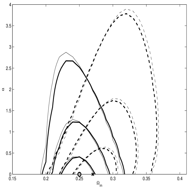
Figure 7: 1, 2, and 3$\sigma$ confidence level contours for the $\phi$CDM model. Solid lines are the joint constraints derived from Percival et al. (2007a) BAO measurements together with WMAP measurement of acoustic horizon angle and galaxy cluster gas mass fraction data ($\circ$ shows the best fit value with an acceptable $\chi^{2}\simeq 58$ for 42 degrees of freedom); dashed lines are the corresponding joint constraints using the Eisenstein et al. (2005) BAO measurement ($\times$ shows the best fit value with an acceptable $\chi^{2}\simeq 52$ for 41 degrees of freedom). Thick lines are derived using the WMAP priors for $h$ and $\Omega_{\rm b}h^{2}$ while thin lines are for the alternate priors. The joint best fit values for the two prior sets overlap. The $\alpha=0$ axis corresponds to spatially-flat $\Lambda$CDM models. The $\Omega_{\rm m}$ and $\alpha$ ranges shown here are smaller than those shown in Fig. 4.

Since the gas mass fraction and BAO peak measurements are statistically independent we define the joint $\chi^{2}$ function by adding together the individual $\chi^{2}$s. The resulting joint constraints are shown in Figs. 5, 6, and 7.

4 Results and discussion

The Eisenstein et al. (2005) BAO peak measurement has been used in conjunction with other data to place constraints on various cosmological models (see, e.g., Alam & Sahni, 2006; Nesseris & Perivolaropulos, 2007; Movahed et al., 2009; Zhang & Wu, 2007; Wright, 2007; Shafieloo, 2007). The more recent Percival et al. (2007a) data has also been used for this purpose (Ishida et al., 2008; Lazkoz et al., 2008).

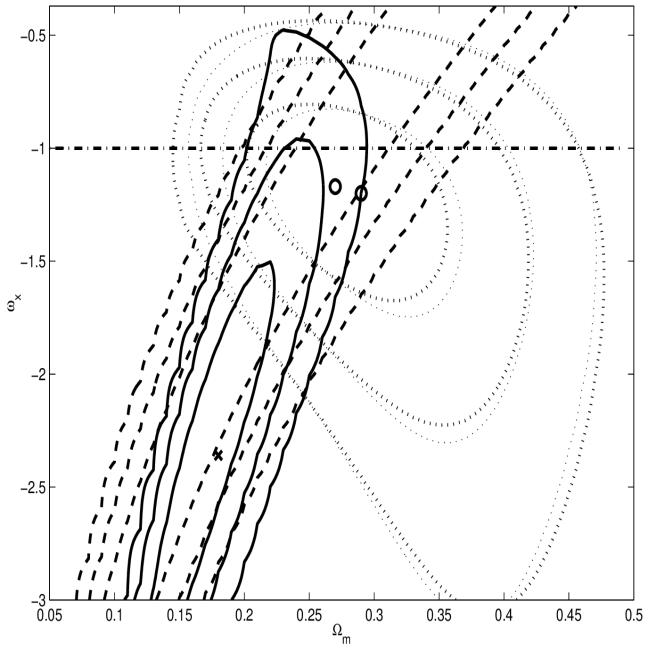
Figure 3: 1, 2, and 3$\sigma$ confidence level contours for the XCDM parametrization. Solid lines are the constraints derived from Percival et al. (2007a) BAO measurements together with WMAP measurement of acoustic horizon angle ($\times$ for the best fit value) and dashed lines are those from the Eisenstein et al. (2005) BAO measurement. The two sets of dotted lines are the constraints derived from galaxy cluster gas mass fraction data (Samushia & Ratra, 2008) ($\circ$ for the best fit value); the thick dotted lines are derived using WMAP priors for $h$ and $\Omega_{\rm b}h^{2}$ while the thin dotted lines are for the alternate priors (see text). The horizontal dot-dashed line corresponds to spatially-flat $\Lambda$CDM models.

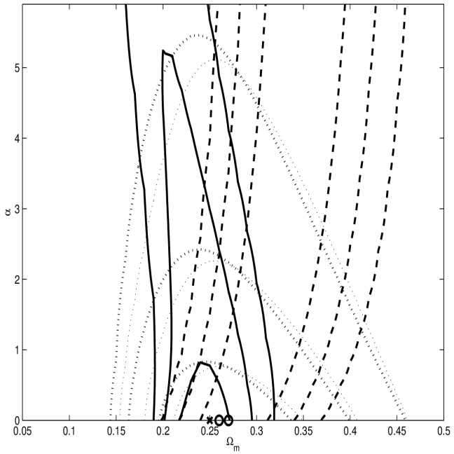
Figure 4: 1, 2, and 3$\sigma$ confidence level contours for the $\phi$CDM model. Solid lines are the constraints derived from Percival et al. (2007a) BAO measurements together with WMAP measurement of acoustic horizon angle ($\circ$ for the best fit value) and dashed lines are those from the Eisenstein et al. (2005) BAO measurement. The two sets of dotted lines are the constraints derived from galaxy cluster gas mass fraction data (Samushia & Ratra, 2008) ($\times$ for the best fit value); the thick dotted lines are derived using WMAP priors for $h$ and $\Omega_{\rm b}h^{2}$ while the thin dotted lines are for the alternate priors (see text). The $\alpha=0$ axis corresponds to spatially-flat $\Lambda$CDM models.

Constraints from BAO peak measurements and galaxy cluster gas mass fraction data are shown in Figs. 2, 3, and 4. The solid line contours in Figs. 2 and 3 show the constraints on $\Lambda$CDM and XCDM derived from the Percival et al. (2007a) BAO data and are comparable to those shown with dashed lines in Fig. 12 in their paper. The dashed contours in Fig. 3 are comparable to those shown in Fig. 11 in Eisenstein et al. (2005). Eisenstein et al. (2005) do not show contours for $\Lambda$CDM (see our Fig. 2) and the BAO contours we show in Fig. 4 have not previously been presented. Figure 2 shows that the Percival et al. (2007a) constraints, which make use of the WMAP measurement of the apparent acoustic horizon angle, constrain the sum of parameters $\Omega_{\Lambda}$ and $\Omega_{\rm m}$ to be very close to one ($\Omega_{\rm k}=1-\Omega_{\rm m}-\Omega_{\Lambda}\approxeq 0$) and favor a close to spatially flat model if dark energy is time independent. The spatial curvature is constrained so well mainly because we use the WMAP measurement of the apparent acoustic peak angle. BAO measurements by themselves can not effectively constrain dark energy parameters very well (see shaded areas in Fig. 12 of Percival et al., 2007a). In spatially-flat models BAO peak measurements put tight constraints on the $\Omega_{\rm m}$ parameter; they do not well constrain the “orthogonal” cosmological parameter $\Omega_{\Lambda}$ and in particular they allow dark energy to vary in time (see Figs. 3 and 4).

The BAO constraints are significantly tighter than the Hubble parameter versus redshift data ones (see, e.g., Samushia et al., 2007) and the strong gravitational lensing ones (see, e.g., Chae et al., 2004). They are, in general, about as constraining as the SNIa results and constrain roughly the same linear combination of cosmological parameters (see, e.g., Wilson et al., 2006). In Figs. 2 and 3 the best fit values from Percival et al. (2007a) measurement and WMAP prior are more then 3$\sigma$ away from the best fit of the cluster gas mass fraction constraints. This is most probably due to unknown systematic errors in one or both of the measurements or an effect of poor statistics and should change when more and better data are available.

The joint BAO peak and cluster gas mass fraction constraints are shown in Figs. 5, 6, and 7. They are fairly restrictive and favor a spatially-flat $\Lambda$CDM model with $\Omega_{\rm m}\sim$ 0.25 and $\alpha<0.5$ on $1\sigma$ confidence level. Since the predictions of $\phi$CDM for a very small value of the $\alpha$ parameter are very close to the predictions of the spatially-flat $\Lambda$CDM model, current observational tests are unable to discriminate between a time-independent cosmological constant and a slowly varying scalar field with $\alpha$ of order 1. All three models considered here give about the same $\chi^{2}\sim 52$ for 41 degrees of freedom and there is no reason to favor one model over another based on Bayesian statistics. The constraints from the joint analysis on all three dark energy models are comparable to the constraints derived from a joint analysis (Wilson et al., 2006) of earlier SNIa data (Riess et al., 2004) and earlier cluster gas mass fraction data (Allen et al., 2004). Constraints on $\alpha$ derived from the joint analysis are stronger than the results quoted in previously published papers (see Table 1) The joint BAO peak and gas mass fraction data constraints on $\Lambda$CDM and XCDM derived here are a little weaker than those derived from BAO peak and more recent SNIa (Astier et al., 2006) data, see Figs. 13 of Percival et al. (2007a). In the joint analysis done here the uncertainties on $h$ and $\Omega_{\rm b}h^{2}$ play a less significant role than they do in the cluster gas mass fraction analysis, i.e., the contours for the two prior sets are closer to each other in Figs. 5, 6, and 7, than in Figs. 2, 3, and 4. The contours in Figs. 5 and 6 are in agreement with tighter joint results from other data sets considered by Wang et al. (2007).

From Fig. 1 it is clear that for large values of $\alpha$ $\phi$CDM and XCDM models predict different cosmological evolution. For small values of $\alpha$, however, if parameters are chosen appropriately, different dark energy models will at low redshifts predict very similar background evolution. Because of that, low redshift distance measurements have to be complemented with high redshift CMB and large scale structure measurements to discriminate between dark energy models. Better quality BAO peak data at a number of redshifts and more gas mass fraction measurements, along with tighter priors on nuisance parameters like the Hubble parameter and the density of baryonic matter, will allow for tighter constraints on dark energy parameters and could soon either detect a time dependence in dark energy or constrain it to a very small value.

Table 1: Constraints on the $\phi$CDM $\alpha$ parameter from different observational tests.

3$\sigma$ constraints on $\alpha$	Observational test(s) used	reference
$\alpha$  not well constrained	SNIa	Podariu & Ratra (2000)
$\alpha$  not well constrained	Radio galaxies	Podariu et al. (2003)
$\alpha$  not well constrained	Gravitational lensing	Chae et al. (2004)
$\alpha<6.5$	Galaxy clusters	Chen & Ratra (2004)
$\alpha<5$	Radio galaxies & SNIa “Gold” data set	Wilson et al. (2006)
$\alpha<5$	Radio galaxies & SNIa	Daly et al. (2007)
$\alpha<4.5$	Galaxy clusters	Samushia & Ratra (2008)
$\alpha<3.5$	Galaxy clusters & BAO	This work

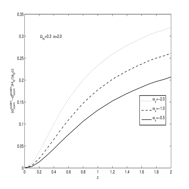
Figure 1: Residuals of comoving distance calculated in the $\phi$CDM model with $\Omega_{\rm m}=0.3$ and $\alpha=2$ and predictions of XCDM parameterization with $\omega_{\rm x}=-0.5$ (solid line), $\omega_{\rm x}=-1.0$ (dashed line), and $\omega_{\rm x}=-2.0$ (dotted line). Comoving distance is normalized to $a_{0}c/H_{0}$.

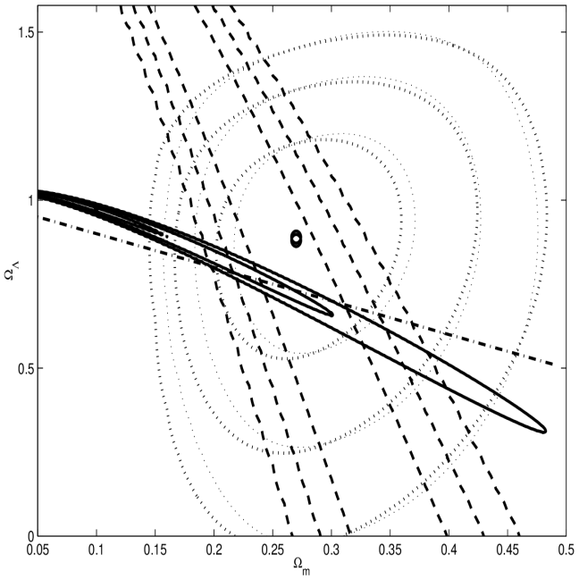
Figure 2: 1, 2, and 3$\sigma$ confidence level contours for the $\Lambda$CDM model. Solid lines are the constraints derived from Percival et al. (2007a) BAO measurements together with WMAP measurement of acoustic horizon angle (the $\times$ for the best fit value near $\Omega_{\rm m}$ is obscured) and dashed lines are those from the Eisenstein et al. (2005) BAO measurement. The two sets of dotted lines are the constraints derived from galaxy cluster gas mass fraction data (Samushia & Ratra, 2008) ($\circ$ for the best fit value); the thick dotted lines are derived using the WMAP priors for $h$ and $\Omega_{\rm b}h^{2}$ while the thin dotted lines are for the alternate priors (see text). The dot-dashed line corresponds to spatially-flat $\Lambda$CDM models.

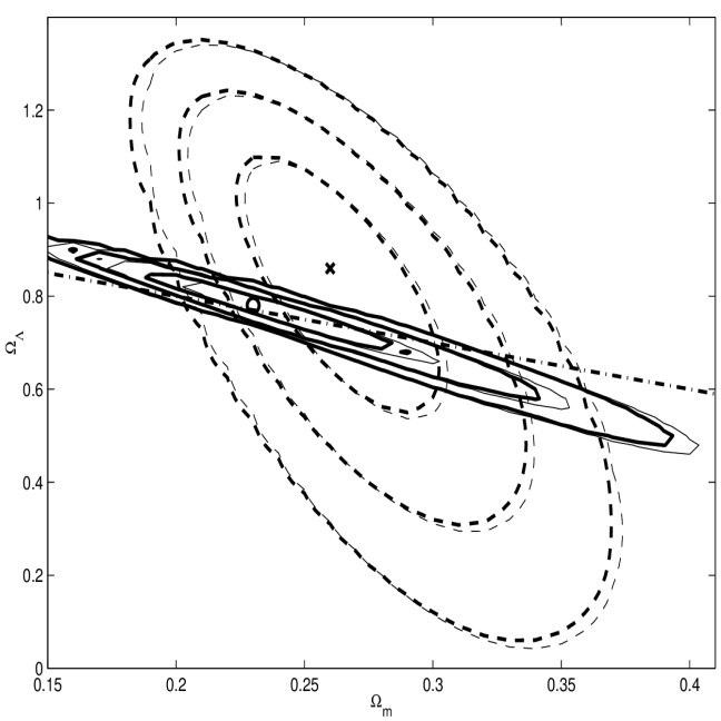
Figure 5: 1, 2, and 3$\sigma$ confidence level contours for the $\Lambda$CDM model. Solid lines are the joint constraints derived from Percival et al. (2007a) BAO measurements together with WMAP measurement of acoustic horizon angle and galaxy cluster gas mass fraction data ($\circ$ shows the best fit value with an acceptable $\chi^{2}\simeq 57$ for 42 degrees of freedom); dashed lines are the corresponding joint constraints using the Eisenstein et al. (2005) BAO measurement ($\times$ shows the best fit value with an acceptable $\chi^{2}\simeq 52$ for 41 degrees of freedom). Thick lines are derived using the WMAP priors for $h$ and $\Omega_{\rm b}h^{2}$ while thin lines are for the alternate priors. The joint best fit values for the two prior sets overlap. The dot-dashed line corresponds to spatially-flat $\Lambda$CDM models. The $\Omega_{\rm m}$ and $\Omega_{\Lambda}$ ranges shown here are smaller than those shown in Fig. 2.

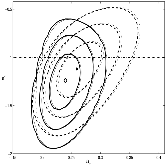
Figure 6: 1, 2, and 3$\sigma$ confidence level contours for the XCDM parametrization. Solid lines are the joint constraints derived from Percival et al. (2007a) BAO measurements together with WMAP measurement of acoustic horizon angle and galaxy cluster gas mass fraction data ($\circ$ shows the best fit value with an acceptable $\chi^{2}\simeq 56.5$ for 42 degrees of freedom); dashed lines are the corresponding joint constraints using the Eisenstein et al. (2005) BAO measurement ($\times$ shows the best fit value with an acceptable $\chi^{2}\simeq 52$ for 41 degrees of freedom). Thick lines are derived using the WMAP priors for $h$ and $\Omega_{\rm b}h^{2}$ while thin lines are for the alternate priors. The joint best fit values for the two prior sets overlap. The horizontal dot-dashed line corresponds to spatially-flat $\Lambda$CDM models. The $\Omega_{\rm m}$ and $\omega_{\rm x}$ ranges shown here are smaller than those shown in Fig. 3.

References

- Alam & Sahni (2006) Alam, U., & Sahni, V. 2006, Phys. Rev. D, 73, 084024
- Allen et al. (2008) Allen, S. W., et al. 2008, MNRAS, 383, 879
- Allen et al. (2004) Allen, S. W., et al. 2004, MNRAS, 353, 457
- Astier et al. (2006) Astier, P., et al. 2006, A&A, 447, 31
- Blake et al. (2007) Blake, C., Collister, A., Bridle, S., & Lahav, O. 2007, MNRAS, 374, 1527
- Blake & Glazebrook (2003) Blake, C., & Glazebrook, K. 2003, ApJ, 594, 665
- Brookfield et al. (2008) Brookfield, A. W., van de Bruck, C., & Hall, L. M. H. 2008, Phys. Rev. D, 77, 043006
- Capozziello et al. (2008) Capozziello, S., Cardone, V. F., & Salzano, V. 2008, Phys. Rev. D, 78, 063504
- Chae et al. (2004) Chae, K.-H., Chen, G., Ratra, B., & Lee, D.-W. 2004, ApJ, 607, L71
- Chen et al. (2003) Chen, G., Gott, J. R., & Ratra, B. 2003, PASP, 115, 1269
- Chen & Ratra (2003a) Chen, G., & Ratra, B. 2003a, ApJ, 582, 586
- Chen & Ratra (2003b) Chen, G., & Ratra, B. 2003b PASP, 115, 1143
- Chen & Ratra (2004) Chen, G., & Ratra, B. 2004, ApJ, 612, L1
- Cole et al. (2005) Cole, S., et al. 2005, MNRAS, 362, 505
- Costa et al. (2008) Costa, F. E. M., Alcaniz, J. S., & Maia, J. M. F. 2008, Phys. Rev. D, 77, 083516
- Daly et al. (2007) Daly., R. A., et al. 2007, ApJ, 691, 1058
- Davis et al. (2007) Davis, T. M., et al. 2007, ApJ, 666, 716
- Dev et al. (2008) Dev, A., Jain, D., & Lohiya, D. 2008, arXiv:0804.3491 [astro-ph]
- Demianski et al. (2008) Demianski, M., Piedipalumbo, E., Rubano, C., & Scudellaro, B. 2008, A&A, 481, 279
- Doran et al. (2007) Doran, M., Robbers, G., & Wetterich, C. 2007, Phys. Rev. D, 75, 023003
- Doré et al. (2007) Doré, O., et al. 2007, arXiv:0712.1599 [astro-ph]
- Eisenstein et al. (2005) Eisenstein, D. J., et al. 2005, ApJ, 633, 560
- Feng et al. (2007) Feng, C., Wang, B., Gong, Y., & Su, R.-K. 2007, J. Cosmology Astropart. Phys, 0709, 005
- Fields & Sarkar (2006) Fields, B. D., & Sarkar, S. 2006, J. Phys. G., 33, 220
- Frieman et al. (2008) Frieman, J. A., Turner, M. S., & Huterer, D. 2008, ARA&A, 46, 385
- Freedman et al. (2000) Freedman, W. L., et al. 2000, ApJ, 553, 42
- Fu et al. (2008) Fu, L., et al. 2008, A&A, 479, 8
- Ganga et al. (1997) Ganga, K., Ratra, B., Gunderson, J. O., & Sugiyama, N. 1997, ApJ, 484, 7
- Gannouji & Polarski (2008) Gannouji, R., & Polarski, D. 2008, J. Cosmology Astropart. Phys, 0805, 018
- Gong et al (2008) Gong, Y., Wu, Q., & Wang, A. 2008, ApJ, 681, 27
- Gott et al. (2001) Gott, J. R., Vogeley, M. S., Podariu, S., & Ratra, B. 2001, ApJ, 549, 1
- Grande et al. (2007) Grande, J., Opher, R., Pelinson, A., & Solà, J. 2007, J. Cosmology Astropart. Phys, 0712, 007
- He & Wang (2008) He, J.-H., & Wang, B. 2008, J. Cosmology Astropart. Phys, 06, 010
- Hu & Haiman (2003) Hu, W., & Haiman, Z. 2003, Phys. Rev. D, 68, 063004
- Hütsi (2006) Hütsi, G. 2006, A&A, 449, 891
- Ichikawa & Takahashi (2008) Ichikawa, K., & Takahashi, T. 2008, J. Cosmology Astropart. Phys, 0804, 027
- Ichiki & Keum (2008) Ichiki, K., & Keum, Y.-Y. 2008, JHEP, 0806, 058
- Ishida et al. (2008) Ishida, É. E. O., Reis, R. R. R., Toribo, A. V., & Waga, I. 2008, Astropart. Phys., 28, 547
- Kirkman et al. (2003) Kirkman, D., et al. 2003, ApJS, 149, 1
- Kowalski et al. (2008) Kokwalski, M., et al. 2008, ApJ, 686, 749
- Kurek & Szydłowsky (2008) Kurek, A., & Szydłowski, M. 2008, ApJ, 675, 1
- La Vacca & Colombo (2008) La Vacca, G., & Colombo, L. P. L. 2008, J. Cosmology Astropart. Phys, 0804, 007
- Lazkoz & Majerotto (2007) Lazkoz, R., & Majerotto, E. 2007, J. Cosmology Astropart. Phys, 0707, 015
- Lazkoz et al. (2008) Lazkoz, R., Nesseris, S., & Perivolaropulos, L. 2008, J. Cosmology Astropart. Phys, 07, 012
- Lee & Ng (2007) Lee., S., & Ng, K.-W. 2007, Phys. Rev. D, 76, 043518
- Lima et al. (2007) Lima, J. A. S., Jesus, J. F., & Cunha, J. V. 2007, ApJ, 690, L85
- Lin et al. (2008) Lin, H., Zhang, T.-J., & Yuan, Q. 2008, arXiv:0804.3135 [astro-ph]
- Linder (2003) Linder, E. V., 2003, Phys. Rev. D, 68, 083504
- Linder (2008) Linder, E. V. 2008, Rept. Prog. Phys., 71, 056901
- Liu et al. (2008) Liu, D.-J., Li, X.-Z., Hao, J., & Jin, X.-H. 2008, MNRAS, 388, 275
- Mainini & Bonometto (2007) Mainini, R., & Bonometto, S. 2007, J. Cosmology Astropart. Phys, 0709, 017
- Martin (2008) Martin, J. 2008, Mod. Phys. Lett. A, 23, 1252
- Mathews et al. (2008) Mathews, G. J., Lan, N. Q., & Kolda, C. 2008, Phys. Rev. D, 78, 043525
- Mignone & Bartelmann (2008) Mignone, C., & Bartelmann, M. 2008, A&A, 481, 295
- Movahed et al. (2009) Movahed, M. S., Farhang, M., & Rahvar, S. 2009, Int. J. Theor. Phys., 48, 1203
- Nesseris & Perivolaropulos (2007) Nesseris, S., & Perivolaropulos, L. 2007, J. Cosmology Astropart. Phys, 0701, 018
- Neupane & Scherer (2008) Neupane, I. P., & Scherer, C. 2008, J. Cosmology Astropart. Phys, 0805, 009
- Oguri et al. (2008) Oguri, M., et al. 2008, AJ, 135, 512
- Olivares et al. (2008) Olivares, G., Atrio-Barandela, F., & Pavón, Phys. Rev. D, 77, 3520
- Padmanabhan et al. (2007) Padmanabhan, N., et al. 2007, MNRAS, 378, 852
- Page et al. (2003) Page, L., et al. 2003, ApJS, 148, 233
- Peebles (1984) Peebles, P. J. E. 1984, ApJ, 284, 439
- Peebles (1993) Peebles, P. J. E. 1993, Principles of Physical Cosmology (Princeton: Princeton University Press)
- Peebles & Ratra (1988) Peebles, P. J. E., & Ratra, B. 1988, ApJ, 325, L17
- Peebles & Ratra (2003) Peebles, P. J. E., & Ratra, B. 2003, Rev. Mod. Phys., 75, 559
- Peebles & Yu (1970) Peebles, P. J. E., & Yu, J. T. 1970, ApJ, 162, 815
- Pen (1997) Pen, U.-L. 1997, New A, 2, 309
- Percival et al. (2007b) Percival, W. J., et al. 2007b, ApJ, 657, 51
- Percival et al. (2007a) Percival, W. J., et al. 2007a, MNRAS, 381, 1053
- Perlmutter et al. (1999) Perlmutter, S., et al. 1999, ApJ, 517, 565
- Podariu et al. (2003) Podariu, S., Daly, R. A., Mory, M., & Ratra, B. 2003 ApJ, 584, 577
- Podariu et al. (2001a) Podariu, S., Nugent, P., & Ratra, B. 2001a, ApJ, 553, 39
- Podariu & Ratra (2000) Podariu, S., & Ratra, B. 2000, ApJ, 532, 109
- Podariu et al. (2001b) Podariu, S., Souradeep, T., Gott, J. R., Ratra, B., & Vogeley, M. S. 2001b, ApJ, 559, 9
- Rapetti et al. (2005) Rapetti, D., Allen, S. W., & Weller, J. 2005, MNRAS, 360, 555
- Ratra (1991) Ratra, B. 1991, Phys. Rev. D, 43, 3802
- Ratra & Peebles (1988) Ratra, B., & Peebles, P. J. E. 1988, Phys. Rev. D, 37, 3406
- Ratra & Vogeley (2008) Ratra, B., & Vogeley, M. S. 2008, PASP, 120, 235
- Riess et al. (1998) Riess, A. G., et al. 1998, AJ, 116, 1009
- Riess et al. (2004) Riess, A. G., et al. 2004, ApJ, 607, 665
- Samushia et al. (2007) Samushia, L., Chen, G., & Ratra, B. 2007, arXiv:0706.1963 [astro-ph]
- Samushia & Ratra (2006) Samushia, L., & Ratra, B. 2006, ApJ, 650, L5
- Samushia & Ratra (2008) Samushia, L., & Ratra, B. 2008, ApJ, 680, L1
- Santos & Lima (2008) Santos, R. C., & Lima, J. A. S. 2008, Phys. Rev. D, 77, 083505
- Sapone & Amendola (2007) Sapone, D., & Amendola, L. 2007, arXiv:0709.2792 [astro-ph]
- Sasaki (1996) Sasaki, S. 1996, PASJ, 48, 119
- Sen (2008) Sen, A. A. 2008, Phys. Rev. D, 77, 043508
- Seo & Eisenstein (2003) Seo, H.-J., & Eisenstein, D. J. 2003, ApJ, 598, 720
- Shafieloo (2007) Shafieloo, A. 2007, MNRAS, 380, 1573
- Spergel et al. (2007) Spergel, D. N., et al. 2007, ApJS, 170, 377
- Sunyaev & Zel’dovich (1970) Sunyaev, R. A., & Zel’dovich, Ya. B. 1970, Ap&SS, 7, 3
- Szydłowski et al. (2008) Szydłowski, M., Hrycyna, O., & Kurek, A. 2008, Phys. Rev. D, 77, 027302
- Takada & Bridle (2007) Takada, M., & Bridle, S. 2008, New J. Phys., 9, 46
- Tsujikawa et al. (2008) Tsujikawa, S., Uddin, K., & Tavakol, R. 2008, Phys. Rev. D, 77, 043007
- Usmani et al. (2008) Usmani, A. A., et al. 2008, MNRAS, 386, 92
- Virey et al. (2008) Virey, J. M., et al. 2008, J. Cosmology Astropart. Phys, 12, 008
- Wang et al. (2007) Wang, F. Y., Dai, Z. G., and Zhu, Z.-H. 2007, ApJ, 667, 1
- Wang (2007) Wang, Y. 2007, arXiv:0712.0041 [astro-ph]
- Wang (2008) Wang, Y. 2008, J. Cosmology Astropart. Phys, 05, 021
- Wang & Mukherjee (2007) Wang, Y., & Mukherjee, P. 2007, Phys. Rev. D, 76, 103533
- Wei (2008) Wei, H. 2008, Phys. Lett. B, 664, 1
- Wei & Zhang (2008) Wei, H., & Zhang, S. N. 2008, Phys. Rev. D, 76, 063003
- Wilson et al. (2006) Wilson. K. M., Chen. G., & Ratra. B. 2006, Mod. Phys. Lett. A, 21, 2197
- Wright (2007) Wright, E. L. 2007, ApJ, 664, 633
- Wu & Yu (2008) Wu, P., & Yu, H. 2008, J. Cosmology Astropart. Phys, 0802, 019
- Wu et al. (2008) Wu, Q., Gong, Y., Wang, A., & Alcaniz, J. S. 2008, Phys. Lett. B, 659, 34
- Xia et al. (2007) Xia, J.-Q., Li, H., Zhao, G.-B., & Zhang, X. 2008, Int. J. Mod. Phys. D, 17, 2025
- Zhang et al. (2007) Zhang, Q.-J., Cheng, L.-M., & Wu, Y.-L. 2007,
- Zhang & Wu (2007) Zhang, X., & Wu, F.-Q. 2007, Phys. Rev. D, 76, 023502
- Zhu & Sereno (2008) Zhu, Z.-H., & Sereno, M. 2008, A&A, 487, 831