CP Violation in the SUSY Seesaw:
Leptogenesis and Low Energy

Abstract:

We suppose that the baryon asymmetry is produced by thermal leptogenesis (with flavour effects), at temperatures $\sim 10^{9}-10^{10}$ GeV, in the supersymmetric seesaw with universal and real soft terms. The parameter space is restricted by assuming that $\ell_{\alpha}\to\ell_{\beta}\gamma$ processes will be seen in upcoming experiments. We study the sensitivity of the baryon asymmetry to the phases of the lepton mixing matrix, and find that leptogenesis can work for any value of the phases. We also estimate the contribution to the electric dipole moment of the electron, arising from the seesaw, and find that it is (just) beyond the sensitivity of next generation experiments ($\mathrel{\vbox{\hbox{$<$}\nointerlineskip\hbox{$\sim$}}}10^{-29}e$ cm). The fourteen dimensional parameter space is efficiently explored with a Monte Carlo Markov Chain, which concentrates on the regions of interest.

1 Introduction

Neutrino masses are evidence for beyond the Standard Model (SM) physics. A simple extension of the standard model that accounts for neutrino masses is the seesaw mechanism [1], where heavy majorana right-handed neutrinos are added to the SM. Moreover, the seesaw scenario provides a very attractive framework to explain the baryon asymmetry of the universe (BAU) through the leptogenesis [2] mechanism, without inducing proton decay.

CP violation is a necessary ingredient to explain the BAU and, if this asymmetry is produced via leptogenesis, the required CP violation is encoded in the CP violating phases of the lepton sector. Three of them are the well known Dirac and Majorana phases of the PMNS mixing matrix, that are in principle measurable. Any observation of CP violation in the lepton sector, for instance CP violation in neutrino oscillations due to the PMNS phase $\delta$, would then support leptogenesis by demonstrating that CP is not a symmetry of leptons. However, even in this very promising case, the question of whether the BAU is produced via leptogenesis is far from being answered, because it is not possible to reconstruct the high-energy CP odd observables from the low-energy ones [3] without assuming very constraining frameworks for the unmeasurable quantities. Therefore, the intent of this work is to clarify the relation between the CP violation accessible to low-energy experiments, and the CP violation necessary for leptogenesis, in a phenomenological bottom-up perspective, with minimal assumptions about the high scale theory. We just assume that the neutrino Yukawa couplings are hierarchical, which is the most natural assumption given the observed values of the charged lepton and quark Yukawas. Neutrino oscillation data then lead to hierarchical singlet masses.

In this paper, we aim to answer the phenomenological question of whether the BAU can be sensitive to low-energy phases, in the supersymmetric seesaw. We suppose the observed BAU is generated via thermal leptogenesis, and enquire whether this restricts the range of the phases. A similar issue was investigated by Branco et.al [4], where it was shown that for any value of the measurable CP violating phases, a large enough BAU can be produced. This statement has been recently confirmed in a study [5] that includes flavour effects [6], in the Standard Model seesaw framework. In the present analysis, we want to address the question considering flavoured leptogenesis in a supersymmetric scenario, that has the interesting feature to potentially add new observables in the lepton sector, through the enhancement of flavour and CP violating processes (See eg [7] for a review and references on leptonic flavour and CP violation, induced by supersymmetry.).

The question we address, and the answer we find, differ from some other analyses [8, 9, 10, 11]. As written above, we aim to make few untestable assumptions, and to ask a precise phenomenological question: “Is the baryon asymmetry sensitive to PMNS phases?”. We find the answer to be no. That is, there is “no correlation” between the BAU and PMNS phases, when all the unmeasurables in our scenario are allowed to vary over their whole range. To the best of our understanding, Refs. [8, 9, 10, 11] find a correlation between the BAU and the PMNS phases because they set unmeasurables (such as phases of the “right-handed” neutrinos) to fixed values.

We define “finding a correlation between $Y_{B}$ and $x$” to mean “$Y_{B}$ is sensitive to $x$”. To show that the baryon asymmetry $Y_{B}$ is insensitive to (or uncorrelated with) a parameter $x$, we must only show that, for any value of $x$, we can find a large enough $Y_{B}$. It would be numerically more challenging to show a correlation, because the point distribution in scatter plots may reflect the priors on the scanned parameters (see sections 6.4 and 7.2). Our definition of correlation differs from that used by [8, 9, 11], and also in [19] (who extract correlations from scatter plots). We use our narrow definition because it is parametrisation independent.

Since leptogenesis occurs at a very high-energy scale, a supersymmetric scenario is desirable in order to stabilize the hierarchy between the leptogenesis scale and the electroweak one. However, if supersymmetry exists at all, it must be broken and, in principle, the soft supersymmetry breaking Lagrangian can contain off-diagonal (in flavour space) soft terms, that would enhance lepton flavour violating (LFV) processes. These are strongly constrained by current experiments; this is the so-called supersymmetric flavour problem. In order to avoid it, we focus on the most conservative minimal Supergravity (MSUGRA) scenario with real boundary conditions, where the dynamics responsible for supersymmetry breaking are flavour blind and all the lepton flavour and CP violation is controlled by the neutrino Yukawa couplings. Supersymmetric expectations for LFV [12, 13, 14] and possible relations to leptogenesis [7, 11, 15, 16, 17, 18] and EDMs [19, 20] have been studied by many people.

We perform a scan over the seesaw parameters, looking for those points that give a large enough BAU, and where $\mu\to e\gamma$ and one of $\tau\to\ell\gamma$ would be seen in upcoming experiments. Our analysis is more restrictive than [19], in that we require these branching ratios to be “large”. The aim is to verify if such experimental inputs imply a preferred range of values for the low-energy PMNS phases. We also estimate the contribution to the CP violating electron electric dipole moment. A detailed analysis of the MSUGRA scenario would require a scan also over the supersymmetric parameters, which is beyond the scope of our analysis.

Due to the large number of unknown parameters, instead of doing a usual grid scan in the seesaw parameter space we construct a Markov Chain using a Monte Carlo simulation (MCMC — see e.g. [21, 22]). This technique allows to efficiently explore a high-dimension parameter space, and we apply it for the first time to the supersymmetric seesaw model . Our work is thus pioneering in the exhaustive scanning of the seesaw parameters, which would be otherwise prohibitive without the MCMC technique.

The paper is organized as follows. In section 2 we introduce the supersymmetric seesaw in the MSUGRA scenario and we review the low-energy interactions induced in the supersymmetric seesaw model. Section 3 is devoted to thermal leptogenesis with flavour effects, and section 4 describes our bottom-up reconstruction procedure. Section 5 gives analytic estimates, that complement our numerical analysis, using the MCMC technique, which is presented in section 6. We discuss our results in section 7 and conclude in section 8.

2 Notation and review

We consider the superpotential for the leptonic sector in a supersymmetric seesaw model [1] with three hierarchical right-handed neutrinos ($M_{1}<M_{2}<M_{3}$):

$$W_{lep}=(L_{L}H_{d}){Y_{e}}E^{c}+({L_{L}}H_{u}){\lambda}N^{c}+N^{c}\frac{M}{2}N^{c}.$$ (1)

In this expression, $\lambda,Y_{e}$ and $M$ are $3\times 3$ matrices, and flavour indices are suppressed. The $L_{L}$ are the supermultiplets containing left-handed lepton fields, $E$ are those containing the right-handed charged leptons, while $N$ are the supermultiplets of the right-handed singlets. The Majorana mass scale can be taken large $10^{9}$ GeV $\mathrel{\vbox{\hbox{$<$}\nointerlineskip\hbox{$\sim$}}}M_{i}\mathrel{\vbox{\hbox{$<$}\nointerlineskip\hbox{$\sim$}}}10^{15}$ GeV, since the corresponding operator is a singlet under the SM gauge group.

Without loss of generality one can work in the basis where $Y_{e}$ and $M$ are diagonal, so that the superpotential gives the following Lagrangian for leptons:

$${\cal L}=Y_{e_{\alpha}}(\overline{\ell}_{L}^{\alpha}H^{*}_{d})e_{R}^{\alpha}+(\overline{\ell}_{L}^{\alpha}H^{*}_{u}){\bf\lambda^{*}}_{\alpha i}N_{i}+\frac{{M}^{i}}{2}\overline{N^{c}}_{i}N_{i}+...+h.c.$$ (2)

where the parentheses indicate SU(2) contractions and the flavour indices are written explicitly. Since supersymmetry is broken, to this Lagrangian we must add the soft SUSY breaking terms :

$$\mathcal{L}_{SSB}=\tilde{m}_{0}^{2}\sum_{f}\tilde{f}^{\dagger}\tilde{f}+\left\{\frac{BM^{i}}{2}\tilde{N}_{i}^{c}\tilde{N}_{i}^{c}+a_{0}(y_{e_{\alpha}}{\tilde{\ell}_{L}}^{\alpha}\cdot H_{d}\tilde{e}_{\alpha}^{c}+\lambda_{\alpha i}\tilde{\ell}^{\alpha}_{L}\cdot H_{u}\tilde{N}_{i}^{c})+h.c.\right\}$$ (3)

where $\tilde{f}$ collectively represents sfermions. This soft part is written at some high scale $M_{X}$ where, in MSUGRA, the soft masses are universal and the trilinear couplings are proportional to the corresponding Yukawas. MSUGRA is then characterized by four parameters: the scalar ($m_{0}$) and gaugino ($m_{1/2}$) masses, shared by all of them at the GUT scale; the trilinear coupling involving scalars, $a_{0}$, at the GUT scale; and finally the Higgs vev ratio, $\tan\beta$.

In the chosen basis, the neutrino Yukawa matrix is in general not diagonal and complex, and can be written as:

$$\lambda=V_{L}^{\dagger}D_{\lambda}V_{R}$$ (4)

where $D_{\lambda}$ is diagonal and real. Note that in this basis the neutrino Yukawa matrix is the only source of flavour violation in the lepton sector, through the unitary matrices $V_{L}$ and $V_{R}$ that act respectively on the lepton doublet space and on the right-handed neutrino space. These matrices contribute also to CP violation, through six CP violating phases. In general, other sources of CP violation appear in the complex neutrino B-term, in the scalar mass $\tilde{m}_{0}$ and in the trilinear coupling $a_{0}$.

At energies well below the right-handed neutrino mass scale, the effective light neutrino majorana mass matrix can be written:

$$[m_{\nu}]=\lambda M^{-1}\lambda^{T}v_{u}^{2}=UD_{\nu}U^{T}.$$ (5)

The first equality shows that the smallness of light neutrino masses is naturally explained once the right-handed neutrino mass is set at very high energy, $\sim 10^{14}$ GeV (in this expression $v_{u}=\langle H_{u}\rangle$). In the second equality, $D_{\nu}$ is a diagonal matrix with real positive eigenvalues and $U$ is the $PMNS$ matrix containing the three low-energy CP violating phases, the Dirac phase $\delta$ and two Majorana phases $\alpha$, $\beta$. Those phases are, in general, a combination of the 6 phases appearing in the complete theory. We use the standard parametrisation:

$$U=\left(\begin{array}[]{ccc}e^{i\alpha}~{}c_{13}c_{12}&e^{i\beta}~{}s_{12}c_{13}&s_{13}~{}e^{-i\delta}\\ e^{i\alpha}~{}(-s_{12}c_{23}-s_{23}s_{13}c_{12}~{}e^{i\delta})&e^{i\beta}~{}(c_{23}c_{12}-s_{23}s_{13}s_{12}~{}e^{i\delta})&s_{23}c_{13}\\ e^{i\alpha}~{}(s_{23}s_{12}-s_{13}c_{23}c_{12}~{}e^{i\delta})&e^{i\beta}~{}(-s_{23}c_{12}-s_{13}s_{12}c_{23}~{}e^{i\delta})&c_{23}c_{13}\end{array}\right).$$ (6)

If we combine the equations (4) and (5), we can write:

$$D_{\nu}=U^{\dagger}V_{L}^{\dagger}D_{\lambda}V_{R}D_{M}^{-1}V_{R}^{T}D_{\lambda}V_{L}^{*}U^{*}v_{u}^{2}\equiv W^{\dagger}D_{\lambda}V_{R}D_{M}^{-1}V_{R}^{T}D_{\lambda}W^{*}v_{u}^{2},$$ (7)

with $V_{R}$ diagonalizing the inverted right-handed neutrino mass matrix. This relation shows that non-zero angles and phases in the unmeasurable right-handed neutrino mixing matrix $V_{R}$ imply non-zero angles and phases in $W=V_{L}U$, which being in the doublet sector, is potentially more accessible. We will use this relation to reconstruct the right-handed sector from low energy physics in sec. 4.

2.1 Low-energy footprints: LFV and EDMs in MSUGRA

Present bounds on LFV processes, shown in table 1, restrict the size of flavour off-diagonal soft terms. This suggests universal soft terms at some high scale $M_{X}$, see Eq. (3), like in the MSUGRA scenario. There are also stringent experimental bounds, as we can see in Table (2), on the CP violating electric dipole moments, which point towards very small CP phases. To address this “SUSY CP problem” , we suppose that all the soft breaking terms (namely $a_{0}$, $m_{0}$ and right-handed sneutrino B-term), as well as the $\mu$ term, are real. Even under this extremely conservative assumptions, it is well known that because of RGE running from high to low energy scales, the seesaw Yukawa couplings potentially induce lepton flavour and CP violating contributions to the soft terms [12, 13, 14].

	Present bounds	Future sensitivity
BR($\mu\rightarrow e\gamma$)	$<1.2\times 10^{-11}$	$10^{-13}$ (MEG)[25]
BR($\tau\rightarrow\mu\gamma$)	$<6.8\times 10^{-8}$	$10^{-9}$ (Belle)[26]
BR($\tau\rightarrow e\gamma$)	$<1.1\times 10^{-7}$
BR($\mu\rightarrow e\bar{\nu}_{e}\nu_{\mu}$)	$\sim 100\%$
BR($\tau\rightarrow\mu\bar{\nu}_{\mu}\nu_{\tau}$)	$17.36\pm 0.05\%$
BR($\tau\rightarrow e\bar{\nu}_{e}\nu_{\mu}$)	$17.84\pm 0.05\%$

Table 1: Present and predicted bounds on lepton flavour violating processes, and measured branching ratios for $\ell_{\alpha}\rightarrow\ell_{\beta}\nu_{\alpha}\bar{\nu}_{\beta}$ decays.

Present bounds (e cm)	Future sensitivity (e cm)
$d_{e}<1.6\times 10^{-27}$	$10^{-29}$ (Yale group)[27]
$d_{\mu}<2.8\times 10^{-19}$	$10^{-24}$ (Muon EDM Collaboration) [28]
$(-2.2<d_{\tau}<4.5)\times 10^{-17}$

Table 2: Present and anticipated bounds on electric dipole moments. See [7] for a discussion of future experiments.

We focus on these neutrino Yukawa coupling contributions to LFV and EDMs, assuming MSUGRA with real boundary conditions at $M_{X}$. Additional contributions, arising with less restrictive boundary conditions, are unlikely to cancel the ones we discuss, so the upper bounds that will be set if, for instance, no electron EDM is measured by the Yale group, will equally apply. Conversely, if an electron EDM is measured above the range that we predict, it will prove the existence of a source of CP violation other than the neutrino Yukawa phases.

We are interested in analytic estimates for LFV rates and electric dipole moments. For this, we need the flavour-changing and CP violating contributions to the soft masses, that arise from the neutrino Yukawa. Following [29], we take the one-loop corrections to the flavour off-diagonal doublet slepton masses $\widetilde{m}^{2}_{L\alpha\beta}\to\widetilde{m}^{2}_{L\alpha\beta}+\Delta\widetilde{m}^{2}_{L\alpha\beta}$ and to the trilinear coupling $a_{0}\lambda\to a_{0}\lambda(1+\Delta a_{0})$ to be:

$$\Delta\widetilde{m}^{2}_{L\alpha\beta} = -\frac{1}{16\pi^{2}}(3m_{0}^{2}+a_{0}^{2})[C^{(1)}]_{\alpha\beta}-\frac{1}{16\pi^{2}}(m_{0}^{2}+a_{0}^{2}+2a_{0}B)[H]_{\alpha\beta}~{},$$ (8)

$$\Delta(a_{0})_{\alpha\beta} = -\frac{1}{16\pi^{2}}[C^{(1)}]_{\alpha\beta}-\frac{1}{16\pi^{2}}[H]_{\alpha\beta}~{},$$ (9)

for $\alpha\neq\beta$ where the matrices $H$ and $C^{(n)}$ are given by:

$$H\equiv\lambda\lambda^{\dagger}=V_{L}^{\dagger}D_{\lambda}^{2}V_{L}~{},$$ (10)

$$C^{(n)}\equiv\lambda\log^{n}\left(\frac{MM^{\dagger}}{M_{X}^{2}}\right)\lambda^{\dagger}=V_{L}^{\dagger}D_{\lambda}V_{R}\log^{n}\left(\frac{MM^{\dagger}}{M_{X}^{2}}\right)V_{R}^{\dagger}D_{\lambda}V_{L}~{}.$$ (11)

$C^{(1)}$ is the leading log contribution, and terms $\propto H$ arise in the finite part (they could be relevant for EDMs). The one loop corrections to the right handed charged slepton mass matrix, $\widetilde{m}^{2}_{R\alpha\beta}$ only contain the charged lepton Yukawa couplings and therefore cannot generate off-diagonal entries. These are generated at two loops and, as we will see later, they can be relevant for the lepton EDMs.

At one loop, sparticles generate the dipole operator (where $e$ without subscript is the electro-magnetic coupling constant):

$$eX_{\alpha\beta}\overline{e_{L}}^{\alpha}\sigma^{\mu\nu}e_{R}^{\beta}F_{\mu\nu}+h.c.$$ (12)

which leads to LFV decays ($\ell_{\alpha}\rightarrow\ell_{\beta}\gamma$), and induces the flavour diagonal anomalous magnetic and electric dipole moments of charged leptons [7]. For $\alpha=\beta$, the anomalous magnetic moment is $a_{\alpha}=4m_{e_{\alpha}}{\rm Re}\{X_{\alpha\alpha}\}$ and the electric dipole moment is $2{\rm Im}\{X_{\alpha\alpha}\}$.

In the mass insertion approximation the observable LFV rates are proportional to $|\widetilde{m}^{2}_{L\alpha\beta}|^{2}\propto|C^{(1)}_{\alpha\beta}|^{2}$ and the corresponding branching ratios are of order [13]:

$$\frac{BR(\ell_{\alpha}\to\ell_{\beta}~{}\gamma)}{BR(\ell_{\alpha}\rightarrow\ell_{\beta}\nu_{\alpha}\bar{\nu}_{\beta})} \sim \frac{\alpha^{3}}{G_{F}^{2}}\frac{\tan^{2}\beta}{m_{SUSY}^{8}}|\widetilde{m}^{2}_{\alpha\beta}|^{2}$$

$$\sim \frac{\alpha^{3}}{G_{F}^{2}}\frac{\tan^{2}\beta}{m_{SUSY}^{8}}\frac{(3m_{0}^{2}+a_{0}^{2})^{2}}{(4\pi)^{4}}|[C]_{\alpha\beta}|^{2},$$

where $G_{F}$ is the Fermi constant, $\tan\beta=v_{u}/v_{d}$, and $m_{SUSY}$ is a generic SUSY mass, which substitutes for the mixing angles and the function of the loop particle masses.

An estimate of $m_{SUSY}$ can be obtained from the data on the anomalous magnetic moment of the muon, as suggested in [30]. A $3.3$ or $3.4\sigma$ deviation from the Standard Model prediction is observed in the anomalous magnetic moment of the muon (in Table (3) is given the experimental value of $a_{\mu}$ and the deviation from the SM prediction [31, 32]). We assume it is due to new physics that can also contribute to flavour violation and EDMs. In the MSUGRA seesaw scenario that we are considering, the main contribution to $a_{\mu}$ comes from 1-loop diagrams with neutralino or chargino exchange and is given by [33]:

$$\delta a^{SUSY}_{\mu}\simeq\frac{\alpha m^{2}_{\mu}}{8\pi\sin^{2}\theta_{weak}}\frac{\tan\beta}{m^{2}_{SUSY}}.$$ (14)

$a^{EXP}_{\mu}$	$(116~{}592~{}080\pm 63)\times 10^{-11}$ in BNK-E821
	$(276\pm 81)\times 10^{-11}$ [31]
$\delta a_{\mu}=a_{\mu}^{EXP}-a_{\mu}^{SM}$	$(275\pm 84)\times 10^{-11}$ [34]
	$(295\pm 88)\times 10^{-11}$ [32]

Table 3: Experimental value and deviation from the SM predictions of the muon anomalous magnetic moment. The errors of $\delta a_{\mu}$ are the combination in quadrature of the experimental and theoretical ones.

Within this approximation, the observed deviation in the muon anomalous magnetic moment only fixes the ratio $\tan\beta/m_{SUSY}^{2}\sim 5~{}10^{-5}~{}GeV^{-2}$, so our SUSY masses scale with $\tan\beta$ as $m_{SUSY}^{2}=\frac{\tan\beta}{2}(200$ GeV)².

Assuming [30] that the main contribution to the LFV branching ratio is given by analogous diagrams involving chargino and neutralino exchange, gives, from equations (2.1) and (14) with $m_{0}\simeq a_{0}\simeq m_{SUSY}$:

$$\frac{BR(\ell_{\alpha}\to\ell_{\beta}~{}\gamma)}{BR(\ell_{\alpha}\rightarrow\ell_{\beta}\nu_{\alpha}\bar{\nu}_{\beta})}\sim 10^{-8}|C_{\alpha\beta}|^{2}\left(\frac{\delta a_{\mu}}{10^{-9}}\right)^{2}.$$ (15)

Since we aim to explore seesaw parameter space, we set the MSUGRA parameters $m_{0}\simeq a_{0}\simeq m_{SUSY}$.

In our analysis, we aim for values of $|C_{\alpha\beta}|^{2}$ that will give $\mu\to e\gamma$ and either of $\tau\to\ell\gamma$ in the next round of experiments. We require only one of the $\tau$ decays, because the other must be small to suppress $\mu\to e\gamma$ (recall that we assume the neutrino Yukawas are hierarchical).

The neutrino Yukawa corrections to the soft terms can also enhance the predictions of the CP violating electric dipole moments. In our discussion we can neglect muon and tau EDMs, because the experimental sensitivity on $d_{\mu}$ is currently eight orders of magnitude weaker than on $d_{e}$ and we expect $d_{\mu}/d_{e}\sim m_{\mu}/m_{e}$.

There are two potentially important contributions to the charged lepton EDMs induced by the neutrino Yukawa couplings. As discussed in [35, 29], the first non-zero contribution to the complex, flavour diagonal EDMs arises at two-loop order. The matrices $\Delta a_{0}$ and $\Delta\widetilde{m}_{L}^{2}$ in Eq.(8) are the available building blocks to make an EDM, which turns out to be proportional to the commutator $[H,C]$. This is the dominant contribution at low $\tan\beta$.

We follow [29] to estimate:

$$d_{e}\sim\frac{4\alpha}{(4\pi)^{5}}\frac{m_{e}^{2}}{m_{SUSY}^{2}}{\rm Im}[H~{}C]_{ee}(1.9~{}10^{-11}~{}\textrm{e cm})\sim 10^{-29}~{}\left(\frac{2}{\tan\beta}\right){\rm Im}[H~{}C]~{}\textrm{e cm}~{},$$ (16)

where we have used $[H,C]/i=2{\rm Im}[H~{}C]$, and the $2/\tan\beta$ arises because we extracted $m_{SUSY}^{2}$ from the $\delta a_{\mu}$.

In the large $\tan\beta$ region, it has been shown [36] that a different contribution to the EDMs can be the dominant one. This new contribution arises at three loops, and it involves the two loop correction to the right handed charged slepton mass matrix $\Delta\widetilde{m}_{E}^{2}$. It is proportional to the CP violating quantity:

$$D_{\alpha}={\rm Im}\left[((\Delta\widetilde{m}_{E}^{2})^{T}m\Delta\widetilde{m}_{L}^{2}\right]_{\alpha\alpha}$$ (17)

where $m$ is the (diagonal) charged lepton mass matrix. Despite being a higher loop order, it is typically dominant for $\tan\beta\mathrel{\vbox{\hbox{$>$}\nointerlineskip\hbox{$\sim$}}}10$. The two loop expression for $\Delta\widetilde{m}_{E}^{2}$ can be found in [29]. We approximate this contribution as:

$$d_{e} \simeq \frac{-e}{2}\frac{8\alpha}{(4\pi)^{7}}\frac{10m_{e}\tan\beta}{m_{SUSY}^{2}}\frac{{\rm Im}[\lambda_{ek}^{*}\lambda_{\alpha k}m_{\ell_{\alpha}}^{2}\lambda_{\alpha m}^{*}\lambda_{em}]}{v^{2}\cos^{2}\beta}F(M_{k}^{2}),$$ (18)

where

$$F(M_{k}^{2})=\left(\log\frac{M_{X}^{2}}{M_{N}^{2}}\log\frac{M_{X}^{2}}{M_{k}^{2}}\log\frac{M_{N}^{2}}{M_{k}^{2}}+\log^{2}\frac{M_{N}^{2}}{M_{k}^{2}}\log\frac{M_{N}^{2}}{M_{m}^{2}}\right),$$ (19)

and $M_{X}=3\times 10^{16}$ GeV, $M_{N}=M_{2}$. It gives an electric dipole moment of order:

$$d_{e} \sim 10^{-29}\left(\frac{\tan\beta}{50}\right)^{2}\frac{{\rm Im}[\lambda_{ek}^{*}\lambda_{\alpha k}m_{\ell_{\alpha}}^{2}\lambda_{\alpha m}^{*}\lambda_{em}]}{m_{\tau}^{2}}~{}e{\rm cm}.$$

One comment is in order. Throughout this work, we use the approximated formulae (15), (16) (18), where we have set the supersymmetric parameters $m_{0}$ and $a_{0}$ at a common $m_{SUSY}$ scale. Of course these are very rough approximations, but given that a detailed analysis of the MSUGRA scenario is beyond the scope of this study, which concentrates on the seesaw parameters, it is enough to illustrate our results.

Notice that, since we normalize the LFV branching ratios to the muon g-2 deviation from the SM, there is no enhancement of LFV for large $\tan\beta$. The three loop EDM contribution (18) is enhanced, because it has extra powers of $\tan\beta$.

3 Flavoured thermal leptogenesis

The observed Baryon Asymmetry of the Universe [37] is:

$$Y_{\Delta B} \equiv \frac{n_{B}-n_{\bar{B}}}{s}{\Big{|}}_{0}=(8.75\pm 0.23)\times 10^{-11}$$ (20)

where $n_{B0}$, $n_{\bar{B}0}$, and $s_{0}$ are the number densities of baryons, antibaryons, and entropy, in the Universe today. We assume this excess is produced via flavoured thermal leptogenesis[2, 6, 38], through the decays of the lightest singlet neutrino $N_{1}$ and sneutrino $\tilde{N}_{1}$, in the thermal plasma at $T\sim M_{1}$. The population of $N_{1}$ and $\tilde{N}_{1}$ is produced by inverse decays and scattering in the plasma. The decays are CP violating and controlled by the neutrino Yukawa coupling, thus for hierarchical right-handed (s)neutrinos the CP-asymmetry is given by [39]:

$$\epsilon_{\alpha\alpha} = \frac{\Gamma(N_{1}\to\ell_{\alpha}H,~{}\widetilde{\ell_{\alpha}}h)-\Gamma(N_{1}\to\overline{\ell}_{\alpha}\overline{H},~{}\overline{\widetilde{\ell_{\alpha}}}\overline{h})}{\Gamma(N_{1}\to\ell H,~{}\widetilde{\ell}h)+\Gamma(N_{1}\to\overline{\ell}\overline{H},~{}\overline{\widetilde{\ell}}\overline{h})}$$ (21)

$$\simeq \frac{3M_{1}}{8\pi v_{u}^{2}\left[\lambda^{\dagger}\lambda\right]_{11}}{\rm Im}\left\{[\lambda]_{\alpha 1}[m_{\nu}^{\dagger}\lambda]_{\alpha 1}\right\},$$

where $\alpha$ specifies the flavour of the (s)lepton doublet in the final state. If the CP violating decays are out-of-equilibrium the lepton asymmetry produced can survive and be partially converted into a baryon asymmetry through non perturbative SM sphaleron processes[40].

In Eq.(21) we have intentionally not summed over the flavour index $\alpha$, because flavours can have a role in the evolution of the lepton asymmetry [6]. That is, if a flavour in the thermal bath is distinguishable, then the corresponding lepton asymmetry follows an independent evolution. This occurs when the charged lepton Yukawa interaction rate $\Gamma_{\ell_{\alpha}}=5\times 10^{-3}TY_{\alpha}^{2}$ is faster than the expansion rate $H$ and the singlet inverse decay rate $\Gamma_{ID}\sim e^{-m/T}\Gamma_{N}$, where $\Gamma_{N}$ is the right-handed neutrino decay rate. Since leptogenesis takes place at $T\sim M_{1}$ the mass of the lightest right-handed (s)neutrino tells us if flavour effects are important.

In the MSSM, the charged lepton Yukawas are larger than in the SM: $Y_{\alpha}=m_{\alpha}/(\cos\beta\times 174{\rm GeV})$, so they come into equilibrium earlier. At very high temperatures $T>\tan^{2}\beta\ 10^{12}$ GeV , the charged lepton yukawa interactions are out of equilibrium ($\Gamma_{\ell_{\alpha}}\ll H$) and there are no flavour effects, so leptogenesis can be studied in one-flavour case. However, as the temperature drops, the $\tau$ interactions come into equilibrium. In the range $\tan^{2}\beta\ 10^{9}\lesssim T\lesssim\tan^{2}\beta\ 10^{12}$ GeV, we have an intermediate two-flavour regime, so that the lepton asymmetry produced in the $\tau$ evolves separately from the lepton asymmetry created in the linear combination:

$$\hat{\ell}_{o}=\frac{\lambda_{\mu 1}\hat{\mu}+\lambda_{e1}\hat{e}}{\sqrt{|\lambda_{\mu 1}|^{2}+|\lambda_{e1}|^{2}}}~{}.$$ (22)

For $T\lesssim\tan^{2}\beta\ 10^{9}$ GeV, also the $\mu$ Yukawa interactions come into chemical equilibrium and all the three flavours become distinguishable.

In all the flavour regimes the baryon to entropy ratio can be written as:

$$Y_{B}\simeq\frac{10}{31}\frac{n_{N}+n_{\tilde{N}}}{s}\sum_{\alpha}\epsilon_{\alpha\alpha}\eta_{\alpha}~{}\simeq\frac{10}{31}\frac{315\zeta(3)}{4\pi^{4}g_{*}}\sum_{\alpha}\epsilon_{\alpha\alpha}\eta_{\alpha}~{}.$$ (23)

The numerical prefactor indicates the fraction of $B-L$ asymmetry converted into a baryon asymmetry by sphalerons [41] in the MSSM. The second fraction is the equilibrium density of singlet neutrinos and sneutrinos, at $T\gg M_{1}$, divided by the entropy density $s$. Numerically, it is of order $4\times 10^{-3}$, similar to the non-SUSY case . The $\epsilon_{\alpha\alpha}$ are the CP asymmetries in each flavour (so that $\alpha=\tau,o$ or $\alpha=\tau,\mu,e$ in the two- or three-flavour regimes respectively) and the $\eta_{\alpha}$ are the efficiency factors which take into account that these CP asymmetries are partially erased by inverse decays and scattering processes. We assume the efficiency factors have the same functional form and numerical factors as for non-supersymmetric leptogenesis [6]:

$$\eta_{\alpha}\simeq\left[\left(\frac{m_{*}}{2|A_{\alpha\alpha}|\tilde{m}_{\alpha\alpha}}\right)^{-1.16}+\left(\frac{|A_{\alpha\alpha}|\tilde{m}_{\alpha\alpha}}{2m_{*}}\right)^{-1}\right]^{-1},$$ (24)

where we neglect $A$-matrix [42] factors in our numerical analysis. The rescaled $N_{1}$ decay rate is defined as :

$$\widetilde{m}=\sum_{\alpha}\widetilde{m}_{\alpha\alpha}=\sum_{\alpha}\frac{|\lambda_{\alpha 1}|^{2}}{M_{1}}v_{u}^{2},$$ (25)

and in supersymmetry $m^{MSSM}_{*}=m^{SM}_{*}/\sqrt{2}=4\pi v_{u}^{2}H_{1}/M_{1}^{2}\simeq 0.78\times 10^{-3}$ eV , where $H_{1}$ is the Hubble expansion rate at $T=M_{1}$.

Combining equations Eq.(23), Eq.(21), Eq.(24) and Eq.(25), we can write the BAU as:

$$Y_{B}=-\frac{10}{31}\frac{135M_{1}}{4\pi^{5}g_{*}v_{u}^{2}}\sum_{\alpha}\eta_{\alpha}~{}{\rm Im}\{\hat{\lambda}_{\alpha}[m_{\nu}^{\dagger}\cdot\hat{\lambda}]_{\alpha}\},$$ (26)

where $\hat{\lambda}_{\alpha}=[\lambda]_{\alpha 1}/\sqrt{[\lambda^{\dagger}\lambda]_{11}}$. $Y_{B}$ is roughly a factor of $\sqrt{2}$ larger than in the SM, in the limit where $\tilde{m}_{\alpha\alpha}>m_{*}$ for all flavours.

Supersymmetric thermal leptogenesis suffers from the so called gravitino problem[43]: in a high temperature plasma gravitinos are copiously produced and their late decay can jeopardize successful nucleosynthesis (BBN). This gives an upper bound on the reheat temperature of the Universe $T_{RH}$, which constrains the temperature at which leptogenesis can take place, and gives an upper bound on the singlet neutrino mass $M_{1}\mathrel{\vbox{\hbox{$<$}\nointerlineskip\hbox{$\sim$}}}5T_{RH}$ [44, 45]. However, there is also a lower bound on $M_{1}\mathrel{\vbox{\hbox{$>$}\nointerlineskip\hbox{$\sim$}}}10^{9}$ GeV [46] (for hierarchical $N$s) to obtain a large enough lepton asymmetry. This can be seen from (26), where $Y_{B}\propto M_{1}$. It has recently been suggested [47] that this conflict can be avoided by generating the singlet masses after reheating. However, we here assume that $M_{1}>10^{9}$ GeV is fixed before reheating.

There are various ways to obtain $T_{RH}\sim 10^{9}-10^{10}$ GeV. If the gravitino is unstable, the nucleosynthesis bound leads to very stringent upper bounds on the reheating temperature after inflation [48]: $T_{RH}\mathrel{\vbox{\hbox{$<$}\nointerlineskip\hbox{$\sim$}}}10^{4}-10^{5}$ GeV for $m_{3/2}\mathrel{\vbox{\hbox{$<$}\nointerlineskip\hbox{$\sim$}}}10$ TeV, or $T_{RH}\mathrel{\vbox{\hbox{$<$}\nointerlineskip\hbox{$\sim$}}}10^{9}-10^{10}$ GeV for $m_{3/2}>10$ TeV. A sufficiently high reheat temperature is obtained for very heavy gravitinos because they decay before BBN. Alternatively, if the gravitino is the stable LSP, a correct dark matter relic density can be obtained for $T_{RH}\sim 10^{9}-10^{10}$ GeV. In this scenario, one must ensure that the decay of the NLSP does not perturb BBN. This can be obtained, for instance by choosing the NLSP with care [49] or by having it decay before BBN via $R$-parity violating interactions[50].

We can summarise that a reheat temperature $\mathrel{\vbox{\hbox{$>$}\nointerlineskip\hbox{$\sim$}}}10^{9}$ GeV is difficult but not impossible in supersymmetry. So for the purposes of this paper, we will allow $M_{1}<10^{11}$ GeV.

4 Reconstructing leptogenesis from low energy observables

In order to search for a connection between the low-energy observables and leptogenesis, we need a parametrisation in which we can input the low energy observables, and then compute the BAU. Ideally we want to express the high-energy parameters in terms of observables [51]. Therefore, we write the seesaw parameters in terms of operators acting on the left-handed space, potentially more accessible: so we chose $D_{\nu}$, $D_{\lambda}$ and $V_{L}$ (that appears in the combination $\lambda\lambda^{\dagger}$) and $U_{PMNS}$. Within this bottom-up approach, the CP violation is now encoded in the three, still unknown, low energy phases of the PMNS matrix $U$, and in the three unknown phases in $V_{L}$. We then reconstruct the right-handed neutrino parameters in terms of those inputs.

The matrices $D_{\nu}$ and $U_{PMNS}$ can be determined in low-energy experiments. Through neutrino oscillation experiments we can extract the two neutrino mass differences, the PMNS matrix mixing angles and, in the future, the Dirac phase [52] (if Nature is kind with us). Furthermore, we have an upper bound on light neutrino masses that comes from cosmological evaluations[53], Tritium beta decay[54], and neutrinoless double beta decay[55]. Observing this last process could prove the Majorana nature of neutrinos and put some constraints on the combination of Majorana phases.

We have seen that in MSUGRA there is an enhancement of lepton flavour violating processes due to the neutrino Yukawa couplings. Assuming that these processes can be measured in the near future constrains the coefficients $[C]_{\alpha\beta}$, see Eq. (2.1), which depend on $D_{\lambda}$ and $V_{L}$. We parametrise the $V_{L}$ matrix as the product of three rotations along the three axes, with a phase associated to each rotation:

$$V_{L}^{\dagger}=\left(\begin{array}[]{ccc}c_{13}^{L}c_{12}^{L}&c_{13}^{L}s_{12}^{L}~{}e^{-i\rho}&s_{13}^{L}~{}e^{-i\sigma}\\ -c_{23}^{L}s_{12}^{L}~{}e^{i\rho}-s_{23}^{L}~{}e^{-i\omega}s_{13}^{L}c_{12}^{L}~{}e^{i\sigma}&c_{23}^{L}c_{12}^{L}-s_{23}^{L}~{}e^{-i\omega}s_{13}^{L}s_{12}^{L}~{}e^{-i\rho}~{}e^{i\sigma}&c_{13}^{L}s_{23}^{L}~{}e^{-i\omega}\\ s_{23}^{L}~{}e^{i\omega}s_{12}^{L}~{}e^{i\rho}-s_{13}^{L}c_{23}^{L}c_{12}^{L}~{}e^{i\sigma}&-s_{23}^{L}~{}e^{i\omega}c_{12}^{L}-s_{13}^{L}s_{12}^{L}c_{23}^{L}~{}e^{-i\rho}~{}e^{i\sigma}&c_{23}^{L}c_{13}^{L}\end{array}\right)~{},$$ (27)

¿From the bottom-up parameters defined above and using the equation (7), we are now able to reconstruct the right handed neutrino mass matrix and the $V_{R}$ matrix appearing in the baryon asymmetry:

$$M^{-1}=V_{R}D_{M}^{-1}V_{R}^{T}=D_{\lambda}^{-1}V_{L}UD_{\nu}U^{T}V_{L}^{T}D_{\lambda}^{-1}v_{u}^{-2}~{}.$$ (28)

In leptogenesis without flavour effects, the BAU is controlled only by the phases of $V_{R}$, which also contribute to the $U_{PMNS}$ in the parametrisation we use. However, as demonstrated in the $R$ matrix parametrisation [56], it is always possible to choose $V_{L}$ such that the lepton asymmetry $\epsilon$ has any value for any value of PMNS phases [4]. So for $Y_{B}$ in its observed range, the PMNS phases can be anything, and if we measure values of the PMNS phases, $Y_{B}$ can still vanish. In flavoured leptogenesis, the BAU can be written as a function of PMNS phases and unmeasurables, but it was shown in [5] that for the Standard Model seesaw, $Y_{B}$ is insensitive to the PMNS phases. Relations between low energy CP violation and leptogenesis can be obtained by imposing restrictions on the high-scale theory, for instance that there are no right-handed phases [8].

In the case of MSUGRA, we assume that we will have two more measurable quantities in the near future, $\mu\rightarrow e\gamma$ and either of $\tau\rightarrow\ell\gamma$. Naively, we do not expect LFV rates to add more information on the CP violating phases, because the rates can be used to fix two (real) parameters in $D_{\lambda}$ and $V_{L}$. The question is whether the remaining phases and real parameters, can always be arranged to generate a large enough BAU. We find the answer to be yes. For instance, in the limit of taking only the largest neutrino Yukawa coupling in $D_{\lambda}$, the matrices $C^{(n)}$ become proportional to $H$, and using the parametrisation of the $V_{L}$ matrix given in Eq.(27) one can easily see that the $CP$ violating phases of the $V_{L}$ matrix disappear from the LFV branching ratios.

Besides the LFV processes, the neutrino Yukawa couplings can also contribute to the CP violating electric dipole moments. These contributions are expected to be below the sensitivity of current experiments [20, 57]. See [57] for a discussion of the impact of EDMs on seesaw reconstruction. In our framework with hierarchical Yukawas we expect some suppression on this contributions to the EDMs. As we have seen in Section 2.1, for low $\tan\beta$ the main contribution is proportional to the commutator of the matrices $C^{(1)}$ and $H$, see eq. (16). Thus in the limit of taking only the largest Yukawa, which implies $C^{(1)}\propto H$, the commutator is equal to zero. Regarding the large $\tan\beta$ regime, although the contribution to the EDMs has a different dependence, given in eq. (18), it can be shown that it also vanishes in this limit. This means that a non-zero contribution will be suppressed by mixing angles and a smaller eigenvalue of $H$.

5 Analytic Estimates

If a parametrisation existed, in which one could input the light neutrino mass matrix, the neutrino Yukawa couplings that control lepton flavour violation, and the baryon asymmetry, then it would be clear that the BAU, and other observables, are all insensitive to each other. In this section, we argue that at the minimum values of $M_{1}$ where leptogenesis works, such a parametrisation “approximately” exists.

We analytically construct a point in parameter space that satisfies our criteria (large enough BAU, LFV observable soon), and where the baryon asymmetry is insensitive to the PMNS phases. To find the point, we parametrise the seesaw with the parameters of the effective Lagrangian relevant to $N_{1}$ decay. Since the observed light neutrino mass matrix is not an input in this parametrisation, one must check that the correct low energy observables are obtained. This should occur, in the region of parameter space considered, because the contribution of $N_{1}$ to the light neutrino mass matrix can be neglected. We construct the point for the normal hierarchy and small $\tan\beta$; similar constructions are possible for the other cases.

The effective Lagrangian for $N_{1}$ and $\tilde{N}_{1}$, at scale $M_{1}\mathrel{\vbox{\hbox{$<$}\nointerlineskip\hbox{$\sim$}}}\Lambda\ll M_{2}$, arises from the superpotential:

$$W_{N_{1}}={\lambda}_{\alpha 1}L_{L}^{\alpha}H_{u}N_{1}^{c}+\frac{M_{1}}{2}N_{1}^{c}N_{1}^{c}+\kappa_{\alpha\beta}({L_{L}}^{\alpha}H_{u})({L_{L}}^{\beta}H_{u})$$ (29)

where $\kappa_{\alpha\beta}$ is obtained by integrating out $N_{2}$ and $N_{3}$. It is known [60] that the smallest $M_{1}$ for which leptogenesis (with hierarchical $N_{i}$) works, occurs at $m_{*}\mathrel{\vbox{\hbox{$<$}\nointerlineskip\hbox{$\sim$}}}\tilde{m}\mathrel{\vbox{\hbox{$<$}\nointerlineskip\hbox{$\sim$}}}m_{sol}$. So we assume that

$$\frac{\lambda_{\alpha 1}\lambda_{\beta 1}}{M_{1}}v_{u}^{2}\ll m_{\alpha\beta},$$ (30)

implying that $N_{1}$ makes negligible contribution to light neutrino observables. We are therefore free to tune the $\lambda_{\alpha 1}$s to maximise the baryon asymmetry.

To obtain a baryon asymmetry $Y_{B}\simeq 10^{-3}\sum_{\alpha}\epsilon_{\alpha\alpha}\eta_{\alpha}\simeq 8\times 10^{-11}$, we require:

$$\sum_{\alpha}\epsilon_{\alpha\alpha}\eta_{\alpha}\simeq 8\times 10^{-8}~{}.$$ (31)

For $\tan\beta\simeq 2$, it is unclear whether the $\ell_{\mu}$ is distinct for leptogenesis purposes. For simplicity we assume not, and use two flavours $o$ and $\tau$. The efficiency factors $\eta_{\alpha}$ are maximised to $\eta_{\alpha}\simeq 1/4$ for $\tilde{m}_{\alpha\alpha}=|\lambda_{\alpha 1}|^{2}v_{u}^{2}/M_{1}\simeq\sqrt{2}m_{*}$. Since $\tilde{m}\simeq 3m_{*}$, this is barely in the strong washout regime, and (24) should be an acceptable approximation.

We would therefore like to find a point in parameter space, such that $M_{1}\sim 10^{9}$ GeV, $\epsilon_{oo}\simeq\epsilon_{\tau\tau}\simeq 1.6\times 10^{-7}$. Defining $\hat{\lambda}_{\alpha}=\lambda_{\alpha 1}/\sqrt{\sum_{\alpha}|\lambda_{\alpha 1}|^{2}}$, equation (21) implies that we need, for $\alpha=o$ and $\alpha=\tau$:

$${\rm Im}{\Big{\{}}\hat{\lambda}_{\alpha 1}\frac{[m^{\dagger}\hat{\lambda}]_{\alpha 1}}{m_{3}}{\Big{\}}}\mathrel{\vbox{\hbox{$>$}\nointerlineskip\hbox{$\sim$}}}\frac{10^{9}{\rm GeV}}{M_{1}}~{}.$$ (32)

This means that $\hat{\lambda}_{1}$ needs a component along $\hat{u}_{3}$ (the eigenvector of $m_{3}$), and, since it should also generate $m_{1}$, it needs a component along $\hat{u}_{1}$. It can always be written as:

$$\vec{\lambda}_{1}=\lambda_{11}\hat{u}_{1}+\lambda_{21}\hat{u}_{2}+\lambda_{31}\hat{u}_{3}~{}~{}~{},$$ (33)

where $\{1,2,3\}$ indices indicate the light neutrino mass basis. In the following we take $\lambda_{21}=0$, $\lambda_{31}=|\lambda_{31}|e^{i\zeta},|\lambda_{31}|\gg|\lambda_{11}|$. With equation (5),

$${\rm Im}{\Big{\{}}\hat{\lambda}_{\alpha 1}\frac{[m^{\dagger}\hat{\lambda}]_{\alpha 1}}{m_{3}}{\Big{\}}} = \frac{1}{|\lambda_{11}|^{2}+|\lambda_{31}|^{2}}{\rm Im}{\Big{\{}}(\lambda_{11}\lambda_{31}U_{\alpha 1}+\lambda_{31}^{2}U_{\alpha 3})U_{\alpha 3}^{*}{\Big{\}}}$$

$$\rightarrow \frac{1}{|\lambda_{11}|^{2}+|\lambda_{31}|^{2}}{\rm Im}{\Big{\{}}\frac{\lambda_{31}^{2}}{2}{\Big{\}}}$$

(no sum on $\alpha$). In the last formula, we drop the terms $\propto\lambda_{11}$, which may contain asymmetries that cancel in the sum $\epsilon_{oo}+\epsilon_{\tau\tau}$. These are not useful to us, because we aim for $\eta_{o}\simeq\eta_{\tau}\simeq 1/4$. For Im $\{\lambda_{31}^{2}\}/(|\lambda_{31}|^{2}+|\lambda_{11}|^{2})\mathrel{\vbox{\hbox{$>$}\nointerlineskip\hbox{$\sim$}}}1/2$, Eq.(32) implies that a large enough BAU could be produced for $M_{1}\sim 3\times 10^{9}$ GeV.

We now check that we obtain the observed light neutrino mass matrix, even with $\zeta$, the phase of $\lambda_{31}$, of order $\pi/4$. The light neutrino mass matrix is:

$$[m]_{\alpha\beta}=\frac{\lambda_{\alpha 1}\lambda_{\beta 1}}{M_{1}}v_{u}^{2}+\kappa_{\alpha\beta}v_{u}^{2}=v_{u}^{2}{\Big{[}}\frac{\lambda_{11}^{2}}{M_{1}}\hat{u}_{1}\hat{u}_{1}^{T}+\kappa_{2}\hat{u}_{2}\hat{u}_{2}^{T}+(\frac{\lambda_{31}^{2}}{M_{1}}+\kappa_{3})\hat{u}_{3}\hat{u}_{3}^{T}{\Big{]}}_{\alpha\beta}$$ (34)

where $\kappa_{2}$ and $\kappa_{3}$ are the eigenvalues of $\kappa$. By convention there is no phase on $m_{3}$, so in the 2 right-handed neutrino (2RHN) model that generates $\kappa$, we should put a phase on the larger eigenvalue $\kappa_{3}$. Since $\lambda_{31}^{2}v_{u}^{2}/M_{1}\simeq e^{i2\zeta}\times 10^{-3}$ eV, the phase on $\kappa_{3}$ is very small and we neglect it in the following discussion of lepton flavour violation.. It is well known [61] that the seesaw mechanism with 2 right-handed neutrinos can reproduce the observed light neutrino mass matrix, with $m_{1}=0$. In our case, we assume that $N_{2}$ and $N_{3}$ give the observed $m_{2}$, and $m_{3}$ up to (negligeable) corrections due to $N_{1}$ of order $10^{-3}$ eV. $m_{1}$ arises due to $N_{1}$.

In the 2RHN model, there is less freedom to tune the LFV branching ratios [62] than in the seesaw with three $N_{i}$. So as a last step, we check that we can obtain LFV branching ratios just below the current sensitivity. The 2RHN model can be conveniently parametrised with $\hat{D}_{\kappa},$ the $3\times 2$ $\hat{U}_{PMNS}$ matrix, the $2\times 2$ unitary matrix $\hat{W}=\hat{V}_{L}\hat{U}$, and the eigenvalues $\Lambda_{2}$ and $\Lambda_{3}$ of $\hat{\Lambda}$ (matrices in the 2RHN subspace are denoted by hats). $\hat{\Lambda}$ is a $2\times 2$ sub-matrix of $\lambda$, obtained by expressing the $3\times 3$ Yukawa matrix in the eigenbases of the heavy and light neutrinos, and dropping the first row and column, corresponding to $\nu_{1}$ and $N_{1}$. It is straightforward to verify that $[\hat{V}_{L}]_{3e}\sim 10^{-3}$ can be obtained by taking $\tan\hat{\theta}_{W}\simeq s_{13}/(c_{13}s_{12})$, where $\hat{\theta}_{W}$ is the rotation angle in $\hat{W}$ and $\theta_{ij}$ are from $U_{PMNS}$. Choosing $\Lambda_{2}$, the smaller eigenvalue of $\Lambda$, to be $\sim.06$, ensures that $BR(\mu\to e\gamma)$ is small enough. We can simultaneously take $\Lambda_{3}\sim 1$ and obtain $[V_{L}]_{3\tau}\sim[V_{L}]_{3\mu}\sim 1$, which allows $BR(\tau\to\mu\gamma)\sim 10^{-8}$. The resulting masses of $N_{2},N_{3}$ are $\sim 10^{12},10^{15}$ GeV.

Our MCMC has some difficulties in finding the analytic points. We imagine this to be because they are “fine-tuned” in the parametrisation used by the MCMC. The amount of tuning required in the angles of $V_{L}$, to obtain the desired $\{\lambda_{j1}\}$, can be estimated by taking logarithmic derivatives. In Appendix A, we find a fine-tuning of order:

$$\frac{\tilde{m}^{2}}{m_{3}^{2}\theta_{13}}\sim.01$$ (35)

where $\theta_{ij}$ are the $U_{PMNS}$ phases, and we optimistically assumed $\theta_{13}\simeq.1$. These points at $M_{1}\mathrel{\vbox{\hbox{$<$}\nointerlineskip\hbox{$\sim$}}}10^{10}$ GeV with $\tilde{m}\mathrel{\vbox{\hbox{$>$}\nointerlineskip\hbox{$\sim$}}}10^{-3}$ eV, were also not found in the analysis of [19].

6 MCMC

In this section we describe our numerical analysis. In order to verify if the baryon asymmetry of the universe is sensitive to the low energy PMNS phases, we perform a scan over the neutrino sector parameters aiming for those points compatible with the measured baryon asymmetry and the bound on the reheating temperature, that have large enough LFV branching ratios to be seen in the next experiments.

Using the bottom-up parametrisation of the seesaw defined by the $V_{L}$, $D_{\lambda}$, $D_{\nu}$ and $U$ matrices, our parameter space consists of the 14 variables displayed in Table 5. We take as an experimental input the best fit values of the light neutrino mass differences and of the solar and atmospheric mixing angles, Table 4. With respect to the SUSY parameters, we choose two different regimes for $\tan\beta$, equal to $2$ or $50$, while the $m_{SUSY}$ scale is deduced from the data on the anomalous magnetic moment, see section 2.1.

Light neutrino best fit values
$\Delta m_{sol}^{2}=(7.60\pm 0.20)\times 10^{-5}~{}\textrm{eV}^{2}$
$|\Delta m_{atm}^{2}|=(2.40\pm 0.15)\times 10^{-3}~{}\textrm{eV}^{2}$
$\sin\theta_{sol}^{2}=0.320\pm 0.023$
$\sin\theta_{atm}^{2}=0.500\pm 0.063$

Table 4: The best fit values of the light neutrino parameters and their $1\sigma$ errors [63].

Due to the large number of parameters it would prohibitive to consider a usual grid scan. Thus, we choose to explore our parameter space by a Markov Chain Monte Carlo that behaves much more efficiently, and has been already successfully employed in other analyses [64].

6.1 Bayesian inference

Given a model with free parameters $X=\{x_{1},\dots,x_{n}\}$ and a set of derived parameters $\xi(X)$, for an experimental data set $d$, the central quantity to be estimated is the posterior distribution $P(X|d)$, which defines the probability associated to a specific model, given the data set $d$. Following the Bayes theorem, it can be written as:

$$P(X|d)=\frac{\mathcal{L}(d|\xi(X))\pi(X)}{P(d)}~{},$$ (36)

where $\mathcal{L}(d|X)$ is the well known likelihood, that is the probability of reproducing the data set $d$ from a given model $X$, $\pi(X)$ is the prior density function, which encodes our knowledge about the model, and $P(d)=\int\mathcal{L}(d|\xi(X))\pi(X)dX$ is an overall normalization neglected in the following. In the case of flat priors:

$$\pi(X)=\left\{\begin{array}[]{ll}\frac{1}{X_{max}-X_{min}}&~{}~{}\textrm{if}~{}~{}X\in[X_{min},X_{max}]\\ 0&~{}~{}\textrm{otherwise}\end{array}\right.$$ (37)

the posterior distribution reduces to the likelihood distribution in the allowed parameter space.

The main feature of the Markov chains is that they are able to reproduce a specific target distribution we are interested in, in our case the posterior distribution, through a fast random walk over the parameter space. The Markov chain is an ordered sequence of points $X_{i}$ with a transition probability $W(X_{i+1}|X_{i})$ from the $i-th$ point to the next one. The first point $X_{0}$ is randomly chosen with prior probability $\pi(X)$. Then a new point is proposed by a proposal distribution $Q(X_{i+1}|X_{i})$ and accepted with probability $\mathcal{A}(X_{i+1}|X_{i})$. The transition probability assigned to each point is then given by $W(X_{i+1}|X_{i})=Q(X_{i+1}|X_{i})\mathcal{A}(X_{i+1}|X_{i})$. Given a target distribution $P(X)$, if the following detailed balance condition:

$$W(X_{k}|X_{j})P(X_{j})=W(X_{j}|X_{k})P(X_{k})$$ (38)

is satisfied for any $j,k$, then the points $X_{i}$ are distributed according to the target distribution. For a more detailed discussion see [21, 22].

6.2 The Metropolis-Hastings algorithm

In order to generate the MCMC with a final posterior distribution (36), we use the Metropolis-Hastings algorithm. In the following, we briefly recall how the algorithm behaves, but the discussion is done in terms of the likelihood, instead of the posterior distribution, since we assume flat priors on our parameter space, see eq. (37).

Let $X$ be the parameter set we want to scan, and $\mathcal{L}(X)$ our likelihood function, the target distribution. ¿From a given point in the chain $X_{i}$ with likelihood $\mathcal{L}(X_{i})$, a new point $X_{new}$ with likelihood $\mathcal{L}(X_{new})$ is randomly selected by a gaussian proposal distribution $Q(X_{new},X_{i})$ centered in $X_{i}$ and having width $\epsilon$. This last quantity $\epsilon$ controls the step size of the random walk. The new point is surely added to the chain if it has a bigger likelihood, otherwise the chain adds the new point with probability $\mathcal{L}(X_{new})/\mathcal{L}(X_{i})$ . So the value of the next point $X_{i+1}$ in the chain is determined by:

$$X_{i+1}=\left\{\begin{array}[]{cc}X_{new}&{\rm with~{}probability}~{}~{}\textrm{min}[\mathcal{A}(X_{new},X_{i}),1]\\ X_{i}&{\rm with~{}probability}~{}~{}1-\textrm{min}[\mathcal{A}(X_{new},X_{i}),1]\\ \end{array}\right.~{},$$ (39)

where $\mathcal{A}(X_{new},X_{i})$ is the acceptance probability:

$$\mathcal{A}(X_{new},X_{i})=\frac{\mathcal{L}(X_{new})}{\mathcal{L}(X_{i})}~{}.$$ (40)

Given this acceptance distribution and using the symmetry of our proposal distribution $Q(X_{l},X_{i})$ under the exchange $l\leftrightarrow i$, it is straightforward to see that the detailed balance condition 38 is satisfied for the likelihood $\mathcal{L}(X)$ as target distribution. This implies that when the chain has reached the equilibrium, after a sufficiently long run, our sample is independent of the initial point and distributed according to $\mathcal{L}(X)$.

In order to arrive at the equilibrium in a reasonable amount of time, the step scale $\epsilon$ of our random walk must be accurately chosen. Indeed, if we define the acceptance rate as the number of points accepted over the number of points proposed, a too big step $\epsilon$ implies a too low acceptance rate, so that our Markov Chain never advances, while a too small $\epsilon$ and, so, a very large acceptance ratio, implies that our chain needs a very large time to scan all the space. It has been suggested that $\epsilon$ must be chosen according to an optimal acceptance rate between $20\%$ and $50\%$. However, in order to ensure the detailed balance condition, $\epsilon$ cannot change during the run of the chain, thus, it is set by our program in a burn-in period.

A valid statistical inference from the numerical sample relies on the assumption that the points are distributed according to the target distribution. The first points of the chain are arbitrarily chosen and the chain needs a burn-in period to converge to the target distribution. The length of the burn-in strongly depends on the intrinsic properties of the chain and cannot be set a priori. It changes according to the complexity of the model, to the target distribution, and the efficiency of the proposal distribution employed. Once the chain has reached the equilibrium the first burn-in points must be discarded to ensure the independence of the chain from the initial conditions. Nevertheless, as we will see in section 6.4, even following the procedure above, it can be a delicate issue to determine if a chain has really converged.

Free parameters	Allowed range $[X_{min},X_{max}]$
	$\lambda_{2}/\lambda_{1}\simeq\lambda_{3}/\lambda_{2}\simeq 30$	$\lambda_{2}/\lambda_{1}\simeq 100$, $\lambda_{3}/\lambda_{2}\simeq 50$
$\log_{10}\lambda_{3}$	$[-0.3,0.3]$	$[-0.5,0.5]$
$\log_{10}\lambda_{2}$	$[-1.77,-1.17]$	$[-2.2,-1.2]$
$\log_{10}\lambda_{1}$	$[-3.25,-2.65]$	$[-4.2,-3.2]$
$\log_{10}(m_{1}/\textrm{eV})$	$[-6,-3]$
$\log_{10}\theta_{ij}^{V_{L}}$	$[-4,\log_{10}\pi]$
$\rho,\omega,\sigma$	$[0,\pi]$
$\theta_{13}$	$[0.,0.2]$
$\delta$	$[0,\pi]$
$\alpha,\beta$	$[0,\pi/2]$

Table 5: Allowed parameter space, so that the uniform prior on each parameter is defined as in eq.(37).

6.3 The seesaw sample

In our work the free variables $X$ are given by the $14$ seesaw parameters, with uniform priors, Eq. 37, on the allowed range of parameter space (see Table 5). The choice of a logarithmic scale on some unknown parameters allows us to scan with the same probability different orders of magnitude. We analyze models with two different hierarchies in the neutrino Yukawas, so that, for a $\lambda_{3}\sim 1$ we impose $\lambda_{2}/\lambda_{1}\sim\lambda_{3}/\lambda_{2}\sim 30$ or $\lambda_{2}/\lambda_{1}\sim 100$ and $\lambda_{3}/\lambda_{2}\sim 50$. The lightest neutrino mass is allowed to vary between three orders of magnitude $10^{-6}<m_{1}<10^{-3}~{}eV$ and the $\theta_{13}$ mixing angle within its $3\sigma$ range, $0<\theta_{13}<0.2~{}\textrm{rad}$. The $V_{L}$ mixing angles can vary over 4 orders of magnitude, with maximum value $\pi$. All the CP violating phases, those of the $V_{L}$ matrix indicated by $\rho$, $\omega$ and $\sigma$ and the Dirac and Majorana phases $\delta$, $\alpha$ and $\beta$, are allowed to vary on all their definition range: $[0,\pi/2]$ for the Majorana phases and $[0,\pi]$ for the others (this avoids degeneracies).

The idea is, now, to generate a sample of points in our parameter space that provide enough BAU, give LFV rates big enough to be seen in the next generation of experiments, and also have an $M_{1}$ light enough to avoid the gravitino problem. We then define our set of derived parameters $\xi(X)$ as in Table 6 and we associate to them a multivariate gaussian likelihood with uncorrelated errors:

$$\mathcal{L}(\xi_{exp}|\xi)=\frac{1}{(2\pi)^{1/2}\mathcal{R}^{m/2}}~{}\textrm{exp}\{-\frac{1}{2}(\xi-\xi_{exp})^{t}\mathcal{R}^{-1}(\xi-\xi_{exp})\}~{}.$$ (41)

Where $m=4$ is the dimension of the derived parameter set. The centre values $\xi_{exp}$ are the best fit values and $\mathcal{R}$ is an $m\times m$ error matrix, in this case diagonal, since we assume no correlation between the errors. As we can see in Table 6, the BAU is set to its experimental value, while the LFV rates are set to be one order of magnitude below the present bounds, and the expected value of lightest heavy neutrino mass $M_{1}\sim 10^{9}$ GeV is set to escape the gravitino problem. The branching ratio of LFV $\tau$ decays is given in terms of the combination $BR(\tau\to e\gamma)+BR(\tau\to\mu\gamma)\equiv BR_{\tau\alpha}$, since one of them is suppressed to respect the stringent bound from $BR(\mu\to e\gamma)$ (we assume hierarchical yukawas).

For each point $X_{i}$ of the chain, the lepton flavour violating branching ratios are estimated with equation Eq.(15), while $Y_{B}$ is computed after the reconstruction of the right neutrino mass, see Eq.(28), using Eq.(23) in the flavour regime is in act at the temperatures we consider. We recall that the temperature at which leptogenesis takes place is of the same order of the reconstructed right-handed neutrino mass. Depending on the value of $\tan\beta$, the range of temperatures at which the flavour regimes have a role changes. As we already mentioned in Section 3: for small $\tan\beta$, in the temperature range $10^{9}~{}\textrm{GeV}<T<10^{12}~{}\textrm{GeV}$ the $\tau$ flavour is in equilibrium and the two flavour regime is in order; while for $T<10^{9}~{}GeV$ $\mu$ are also in equilibrium and the three flavours are distinguishable. Since we aim for values of $M_{1}\sim 10^{9}~{}\textrm{GeV}$ if we consider a small value of $\tan\beta$ our program takes into account that the BAU can be produced in both two or three flavour regimes. For very large $\tan\beta$, instead, already for $T<10^{12}~{}\textrm{GeV}$ $\tau$ and $\mu$ are in equilibrium, thus the three flavour regime always takes place.

In the case of steeper yukawa hierarchy, in agreement with our analytical estimate, we enlarge our set of derived parameters and maximise the rescaled $N_{1}$ decay rate to $\tilde{m}\sim 10^{-3}$ eV and the heaviest right-handed neutrino masses to $M_{2}\sim 10^{12}$ GeV and $M_{3}\sim 3~{}10^{14}$ GeV.

All the points that do not respect the present bounds on LFV, do not have large enough baryon asymmetry or have $M_{1}>10^{11}$ GeV, have a null likelihood. We assume that the largest uncertainty on the baryon asymmetry comes from our calculation, so we allow $Y_{B}$ to be as small as $4~{}10^{-11}$. Those points having one of the RH neutrino masses above the $M_{GUT}\sim 3~{}10^{16}$ GeV scale have a null likelihood too, since in that case the equations we use for the evaluation of LFV processes do not apply.

Derived parameters $\xi(X)$	$\xi_{exp}\pm\sigma$
$Y_{B}$	$(8.75\pm 0.23)~{}10^{-11}$
$\log_{10}BR(\mu->e\gamma)$	$-13\pm 0.1$
$\log_{10}BR(\tau->l\gamma)$	$-9\pm 0.1$
$\log_{10}(M_{1}/GeV)$	$-9\pm 0.1$

Table 6: Best values and errors for the derived parameters $\xi(X)$ we want to maximize.

6.4 Convergence

Convergence of the chain ensures the sample is distributed according to the target distribution and thus allows to be confident of its statistical information. The question we want to answer in this paper, however, does not require a statistical interpretation of the sample. Here we only aim to show that, for any value of the low energy phases, the unmeasurable high energy parameters can be rearranged to obtain the right baryon asymmetry. Therefore a careful diagnostic of the convergence is not a priority. Nevertheless, we briefly discuss it in this section since it is an important issue that can help the reader to have a better overview on our results. Our sample, indeed, has some typical features that can make difficult to check if the chain has reached the target distribution.

As a rudimentary attempt, in our analysis we use the simplest and straightforward approach. We run different chains starting from different values and compare the behaviour of the free parameters, once the chains have converged they should move around the same limiting values. However, this method can be inadequate in case of poor mixing, i.e. when the chains are trapped in a region of low probability relative to the maximum of the target distribution. This happens in models with strongly correlated variables, when the proposal distribution does not efficiently escape this region. Therefore, it can be an issue for our numerical analysis, when, as mentioned in section 5, we look for a fine-tuned region with a large baryon asymmetry and low $M_{1}$. We can understand the poor mixing situation if we imagine a landscape on the parameter space corresponding to the target distribution, with some broad hills and a tall but very thin peak at the maximum of the target distribution. In that case, the step of the chain can be optimized to efficiently scan all the space but, if its size is larger than the width of the peak, it can easily miss it.

In case of strongly correlated variables it can also happen that the region to be scanned is mainly a plane, that is with almost null likelihoods. This is the case of our sample, where we expect a large region with null or almost null likelihood, for all those points that do not have large enough baryon asymmetry, low $M_{1}$ or do not respect the bounds on LFV. In this context, if a gaussian-like proposal distribution, as in our sample, is employed, the choice of the starting point becomes important to allow the chain to advance. Indeed, if the initial value is surrounded by points with null likelihood (and so null acceptance rate) and its distance from the interesting region is much larger than the step of the random walk, the chain cannot move from this point, since it always finds points with null likelihood. On the other side, if the chain starts in a region which is a reasonable fit to the data, it advances. Discarding the first points of the chain can ensure independence of the chain of the initial conditions inside the interesting region however, if this region is well separated from another interesting region, the chain has almost null probability to find the second one.

In order to perform a valid statistical analysis, more sophisticated methods should be employed to decide if the chain has converged. In literature many studies exist on convergence criterion that help to check the mixing of the sample and are based on the similarity of the resulting sampling densities of input parameters from different chains. An example can be found in [65] and [66].

6.5 Run details

In this subsection we explain the details of our MCMC run. The parameter space we scan is very large if compared to the derived variables and, in addition, we expect a strong correlation between the evaluated baryon asymmetry and the lightest right-handed neutrino mass, see eq. 26. Thus, since we expect a sample with poor mixing, as discussed in section 6.4, we first look for an initial point which is a reasonable fit to our observables. This procedure is done running previous shorter chains without imposing null likelihoods to the not interesting points. Once a wide enough set of interesting starting points is found, we start running the chains.

All the simulations we present are performed by running $5$ chains with $10^{6}$ points each. As explained before, during the first burn-in iterations, the scale of the random walk $\epsilon$ is varied until the acceptance rate of points is between the optimal range $20\%$ and $50\%$. This usually takes much less than $3~{}10^{3}$ iterations. When the optimal acceptance rate is reached, the scale $\epsilon$ is fixed during the rest of the run. The chains are then added together after having discarded the first $10^{5}$ points, corresponding to the burn-in period, in order to give enough time to the chain to converge. As discussed above, this procedure should eliminate the dependence on the initial point inside the interesting region, but is only a first attempt to ensure the sample has reached equilibrium. We run simulations for both normal and inverted hierarchy, in the two cases of small and large $\tan\beta$.

7 Discussion

7.1 Assumptions

We assume a three generation type I seesaw with a hierarchical neutrino Yukawa matrix. We require that this model produces the baryon asymmetry via flavoured thermal leptogenesis, and induces the observed light neutrino mass matrix. This model has a hierarchy problem, so we include supersymmetry.

We make a number of approximations and assumptions in supersymmetrising the seesaw. First, we use real and universal soft terms at some high scale, above the masses $M_{i}$ of the singlet neutrinos. In this restrictive model, the only contributions to flavour off-diagonal elements of the slepton mass² matrix $\equiv[\tilde{m}^{2}]_{\alpha\beta}$, arise due to Renormalisation Group running. Second, we use simple leading log estimates for the off-diagonals $[\tilde{m}^{2}]_{\alpha\beta}$. Third, we estimate the SUSY contributions to the dimension five dipole operator (see Eq.12) using simple formulae of dimensional analysis (see equations (15),(16), (18)). This operator induces flavour diagonal electric and magnetic dipole moments, and the flavour changing decays $\ell_{\alpha}\to\ell_{\beta}\gamma$. We assume the $(g-2)_{\mu}$ anomaly is due to supersymmetry, and use it to “normalise” the dipole operator. This implies that our SUSY masses scale with $\tan\beta$: $m_{SUSY}^{2}=\frac{\tan\beta}{2}(200$ GeV)². We imagine that there is an uncertainty $\sim 10$ in our estimates of electric dipole moments and $\ell_{\alpha}\to\ell_{\beta}\gamma$ decays rates, due to mixing angles and sparticle mass differences.

Our first approximation, of universal soft terms, seems contrary to our phenomenological perspective: the RG-induced contributions to $[\tilde{m}^{2}]_{\alpha\beta}$ can be interpreted as lower bounds on the mass² matrix elements. However, we neglect other contributions, and require that the RG induced flavour-violating mass terms are $\propto C^{(1)}_{e\mu}$ (see eq. (11)), give detectable rates for $\mu\to e\gamma$ and $\tau\to\ell\gamma$ in upcoming experiments. Realistically, measuring $\mu\to e\gamma$ mediated by sleptons might allow to determine $\tilde{m}^{2}_{e\mu}$, but does not determine the seesaw model parameters $C^{(1)}_{e\mu}$. This model dependence is compatible with our phenomenological approach, because our result is negative: we say that even if we could determine $C^{(1)}_{e\mu}$, the baryon asymmetry is insensitive to the PMNS phases.

In our numerical analysis we sample the lightest neutrino mass $m_{1}$ and the PMNS mixing angle $\theta_{13}$, but these two low energy parameters could be eventually measured. In this case our simulations should be reconsidered. However, from the analytical estimates, we do not expect that fixing these parameters will change our conclusions.

7.2 Method

We explore the seesaw parameter space with a Monte Carlo Markov Chain, for two reasons. First, an MCMC is more efficient than a grid scan for multi-dimensional parameter space. It is essentially a programme for exploring hilltops in the dark. Since the programme likes to step up and is reluctant to step down, it takes most of its steps in the most probable areas of parameter space.

The second potential advantage of a MCMC, is that it could make the results less dependent on the priors, that is, the choice of seesaw parametrisation, and of the distribution of points. The results of parameter space scans are often presented as scatter plots, and it is difficult to not interpret the point distribution as probability. However, the density of points in the scatter plots depends not only on what the model predicts, but also on the distribution of input points. For this reason, seesaw scans using different parametrisations can distribute points differently in scatter plots. For example, if a model parameter such as a Yukawa can vary between 0 and 1, the results will be different depending on whether the Yukawa is ${\cal O}(1)$ (take points uniformly distributed between 0 and 1) or can vary by orders of magnitude (take the exponential of a variable uniformly distributed between $-n$ and 0). We had hoped that an MCMC could improve this, because a converged MCMC distributes points in parameter space according to a likelihood function. However, in practise there are various difficulties.

The prior on the seesaw model parameter space matters, because the MCMC takes steps of some size in each parameter: broad hilltops are easier to find than sharp peaks. As discussed in [66], this can be addressed by describing the model with parameters that match closely to physical observables. For this reason we parametrise the seesaw in terms of the diagonal singlet mass matrix $D_{M}$, the light neutrino mass matrix $m=UD_{\nu}U^{T}$, and the neutrino Yukawa matrix $\lambda\lambda^{\dagger}=V_{L}^{\dagger}D_{\lambda}^{2}V_{L}$. These are related to low energy observables, because $\lambda\lambda^{\dagger}$ controls the RG contributions to the slepton mass matrix. We take the priors for our inputs as given in Table 5. However, the baryon asymmetry and the mass $M_{1}$ belong to the “right-handed” sector, so are complicated functions of the “left-handed” input parameters. The bridge between the LH and RH sector is the Yukawa matrix, whose hierarchies may strongly distort the MCMC step size. To obtain a large enough baryon asymmetry for $M_{1}\sim 10^{9}$ GeV requires careful tuning in the “right-handed” space, and our MCMC has difficulty to find these points. This is related to a second, practical problem, that there are many more parameters than observables, so the space to explore is big, but the peaks with enough baryon asymmetry and small enough $M_{1}$ are rare. It is difficult to ensure that the MCMC has found all the peaks, as is discussed in section 6.4.

In section 5, we find analytically an area of parameter space that satisfies our constraints, but where the baryon asymmetry is insensitive to PMNS phases. This area corresponds to the limit where $N_{1}$ makes a negligible contribution to the light neutrino mass matrix. In this area, the seesaw model can be conveniently parametrised with the interactions of the effective theory at $M_{1}$, and it is straightforward to tune the coupling constants to fit the light neutrino mass matrix, LFV rates, and the baryon asymmetry.

7.3 Results

The aim of our analysis was to verify if a preferred range of values for PMNS phases $\delta$, $\alpha$ and $\beta$ can be predicted, once low energy neutrino oscillation data, a large enough BAU, and LFV processes within the sensitivity of future experiments are requirements of the model.

In Fig. I, we show the distribution, as a function of the singlet mass $M_{1}$ and the (rescaled) decay rate $\tilde{m}_{1}$, of the successful points for a yukawa hierarchy $\lambda_{2}/\lambda_{1}\sim\lambda_{3}/\lambda_{2}\sim 30$, with $\lambda_{3}\sim 1$.

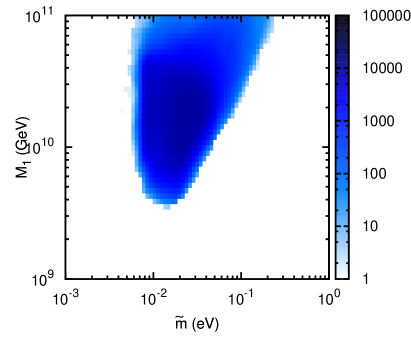
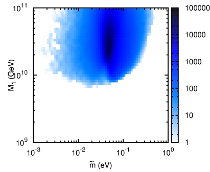
Figure I: Density of “successful” points, as a function of the lightest right-handed neutrino mass $M_{1}$ and rescaled decay rate $\tilde{m}$, assuming $\lambda_{3}\sim 1$ and $\lambda_{2}/\lambda_{1}\sim\lambda_{3}/\lambda_{2}\sim 30$, for two different simulations: NH and $\tan\beta=50$ (left), and IH and $\tan\beta=2$ (right). “Successful” points have $Y_{B}>4~{}10^{-11}$, and $BR(\mu\to e\gamma)$ and $BR(\tau\to\ell\gamma)$ an order of magnitude below the current bounds. See section 6.3.

With the parametrisation described in section 6.3, the MCMC easily finds larger values of $M_{1}$ and $\tilde{m}$, than the “tuned” points found analytically in Section 5. This preference for larger $M_{1}$ is expected, because the baryon asymmetry and right-handed neutrino masses are strongly correlated, see Fig. II and eqn (21).

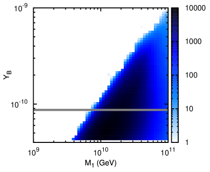
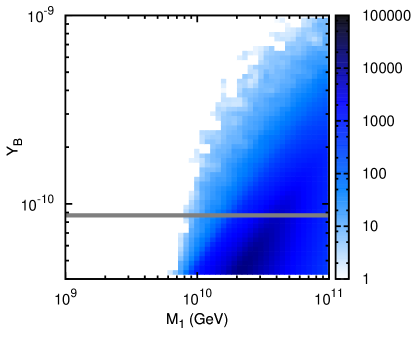
Figure II: Density of “successful” points, as a function of the baryon asymmetry and the lightest right-handed neutrino mass, assuming $\lambda_{3}\sim 1$ and $\lambda_{2}/\lambda_{1}\sim\lambda_{3}/\lambda_{2}\sim 30$, for two different simulations: NH and $\tan\beta=50$ (left), and IH and $\tan\beta=2$ (right). “Successful” points are defined as for Figure I.

Nonetheless, as illustrated in Fig.III, the MCMC succeeded in finding points at lower $M_{1}$, with a steeper hierarchy in the yukawas $\lambda_{3}\sim 1$, $\lambda_{2}/\lambda_{1}\sim 100$ and $\lambda_{3}/\lambda_{2}\sim 50$. The difficulties of finding these tuned points are discussed in section 6.4.

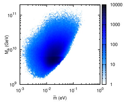
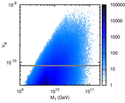
Figure III: Density of “successful” points, as a function of the lightest right-handed neutrino mass $M_{1}$ and rescaled decay rate $\tilde{m}$, on the left-side, and between the baryon asymmetry and the lightest right-handed neutrino mass, on the right-side. We assume here $\lambda_{3}\sim 1$ and $\lambda_{2}/\lambda_{1}\sim 100$ and $\lambda_{3}/\lambda_{2}\sim 50$, for a NH in the light neutrinos and $\tan\beta=2$. “Successful” points are defined as for Figure I.

The importance of the $\sim 2$ decrease in $M_{1}$ and $\tilde{m}$, at the tuned points, is unclear to us: the cosmological bound is on $T_{RH}$, rather than $M_{1}$. Since in strong washout, an equilibrium population of $N_{1}$ can be generated for $T_{RH}\mathrel{\vbox{\hbox{$>$}\nointerlineskip\hbox{$\sim$}}}M_{1}/5$, the points found by the MCMC at $M_{1}\sim 10^{10}$ GeV, could perhaps generate the BAU at the same $T_{RH}$ as the analytic points. In any case, we see in Fig.II that the fraction of points with big enough $Y_{B}$ is very sensitive to $M_{1}$, and therefore to details of the complicated reheating/preheating process.

In Fig. IV, we show density plots of the points resulting from our Markov Chains, corresponding to the the yukawa hierarchy $\lambda_{2}/\lambda_{1}\sim\lambda_{3}/\lambda_{2}\sim 30$, with $\lambda_{3}\sim 1$, for normal hierarchy (NH) of the light neutrino masses and $\tan\beta=2$, and for inverse hierarchy (IH) and $\tan\beta=50$. In Fig. VII (plot on the left) we show a density plot in the $\delta-\beta$ plane for $\tan\beta=2$, NH and the steeper hierarchy $\lambda_{2}/\lambda_{1}\sim 100$, $\lambda_{3}/\lambda_{2}\sim 50$ and $\lambda_{3}\sim 1$. From those plots we see that, for any value of the phases $\delta$, $\alpha$ and $\beta$ our conditions are satisfied. The analytic results of Section 5 agree with this. Thus, we can conclude that the baryon asymmetry of the universe is insensitive to the low energy PMNS phases, even in the “best case” where we see MSUGRA-mediated lepton flavour violating processes. For completeness we also show correlation plots between the generated BAU and the three low energy phases in Fig.V. The low energy observables do not depend on $\tan\beta$, because we assume the $(g-2)_{\mu}$ discrepancy is due to slepton loops, and we use it to normalise the LFV rates (see Eqn. 15). On the contrary, the value of $\tan\beta$ is relevant in leptogenesis because it changes the number of distinguishable flavours. However, as we can see comparing plots for small/large $\tan\beta$, the value of $\tan\beta$ does not change our conclusions.

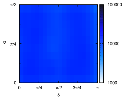
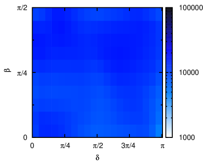
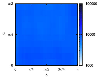
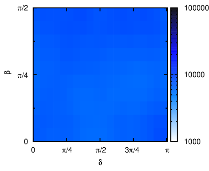
Figure IV: Density plots in the plane of the low energy phases $\delta-\alpha$ and $\delta-\beta$ in models with $\lambda_{3}\sim 1$ and $\lambda_{2}/\lambda_{1}\sim\lambda_{3}/\lambda_{2}\sim 30$. Upper plots correspond to a simulation with NH and $\tan\beta=50$, and lower plots to IH and $\tan\beta=2$. “Successful” points are defined as for Figure I.

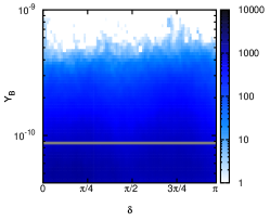
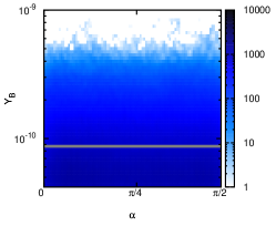
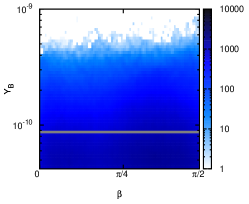
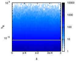
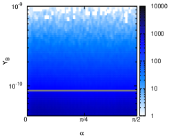
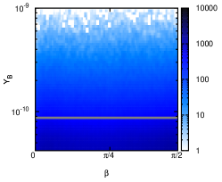
Figure V: Density of “successful” points, as a function of the BAU and the low energy phases in models with $\lambda_{3}\sim 1$ and $\lambda_{2}/\lambda_{1}\sim\lambda_{3}/\lambda_{2}\sim 30$. Upper plots correspond to a simulation with NH and $\tan\beta=50$, and the lower plots to IH and $\tan\beta=2$. “Successful” points are defined as for Figure I.

In Figs.VI and VII (plot on the right), we plot the contribution to the electric dipole moment of the electron, arising in the MSUGRA seesaw with real soft parameters at the high scale. For both low and large $\tan\beta$, points from our MCMC generate an electron EDM $\mathrel{\vbox{\hbox{$<$}\nointerlineskip\hbox{$\sim$}}}10^{-30}e$cm. This agrees with the results of [29, 35, 20].

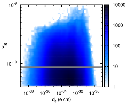
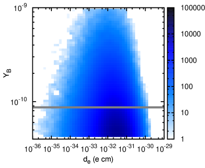
Figure VI: Density of “successful” points, as a function of the baryon asymmetry and the electron EDM generated by neutrino yukawas in models with $\lambda_{3}\sim 1$ and $\lambda_{2}/\lambda_{1}\sim\lambda_{3}/\lambda_{2}\sim 30$. The left panel corresponds to a simulation with NH and $\tan\beta=50$, and the right panel to IH and $\tan\beta=2$. “Successful” points are defined as for Figure I.

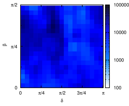
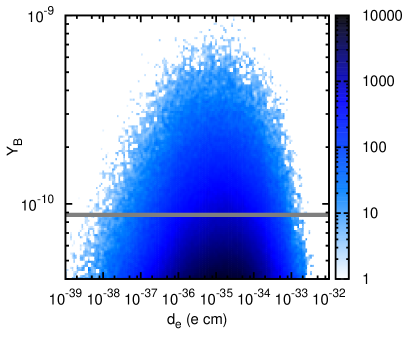
Figure VII: Density plot in $\delta-\beta$ plane and correlation between the baryon asymmetry and the electron EDM generated by neutrino yukawas. We assume here $\lambda_{3}\sim 1$, $\lambda_{2}/\lambda_{1}\sim 100$ and $\lambda_{3}/\lambda_{2}\sim 50$, for a NH in the light neutrinos and $\tan\beta=2$. “Successful” points are defined as for Figure I.

8 Summary

The aim of this work was to study whether the baryon asymmetry produced by thermal leptogenesis was sensitive to the “low energy” phases present in the leptonic mixing matrix $U_{PMNS}$. We considered the three generation type-I supersymmetric seesaw model, in the framework of MSUGRA with real soft parameters at the GUT scale, and required that it reproduces low energy neutrino oscillation data, generates a large enough baryon asymmetry of the Universe via flavoured leptogenesis and induces lepton flavour violating rates within a few orders of magnitude of current bounds. We then enquired whether a preferred range for the low energy PMNS phases $\delta$ and $\beta$ can be predicted.

We used a “left-handed” bottom-up parametrisation of the seesaw. Our parameter space scan was performed by a Monte Carlo Markov Chain (MCMC), which allows to efficiently explore high-dimensional spaces. It prefers to find the right-handed neutrino mass $M_{1}\mathrel{\vbox{\hbox{$>$}\nointerlineskip\hbox{$\sim$}}}10^{10}$ GeV, but can also find successful points with a smaller $M_{1}$ if it takes small steps in the relevant area of parameter space. In this area, we can also show analytically that the baryon asymmetry is insensitive to the PMNS phases.

We have checked that there is no correlation between successful leptogenesis and the low energy CP phases. That is: for any value of the low energy phases, the unmeasurable high energy parameters and the still unmeasured $m_{1}$ and $\theta_{13}$ can be arranged in order to have successful leptogenesis and LFV rates in the next round of experiments. The analytic estimates indicate that this result will still be true even if $m_{1}$ and $\theta_{13}$ are measured and fixed to their experimental values. Finally, we have estimated, for each point in our chains, the contribution of the complex neutrino Yukawa couplings to the electric dipole moment of the electron. As expected, we find it to be $\mathrel{\vbox{\hbox{$<$}\nointerlineskip\hbox{$\sim$}}}10^{-30}e$cm, just beyond the reach of next generation experiments.

Appendix A Fine tuning of the analytic points

In this Appendix, we estimate the fine-tuning of the points discussed in section 5, with respect to the parametrisation of section 4, which is used by the MCMC.

We do this in two steps. First, in the parametrisation of section 5, we estimate the $3\times 3$ matrix $W^{\dagger}=U^{\dagger}V_{L}^{\dagger}$ which diagonalises $m$ in the basis where $\lambda\lambda^{\dagger}$ is diagonal. Approximating this diagonal Yukawa basis to be the one where $\hat{\Lambda}\hat{\Lambda}^{\dagger}$ is diagonal, we obtain:

$$W^{\dagger}=[\delta W]^{\dagger}\left[\begin{array}[]{cc}1&~{}0~{}~{}~{}0\\ \begin{array}[]{c}0\\ 0\\ \end{array}&\hat{W}\end{array}\right]$$ (42)

where $[\delta W]^{\dagger}$ is the small rotations that rediagonalise $m=(\Delta_{ij}+\hat{D}_{\kappa})v_{u}^{2}$, and $\Delta_{ij}=\lambda_{i1}\lambda_{j1}/M_{1}$. If $W^{\dagger}$ is parametrised as in eqn (27) (but neglecting phases for simplicity), we find

$$\theta^{W}_{13} \simeq \frac{\Delta_{13}}{\kappa_{3}}\cos\hat{\theta}_{W}+\frac{\Delta_{12}}{\kappa_{2}}\sin\hat{\theta}_{W}$$ (43)

$$\theta^{W}_{12} \simeq -\frac{\Delta_{13}}{\kappa_{3}}\sin\hat{\theta}_{W}+\frac{\Delta_{12}}{\kappa_{2}}\cos\hat{\theta}_{W}$$ (44)

$$\sin\theta^{W}_{23} \simeq \sin\hat{\theta}_{W}+\frac{\Delta_{23}}{\kappa_{3}}\cos\hat{\theta}_{W}~{}~{}~{}.$$ (45)

To obtain $\lambda_{21}$ negligeable compared to $\lambda_{31}$ in eqn (33), requires no particular tuning of $\theta^{W}_{12}$ and $\theta^{W}_{13}$ with respect to $\lambda_{21}$ and$\lambda_{31}$.

The second step is to estimate the tuning required to obtain small angles $\theta^{W}_{12}$ and $\theta^{W}_{13}$ in $W^{\dagger}=U^{\dagger}V_{L}^{\dagger}$. With $V_{L}^{\dagger}$ parametrised as in eqn (27), this happens if the angles of $V_{L}$ satisfy $\theta^{L}_{ij}\simeq\theta_{ij}$ (for $i,j=12,13$). So the “tuning” required in $\theta^{L}_{12}$ and $\theta^{L}_{13}$ to obtain small $\theta^{W}_{ij}=\theta^{L}_{ij}-\theta_{ij}$ is

$$\frac{\theta^{W}_{12}}{\theta^{L}_{12}}\frac{\theta^{W}_{13}}{\theta^{L}_{13}}\simeq\frac{\tilde{m}^{2}}{m_{3}^{2}\theta_{13}}$$ (46)

This implies that $\theta_{13}^{L}$ must be tuned against $\theta_{13}$ to obtain $\theta^{W}_{13}\sim.01$. If instead $\theta_{13}\mathrel{\vbox{\hbox{$<$}\nointerlineskip\hbox{$\sim$}}}.01$, there is no particular tuning of $\theta^{W}_{13}$, and the tuning of $\theta^{W}_{12}$ with respect to $\theta^{L}_{12}$ is or order $\tilde{m}/m_{3}$.

References

- [1] P. Minkowski, Phys. Lett. B 67, 421 (1977); M. Gell-Mann, P. Ramond and R. Slansky, Proceedings of the Supergravity Stony Brook Workshop, New York, 1979, eds. P. Van Nieuwenhuizen and D. Freedman (North-Holland, Amsterdam); T. Yanagida, Proceedings of the Workshop on Unified Theories and Baryon Number in the Universe, Tsukuba, Japan 1979 (eds. A. Sawada and A. Sugamoto, KEK Report No. 79-18, Tsukuba); R. Mohapatra and G. Senjanovic, Phys. Rev. Lett. 44, 912 (1980).
- [2] M. Fukugita and T. Yanagida, Phys. Lett. B174 (1986) 45.
- [3] S. Davidson and A. Ibarra, JHEP 0109, (2001), 013. hep-ph/0104076.
- [4] G. C. Branco, T. Morozumi, B. M. Nobre and M. N. Rebelo, Nucl. Phys. B 617 (2001) 475 [arXiv:hep-ph/0107164].
- [5] S. Davidson, J. Garayoa, F. Palorini and N. Rius, arXiv:0705.1503 [hep-ph].
- [6] A. Abada, S. Davidson, F. X. Josse-Michaux, M. Losada and A. Riotto, JCAP 0604 (2006) 004 [arXiv:hep-ph/0601083]; E. Nardi, Y. Nir, E. Roulet and J. Racker, JHEP 0601, 164 (2006) [arXiv:hep-ph/0601084]; A. Abada, S. Davidson, A. Ibarra, F. X. Josse-Michaux, M. Losada and A. Riotto, arXiv:hep-ph/0605281.
- [7] M. Raidal et al., arXiv:0801.1826 [hep-ph].
- [8] S. Pascoli, S. T. Petcov and A. Riotto, Phys. Rev. D 75 (2007) 083511 [arXiv:hep-ph/0609125]. G. C. Branco, R. Gonzalez Felipe and F. R. Joaquim, Phys. Lett. B 645 (2007) 432 [arXiv:hep-ph/0609297], notice that the analysis of this paper includes only the decay of the lightest right handed neutrino, , so the excluded regions found may be allowed if the baryon asymmetry is generated by decays.
- [9] S. Pascoli, S. T. Petcov and A. Riotto, Nucl. Phys. B 774 (2007) 1 [arXiv:hep-ph/0611338].
- [10] A. Anisimov, S. Blanchet and P. Di Bari, JCAP 0804 (2008) 033 [arXiv:0707.3024 [hep-ph]].
- [11] E. Molinaro and S. T. Petcov, arXiv:0803.4120 [hep-ph].
- [12] Borzumati, Francesca and Masiero, Antonio, Phys. Rev. Lett. 57 , (1986) 961.
- [13] J. Hisano, T. Moroi, K. Tobe and M. Yamaguchi, Phys. Rev. D 53 (1996) 2442 [arXiv:hep-ph/9510309]. J. Hisano and D. Nomura, Phys. Rev. D 59 (1999) 116005 [arXiv:hep-ph/9810479].
-
[14]
S Lavignac, I Masina and C Savoy,
Phys. Lett.
B520 (2001), 269-278 . hep-ph/0106245.
Petcov, S. T. and Rodejohann, W. and Shindou, T. and Takanishi, Y.”, Nucl. Phys. B739 (2006) 208-233. hep-ph/0510404. T. Blazek and S. F. King, Nucl. Phys. B 662 (2003) 359 [arXiv:hep-ph/0211368]. - [15] S. Antusch and A. M. Teixeira, JCAP 0702 (2007) 024 [arXiv:hep-ph/0611232].
- [16] G. C. Branco, R. Gonzalez Felipe, F. R. Joaquim and M. N. Rebelo, Nucl. Phys. B 640 (2002) 202 [arXiv:hep-ph/0202030].
- [17] E. K. Akhmedov, M. Frigerio and A. Y. Smirnov, JHEP 0309 (2003) 021 [arXiv:hep-ph/0305322].
- [18] S. T. Petcov and T. Shindou, Phys. Rev. D 74 (2006) 073006 [arXiv:hep-ph/0605151].
- [19] J. R. Ellis and M. Raidal, Nucl. Phys. B 643 (2002) 229 [arXiv:hep-ph/0206174].
- [20] F. R. Joaquim, I. Masina and A. Riotto, Int. J. Mod. Phys. A 22, 6253 (2007) [arXiv:hep-ph/0701270].
- [21] D. J. C. MacKay, “Information Theory, Inference, and Learning Algorithms”, Cambridge University Press.
- [22] W. R. Gilks, S. Richardson and D. J. Spiegelhalter, “Markov Chain Monte Carlo in Practice”, Chapman and Hall.
- [23] M. Nebot, J. F. Oliver, D. Palao and A. Santamaria, Phys. Rev. D 77 (2008) 093013 [arXiv:0711.0483 [hep-ph]].
- [24] L. Calibbi, J. J. Perez and O. Vives, arXiv:0804.4620 [hep-ph].
- [25] S. Ritta and the MEG Collaboration, Nucl. Phys. Proc. Suppl. 162 (2006) 279.
- [26] A. G. Akeroyd et al. [SuperKEKB Physics Working Group], arXiv:hep-ex/0406071.
- [27] D.DeMille et al, Phys. Rev. A 61, (2000)05250; L.R. Hunter et al,Phys. Rev. A 65, (2002) 030501(R); D. Kawall, F. Bay, S. Bickman, Y. Jiang, and D. DeMille, Phys. Rev. Lett. 92 (2004) 133007.
- [28] J. P. Miller et al. [EDM Collaboration], AIP Conf. Proc. 698 (2004) 196.
- [29] Y. Farzan and M. E. Peskin, Phys. Rev. D 70, 095001 (2004) [arXiv:hep-ph/0405214].
- [30] J. Hisano and K. Tobe, Phys. Lett. B 510 (2001) 197 [arXiv:hep-ph/0102315].
- [31] K. Hagiwara, A. D. Martin, D. Nomura and T. Teubner, Phys. Lett. B 649 (2007) 173 [arXiv:hep-ph/0611102].
- [32] D. W. Hertzog, J. P. Miller, E. de Rafael, B. Lee Roberts and D. Stockinger, arXiv:0705.4617 [hep-ph].
- [33] T. Moroi, Phys. Rev. D 53 (1996) 6565 [Erratum-ibid. D 56 (1997) 4424] [arXiv:hep-ph/9512396].
- [34] M. Davier, Nucl. Phys. Proc. Suppl. 169 (2007) 288 [arXiv:hep-ph/0701163].
- [35] J. R. Ellis, J. Hisano, M. Raidal and Y. Shimizu, Phys. Lett. B 528 (2002) 86 [arXiv:hep-ph/0111324].
- [36] I. Masina, Nucl. Phys. B 671 (2003) 432 [arXiv:hep-ph/0304299].
- [37] E. Komatsu et al. [WMAP Collaboration], arXiv:0803.0547 [astro-ph].
- [38] S. Davidson, E. Nardi and Y. Nir, arXiv:0802.2962 [hep-ph].
- [39] L. Covi, E. Roulet and F. Vissani, Phys. Lett. B 384 (1996) 169 [arXiv:hep-ph/9605319].
- [40] V. A. Kuzmin, V. A. Rubakov and M. E. Shaposhnikov, Phys. Lett. B 155 (1985) 36.
-
[41]
Khlebnikov, S. Yu. and Shaposhnikov, M. E.,
Nucl. Phys.,
B308,
(1988)
885-912.
Harvey, Jeffrey A. and Turner, Michael S., Phys. Rev., D42, (1990) 3344-3349. - [42] R. Barbieri, P. Creminelli, A. Strumia and N. Tetradis, Nucl. Phys. B 575 (2000) 61 [arXiv:hep-ph/9911315].
- [43] M. Y. Khlopov and A. D. Linde, Phys. Lett. B 138 (1984) 265; J. R. Ellis, J. E. Kim and D. V. Nanopoulos, Phys. Lett. B 145 (1984) 181; J. R. Ellis, D. V. Nanopoulos and S. Sarkar, Nucl. Phys. B 259 (1985) 175; T. Moroi, H. Murayama and M. Yamaguchi, Phys. Lett. B 303 (1993) 289; M. Kawasaki, K. Kohri and T. Moroi, Phys. Lett. B 625 (2005) 7; For a recent discussion, see: K. Kohri, T. Moroi and A. Yotsuyanagi, Phys. Rev. D 73 (2006) 123511. C. Bird, K. Koopmans and M. Pospelov, arXiv:hep-ph/0703096. F. D. Steffen, arXiv:0806.3266 [hep-ph].
- [44] Buchmuller, W. and Di Bari, P. and Plumacher, M., Ann. Phys. 315 (2005) 305-351. hep-ph/0401240.
- [45] G. F. Giudice, A. Notari, M. Raidal, A. Riotto and A. Strumia, Nucl. Phys. B 685 (2004) 89 [arXiv:hep-ph/0310123].
- [46] S. Davidson and A. Ibarra, Phys. Lett. B 535 (2002) 25 [arXiv:hep-ph/0202239].
- [47] G. F. Giudice, L. Mether, A. Riotto and F. Riva, arXiv:0804.0166 [hep-ph].
- [48] M. Kawasaki, K. Kohri, T. Moroi and A. Yotsuyanagi, arXiv:0804.3745 [hep-ph].
- [49] T. Kanzaki, M. Kawasaki, K. Kohri and T. Moroi, Phys. Rev. D 75 (2007) 025011 [arXiv:hep-ph/0609246]. J. L. Diaz-Cruz, J. R. Ellis, K. A. Olive and Y. Santoso, JHEP 0705 (2007) 003 [arXiv:hep-ph/0701229].
- [50] W. Buchmuller, L. Covi, K. Hamaguchi, A. Ibarra and T. Yanagida, JHEP 0703 (2007) 037 [arXiv:hep-ph/0702184]. A. Ibarra and D. Tran, arXiv:0804.4596 [astro-ph]. K. Ishiwata, S. Matsumoto and T. Moroi, arXiv:0805.1133 [hep-ph].
- [51] S. Davidson, arXiv:hep-ph/0409339.
- [52] A. Bandyopadhyay et al. [ISS Physics Working Group], arXiv:0710.4947 [hep-ph].
- [53] M. Cirelli and A. Strumia, JCAP 0612 (2006) 013 [arXiv:astro-ph/0607086]. S. Hannestad and G. G. Raffelt, JCAP 0611 (2006) 016 [arXiv:astro-ph/0607101]. U. Seljak, A. Slosar and P. McDonald, JCAP 0610 (2006) 014.
- [54] C. Kraus et al., Eur. Phys. J. C 40 (2005) 447 [arXiv:hep-ex/0412056].
- [55] H. V. Klapdor-Kleingrothaus et al., Eur. Phys. J. A 12 (2001) 147 [arXiv:hep-ph/0103062].
- [56] J. A. Casas and A. Ibarra, Nucl. Phys. B 618 (2001) 171 [arXiv:hep-ph/0103065].
- [57] D. A. Demir and Y. Farzan, JHEP 0510 (2005) 068 [arXiv:hep-ph/0508236].
- [58] S. Davidson, JHEP 0303 (2003) 037 [arXiv:hep-ph/0302075].
- [59] O. Vives, Phys. Rev. D 73 (2006) 073006 [arXiv:hep-ph/0512160].
- [60] F. X. Josse-Michaux and A. Abada, JCAP 0710 (2007) 009 [arXiv:hep-ph/0703084].
- [61] P. H. Frampton, S. L. Glashow and T. Yanagida, Phys. Lett. B 548, 119 (2002) [arXiv:hep-ph/0208157]. W. l. Guo, Z. z. Xing and S. Zhou, Int. J. Mod. Phys. E 16, 1 (2007) [arXiv:hep-ph/0612033].
- [62] A. Ibarra and G. G. Ross, Phys. Lett. B 591 (2004) 285 [arXiv:hep-ph/0312138]. A. Ibarra, JHEP 0601 (2006) 064 [arXiv:hep-ph/0511136].
- [63] M. Maltoni, T. Schwetz, M. A. Tortola and J. W. F. Valle, New J. Phys. 6 (2004) 122 [arXiv:hep-ph/0405172], W.-M. Yao et al. (Particle Data Group), J. Phys. G 33, 1 (2006).
- [64] E. A. Baltz and P. Gondolo, JHEP 0410 (2004) 052 [arXiv:hep-ph/0407039]; M. Kunz, R. Trotta and D. Parkinson, Phys. Rev. D 74 (2006) 023503 [arXiv:astro-ph/0602378].
- [65] B. C. Allanach, C. G. Lester and A. M. Weber, JHEP 0612 (2006) 065 [arXiv:hep-ph/0609295].
- [66] L. Verde et al. [WMAP Collaboration], Astrophys. J. Suppl. 148 (2003) 195 [arXiv:astro-ph/0302218].