Biaxial nematic and smectic phases of parallel particles with different cross sections
Abstract
We have calculated the phase diagrams of one–component fluids made of five types of biaxial particles differing in their cross sections. The orientation of the principal particle axis is fixed in space, while the second axis is allowed to freely rotate. We have constructed a free-energy density functional based on fundamental–measure theory to study the relative stability of nematic and smectic phases with uniaxial, biaxial and tetratic symmetries. Minimization of the density functional allows us to study the phase behavior of the biaxial particles as a function of the cross-section geometry. For low values of the aspect ratio of the particle cross section, we obtain smectic phases with tetratic symmetry, although metastable with respect to the crystal, as our MC simulation study indicates. For large particle aspect ratios and in analogy with previous work [Phys. Chem. Chem. Phys. 5, 3700 (2003)], we have found a four–phase point where four spinodals, corresponding to phase transitions between phases with different symmetries, meet together. The location of this point is quite sensitive to particle cross section, which suggests that optimizing the particle geometry could be a useful criterion in the design of colloidal particles that can exhibit an increased stability of the biaxial nematic phase with respect to other competing phases with spatial order.
pacs:
64.70.Md,64.75.+g,61.20.GyI Introduction
The stability of thermotropic biaxial nematic phases Freiser ; Nature has been the subject of many studies in the last three decades, the driving force for this effort being their potential for use in display devices and other applications deGennes . Theoretical Freiser ; Alben ; Straley ; biblio and simulation Allen ; Romano ; Camp ; Berardi studies of a number of one– and two–component model systems have indicated that biaxiality is indeed possible in bulk nematic phases, but experimental identification is difficult and, in fact, very few positive reports have appeared in the literature Nature .
Biaxial phases are a theoretical possibility in fluids made of particles that deviate from a cylindrical shape Freiser , something that all molecules do to a larger or lesser degree. However, a biaxial particle geometry does not necessarily lead to a biaxial nematic phase: the degree of biaxiality has to be large enough, and all interactions have to be tuned optimally. Some early claims for a clear identification of a biaxial phase Malhete ; Chandrasekhar ; Praefcke were not sufficiently substantiated Luckhurst , and it has not been until recently that biaxial nematics in one–component fluids have been identified unambiguously Madsen ; Acharya (although with a very low value of the biaxial order parameter) in fluids with rigid bent–core (V–shaped) molecules. Studies on V–shaped molecules, based on simple statistical models Ferrarini ; Paulo and computer simulations Bates , have provided qualitative theoretical support for the experimental observations. However, it is difficult to isolate molecular shape as the crucial ingredient that causes biaxiality in low–mass molecular fluids, since specific interactions may play a role.
The model systems on which we focus in the present paper are hard particles, which can be thought of as idealised (and quite faithful) representations of particle interactions in colloidal (rather than molecular) fluids consisting of colloidal particles with a shape anisotropy. In fact, novel methods to synthesise colloidal metallic particles with a variety of shapes, from ellipsoids Wiley and parallelepipeds to rhombohedra and tetrapods Murphy ; Jun ; Pu , are now available, which opens up new avenues for theoretical exploration. Particularly interesting are particles with rectangular shape (parallelepipeds), since the presence of sharp edges, corners and flat sides may be the source of new types of ordering. Metallic nanorods with a rectangular cross section have been synthesised using different materials Sau ; Xiang ; Sun , and various theoretical studies using different techniques and approximations indeed point to complex phase behaviour Martinez-Raton1 ; Escobedo1 ; Escobedo2 ; Escobedo3 for particles with square cross section.
Biaxial phases in mixtures are also a possibility, as some theoretical Stroobants ; Vanakaras2 ; Varga ; Wensik and simulation Camp2 studies demonstrate; a positive identification on an experimental rod–plate system also exists Kouwer . In mixtures, difficulties are associated with competition between biaxial nematic ordering and nematic demixing transitions Vanakaras3 . The stabilisation of phases with partial (smectic phase) or complete positional order (i.e. freezing) is certainly an effect that competes strongly with the formation of a stable biaxial nematic phase in one–component fluids, so that the window of particle biaxialities where a biaxial nematic phase can exist is predicted to be very narrow Ferrarini . Hard nanorod models seem to be ideal systems to study these problems, since one can focus just on particle geometry and the effect this has on phase behaviour.
In a previous paper, Vanakaras et al. Vanakaras have presented theoretical and simulation results for a fluid of parallel hard particles with rectangular cross section of arbitrary transverse aspect ratio. The results of Vanakaras et al. indicate that indeed a biaxial nematic phase can be stabilised at the expense of the smectic phase when the rectangular cross–sectional aspect ratio is sufficiently large. Mixtures of these particles have a considerably broadened region of stability for the biaxial nematic phase with respect to the pure–fluid case, which of course implies that mixing is a general mechanism to stabilise the biaxial nematic phase in these systems.
In the present paper we revisit and extend the type of particles studied by Vanakaras et al. but consider only one–component fluids, again using the approximation that particle interactions are completely hard. Since the Onsager–type theory used by Vanakaras et al. should (by construction) only provide a gross picture of the phase equilibria, we propose a sophisticated density–functional theory that overcomes some of the defficiencies of Onsager–type theories. Although our theory can be formulated for a general mixture, we particularize here to one–component fluids of particles whose main molecular axes are assumed to point along a specified direction (nematic director) but that possess a general cross section, characterised by a second molecular axis, that can freely rotate in the plane perpendicular to the nematic director. The theory is used, subject to some simplifying assumptions, to study the stabilisation of nematic and smectic mesophases for a number of particle geometries having different cross-sectional areas, such as the rectangular and elliptical, among others. Our theoretical scheme can therefore assess the relative stability between uniaxial and biaxial nematic, and uniaxial and biaxial smectic phases.
Our proposal, based on the different phase diagrams presented, is that, by optimising the particle cross section (i.e. considering a wider range of geometries, not necessarily rectangular), one can also improve the stability range of the biaxial nematic phase in one–component fluids made of colloidal nanoparticles. A universal (i.e. independent of the type of particle) feature of the phase diagrams obtained is that the two (uniaxial and biaxial) nematic and the corresponding smectic phases (four altogether) meet at a ‘four–phase point’, also observed by Vanakaras et al. for rectangular cross sections, resulting from the convergence of the corresponding four second–order transition lines separating pairs of phases. The location of this point, which is a stability boundary for the biaxial nematic phase, depends on the particle geometry and this suggests a mechanism to enhance this stability. This result may be relevant for the design and synthesis of colloidal particles exhibiting biaxial phases. An additional prediction of our theory is that, for particles with rectangular section and low transverse aspect ratio, a further, tetratic smectic phase, possessing four-fold symmetry in the transverse plane, appears in the phase diagram, albeit in metastable form. This phase is reminiscent of the corresponding tetratic nematic phase observed in two–dimensional fluids of hard rectangles Schlacken ; Martinez-Raton0 ; Chaikin . In fact, the topology of the phase diagram in the case of rectangular areas seems to have the same limit as the corresponding hard–rectangle fluid in two dimensions at high packing fractions, a result that reflects the dimensional crossover property exhibited by the density functional.
The paper is arranged as follows. In the following section we introduce the density–functional theory, with relevant details on the numerical implementation relegated to the appendix. Sec. III contains the results for all the particle geometries considered, separating the rectangular geometry from the rest, but stressing the differences and similarities in phase behaviour. We end with some conclusions and perspectives for future work.
II Fundamental–measure functional for parallel particles
The system to be studied consists of a fluid of hard biaxial particles with characteristic lengths (parallel to the axis), and (both perpendicular to the axis). The cross-section (transverse) area of the particle does not vary along the long axis of the particle, which is taken to lie along the axis (primary nematic director); particles can otherwise freely rotate about this axis. Thus the fluid is described in terms of the density profile , with the azimuthal angle of the particle second axis with respect to a fixed direction in the transverse plane (secondary nematic director). Since the long axis is fixed, a trivial scaling along this direction follows, and the phase behaviour is not going to depend on ; however, we expect a strong dependence on the particle transverse aspect ratio ( being the larger size, along the particle second axis).
We have chosen five different transverse sections, having symmetries as shown in Fig. 1: rectangle (R), semi–discorectangle (SDR, consisting of a rectangle capped with only one semi–disc in one of their ends), discorectangle (DR, obtained from the previous one by adding another semi–disc at the other end), ellipse (E), and deltoid (D, composed of an isosceles triangle and its reflection through its common base). Note that both the latter and the rectangular geometries degenerate into a square when , while ellipses and disco–rectangles both have a disc as a limit. Finally, the minimum value of aspect ratio for SDR is , corresponding to a semi-circle (see Fig. 1).

In the following we obtain a fundamental–measure density functional for the smectic phase of a fluid composed of biaxial particles with a given cross section (in the sense explained above) in the approximation that the particle long axes are parallel. For this purpose we will adopt the projecting procedure to construct a functional for such a three–dimensional fluid starting from the corresponding two–dimensional functional for particles with the same section. Details of this formalism are given in Refs. Cuesta and Capi .
Since we consider the smectic as the less symmetric liquid-crystalline phase in the present calculations, the corresponding two-dimensional particles are not assumed to exhibit any spatial ordering in the (transverse) plane and, therefore, the excess part of the free–energy density can be constructed from scaled–particle theory (SPT) [the uniform limit of most fundamental–measure functionals] by (i) making the density profiles depend only on the –coordinate, and (ii) defining two weighted densities, namely the local packing fraction,
| (1) |
where and is the cross-section area of the particle, and the two–particle weighted density
| (2) | |||||
where and we defined , with the excluded area between two cross sections. Thus, we obtain the following expression for the generating function of the excess free–energy density Cuesta :
| (3) |
Using the projecting procedure Cuesta ; Capi , the excess part of the three–dimensional free–energy density can be obtained using the formula
| (4) |
resulting in
| (5) | |||||
where the one–body weighted density is defined as
| (6) |
while a new two–particle weighted density is obtained as
| (7) |
The excess part of the free–energy functional for the smectic phase is then obtained as
| (8) |
with given by Eqn. (5), being the smectic period. The ideal part is given by
| (9) |
with the thermal volume. This ends the description of the theoretical tools that will be used to study the phase behavior of biaxial particles with different geometries. The equilibrium state of the system follows from minimisation of the total free energy density . The minimisation will be performed numerically, using a variational procedure, and adopting two different approximations for the parameterizations of the smectic density distribution (both of which obviously contain the correct one–particle distribution of the higher–symmetry phases). These parameterizations are described in detail in Appendix A.
III Results
This section is divided into two parts. In Sec. III.1 we describe in detail the results obtained for a system of hard biaxial parallelepipeds (rectangular cross section), while in Sec. III.2 we present the phase diagrams obtained for the other cross sections, stressing the most important differences in phase behavior. The phases found in the phase diagrams and the notations used are: uniaxial nematic (N), biaxial nematic (NB), tetratic nematic (NT), uniaxial smectic (Sm), biaxial smectic (SmB), and tetratic smectic (SmT). As shown later, the main conclusion that can be drawn for this study is that the variation of the cross–sectional geometry has a dramatic impact on the relative stability of the NB phase. This in turn suggests a relatively simple criterion, useful in the design of colloidal particles, to enhance the stability of the biaxial nematic phase with respect to non–uniform phases (such as the different smectic phases considered here). The underlying mechanism is alternative to that observed by Vanakaras et al. Vanakaras , where an increase of the NB stability follows by mixing two species with different sizes.
III.1 Hard biaxial parallelepipeds
Here the cross section is a rectangle with aspect ratio . We begin with a comparison between our theoretical model and standard isobaric Monte Carlo (MC) simulations conducted on systems of biaxial parallelepipeds with their long axes parallel to the axis. These systems require long times to equilibrate, so simulations in excess of sweeps per particle are needed. The main goal here is to make the comparison at the level of the equation of state (EOS), and for this purpose we chose , i.e. a small value of the aspect ratio (since this is a harder test for the theory than a large value). Minimisation of the functional was done using the decoupling approximation (see Sec. A.1), which gives exact results for the simple Sm symmetry, with no in–plane orientational ordering, but is only approximate when in–plane order builds up. As we cover the N and Sm phases, ranging from small to high densities (but always below the Sm-SmT,B transition), we have used the Gaussian parameterization proposed in Sec. A.2.
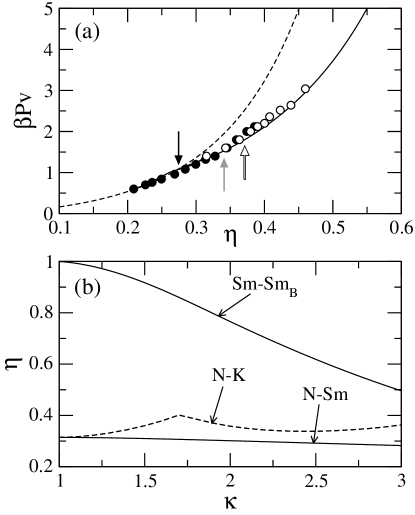
The resulting EOS, pertaining to the N and Sm branches, is shown in Fig. 2(a), along with the simulation results. First, we comment on the latter. A compression run (filled circles) was performed from the low-density nematic phase. At small–amplitude density waves began to develop, which gave rise to a fully developed smectic density distribution at (the ‘pretransitional’ modulation is probably due to the small system size along the direction). The smectic structure exhibits no in–plane order of any kind (either translational or orientational), and thus can be identified as a standard Sm phase. However, at some kind of translational order sets in, resulting in defected density distributions along , still without any orientational order in the plane. These structures may result from a tendency of the system to develop crystalline order; the fairly low value of packing fraction at which this phenomenon occurs suggests that a plastic solid phase (with particles located at the nodes of a 3D lattice, but with their second axes randomly oriented) may be involved. An expansion run (open circles in Fig. 2(a) from a perfect (biaxial) crystal at high packing fraction also produces such defected structures and does not help to clarify the situation. However, the suggestion that a plastic solid might be stabilised is indirectly supported by theoretical calculations of the spinodal to a crystal phase (K), to be presented below. The main conclusion from the present simulation study is that the window of smectic stability, , is relatively small for moderate aspect ratios. Further study is required to obtain a more quantitative picture of the phase behaviour of this system in the crystal region. In any case, one can see that the comparison between theory and simulation is fair, as far as the value of the pressure is concerned. The location of the N–Sm spinodal point as predicted by simulations is while the theory gives a value of ; this is reasonably close to the simulation result.
Our theory does not make any prediction on the transition to a crystalline phase; in fact, the extension of the present model to include columnar or crystalline ordering is not a trivial task. Even if an approximate functional could be proposed, its numerical minimisation would require huge numerical work. Therefore, in an effort to elucidate the system behaviour observed in the simulations for , we have performed a stability analysis in the framework of the restricted–orientation approximation (Zwanzig approach) to estimate the location of the N–K phase transition. The approximation involves a constraint on the orientation of the particle second axis to lie parallel to either the or axes. In this context, a fundamental–measure density functional was obtained in Ref. Cuesta , which can be applied to study phases with any spatial symmetry, in particular the crystal.
Fig. 2(b) is the phase diagram for hard parallelepipeds with small aspect ratios (between 1 and 3), as obtained from the Zwanzig approach. The continuous curves are the N-Sm and Sm-SmB spinodals, while the dashed curve is the spinodal instability in the N phase with respect to crystal fluctuations; these fluctuations are seen to correspond to a plastic solid, as suggested by the simulations. As can be seen from the figure, for the particular case , the packing–fraction interval between the N-Sm and N-K spinodals is , a result consistent with the simulations. However, this result is to be taken with care, because the Sm-K transition is expected to be of first order (since both phases have different symmetries) and, consequently, the bifurcation analysis from the N to K phase is but a gross estimate for the location of this transition. All we can say for certain is that the K phase bifurcates from the nematic at a packing fraction above (but close to) the N-Sm transition (although it is possibly metastable within some density interval after bifurcation). These results also show that, for small aspect ratios, the SmB phase is unstable with respect to the K phase.
For higher aspect ratios (for which we have not performed simulation studies), in particular for , we have found that the SmB phase is stabilized at low values of the packing fraction. To obtain the phase behavior for this particular case, we have taken advantage of the fact that the mean density is relatively small and, therefore, we have used the Fourier transform parametrization of Sec. A.3, which gives a quasi–exact representation of the true density profile (numerical convergence is guaranteed in this regime of ). The results are shown in Fig. 3 (a), where the free–energy density of the N, Sm and SmB phases is plotted as a function of the packing fraction. The system exhibits a second–order N–Sm transition, a relative small window of Sm stability, and then a continuous Sm–SmB transition, the latter being the stable phase for higher densities (up to the freezing transition). Thus, the two–dimensional orientational ordering of the particle second axis appears in a continuous fashion with increasing density. In Fig. 3 (b) the smectic period is plotted as a function of packing fraction for both types of smectic phases. It is interesting to note that the period of the SmB phase decreases very slowly with density, compared with the corresponding behaviour in the Sm phase.

With the aim to understand the non–uniform spatial and orientational correlations in the SmB phase, we have plotted in Fig. 4 the evolution of the density and the biaxial order parameter (see A.3) profiles with the mean packing fraction . While the density inhomogeneities build up with packing fraction, the order parameter profile, although globally increasing, becomes flat as a function of with increasing . Also, the profiles are out of phase, i.e. particles at smectic layers have a slightly lower orientational order than those situated at the interstitials. This is an interesting structural feature that points to a non–trivial coupling between layers via interstitial particles. However, this weak effect becomes less and less relevant as increases, as revealed by the function becoming practically constant as a function of . The latter fact justifies a posteriori the use of the decoupling approximation to study the SmB phase and, probably, also other phases, such as the SmT phase that appears at higher densities and small values of .

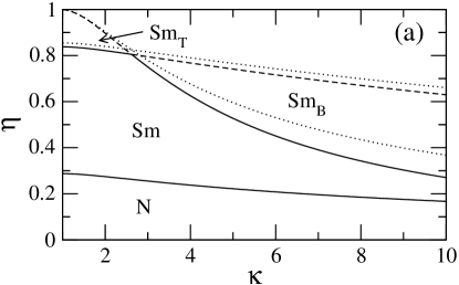
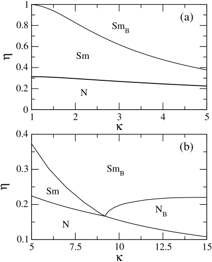
To calculate the global phase diagram we have used two approximations: the decoupling approximation with a Gaussian parameterization of for , and the Fourier–transform parametrization of the complete function for . This choice is motivated by the dependence of the numerical criterion for convergence, in the minimization routines, on the value of . The phase diagram is plotted in Figs. 5 (a) and (b). For small aspect ratios, , we find a N–Sm transition at low densities, the Sm phase being stable up to , beyond which the fluid exhibits a continuous transition to a SmT phase. This transition was calculated using Eq. (20) with . As described previously, the SmT phase consists of smectic layers in which the second particle axes (parallel to the smectic planes) point, with equal probability, along two mutually perpendicular directions (secondary nematic directors); within our approximation, the orientational distribution function fulfills the symmetry . This phase is sandwiched between the Sm and the SmB phases. Although we have not calculated numerically the location of the SmT-SmB transition, it can be approximated, as noted in a previous work Martinez-Raton0 , by the N–SmB spinodal extended to small values of [the dashed curve of Fig. 5 (a)].
The Sm-SmT phase transition can be preempted by a transition to a crystalline phase with tetratic symmetry. Nevertheless, we have shown the high density part of the phase diagram with only one-dimensional periodic phases included. As we will see later, these results are very useful for testing the performance of the present functional in the description of highly inhomogeneous fluids. Further, for aspect ratios in the range , the window of Sm stability (between the N and the SmB phases) decreases with , disappearing altogether at , the point where the N–Sm and Sm–SmB spinodals meet. This point was calculated using Eqns. (28)–(29), with the inverse of the structure factor given by Eqn. (16). For higher values of the N phase exhibits a second–order transition to the NB phase at a packing fraction calculated through Eqn. (28). On further increasing the density, there is a continuous transition between the NB and SmB phases. The NB–SmB and the N–NB spinodals meet at the point mentioned in the introduction, which will be called four–phase point Vanakaras since four different spinodals meet at the same point in the phase diagram. It is interesting to note that the transition between the NB and SmB phases is reentrant in an interval of aspect ratios just below the four–phase point. This is a genuine prediction of our theory, since Onsager theory predicts a monotonic phase boundary between these two phases Vanakaras .

It should be noted that our prediction for the location of the four–phase point at , using our density–functional approximation, is to be contrasted with the value reported in Ref. Vanakaras , where a second–virial Onsager theory was used instead. The MC simulations carried out in Ref. Vanakaras seem to confirm this latter value. However, this apparent agreement should be taken with some caution. First, Onsager theory is known to give a poor picture of the N–Sm transition due to the misrepresentation of density correlations. Also, excluded–volume effects underlying in–plane orientational ordering are probably not enough to give a quantitative description, since higher–than–two–body correlations are known to be very important in two dimensions, and the problem at hand, once smectic layers have been formed, is quasi two–dimensional in nature. On the other hand, simulations of these systems are difficult, and large system–size effects are expected. The agreement found in Ref. Vanakaras could be just fortuitous. Our approach, which includes higher–order correlations, should in principle give a more representative picture, but the situation is difficult to assess for lack of more extensive computer simulations and theoretical studies. For example, our theory gives only an approximate value for the third virial coefficient and, as shown in Ref. three-body , this coefficient is of the same order of magnitude as the second one for two-dimensional particles (the particle cross sections) in the the limit . Thus, for high aspect ratios our theory can deviate from the Onsager theory. A third–virial theory, including the exact virial coefficients up to the third order, is required to improve understanding of this issue.
III.2 Other cross sections
In this section we present the phase diagrams corresponding to the other particle cross sections described at the beginning of Sec. II. As the symmetries of the different phases and the nature of their phase transitions were discussed in the preceding section, here we will concentrate only on describing the differences between the phase diagrams of the different particle geometries.

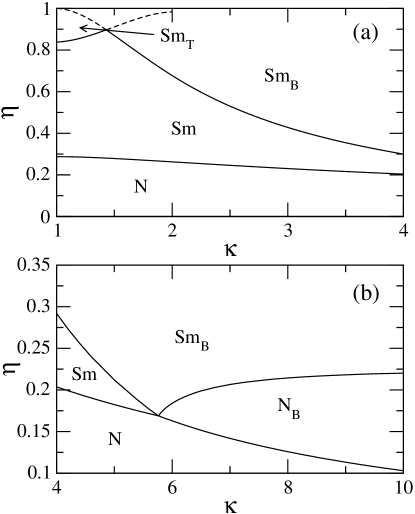
We begin by presenting the results corresponding to particles with SDR cross section (this is the only particle that does not possess head–tail symmetry). In Figs. 6 (a) and (b) we show the phase diagram. The location of the four–phase point, , is shifted to lower values of the aspect ratio, compared with the preceding case (rectangular cross section). Also, an important difference lies in the phase behaviour for small and high packing fraction. To better visualise the difference, a zoom is shown in Figs. 7 (a) and (b) in the region of SmT stability corresponding to R and SDR cross-sections, respectively.
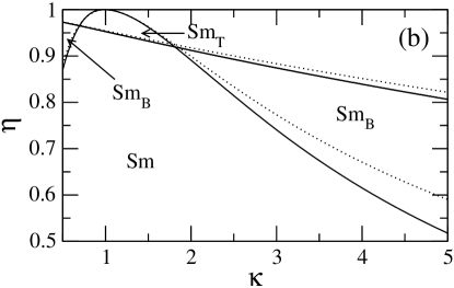
It is apparent from the figures that the stability of the SmT phase () decreases by adding a semi–disc at one end of the rectangular section. This can be explained by the increasing excluded volume involved in the T–configuration (two particles in a perpendicular configuration) when this semidisc is added. It is also interesting to note that, for , a transition between the Sm and SmB phases again occurs, due to the fact that the rectangular part is so small compared with the total area of cross section that the T–configuration is not entropically favoured. Finally, in Figs. 7 (a) and (b), the spinodals of the transitions between the isotropic phase (I) and the nematic and tetratic nematic phases of a strictly two–dimensional fluid of particles, with the same cross sections as analyzed here, are plotted. A relevant conclusion that can be drawn from the figure is the coalescence of these spinodals and those of the three–dimensional particles as packing fraction increases. This result confirms the dimensional cross–over property of the present density functional. For high the smectic phase can be considered as a collection of smectic layers where particles are perfectly located, and the effective interaction between particles located at different planes play a secondary role.
The phase diagrams for particles with cross sections corresponding to DR and E geometries are shown in Figs. 8 (a)-(b) and 9 (a)-(b), respectively. These two phase diagrams have the common feature that the SmT phase is absent. The four–phase points are now located at and , respectively. Finally, Figs. 10 (a)–(b) are the phase diagrams of particles with D section. Now at high packing fractions, and for aspect ratios in the range , the Sm phase exhibits a second–order transition to a SmT phase. However, the spinodal for this transition [] is an increasing function of , which can be explained by the change of particle geometry with . The deltoid in the limit coincides with a square; departure from this limit by increasing involves a change in the angle between the adjacent sides of the deltoid from its initial value of 90∘ and, as a consequence, the T–configuration of a pair of particles (which is characteristic of the tetratic symmetry) is less favoured.
An additional feature that depends on the particle geometry is the occurrence of reentrant behaviour in the transition between the NB and SmB phases. This behaviour is clearly associated with the rectangular nature of the particle shape, as it only appears in the phase diagrams of R and SDR particles, and much more pronounced in the former. Since both phases exhibit biaxial order, and the reentrant transition involves nematic to smectic ordering (or vice versa), the effect is the result of a nontrivial coupling between spatial ordering along the direction and angular ordering in the transverse plane.
To explain the evolution of the four–phase points with the change in particle geometry we resort to Fig. 11, where the ratio between the coefficients and is plotted for different cross sections. This ratio is a measure of the relative reduction in excluded volume, or relative gain in free volume, when the particles are orientationally ordered along the nematic director. As can be seen from the figure, this gain increases by modifying the particle sections in the sequence R, SDR, DR, E and D. This in turn explains the sequence found in the location of the four–phase point, namely the NB phase appears, for the first time, for the particle geometry that maximizes the gain in free volume associated to the orientational ordering of the second particle axis.

IV Conclusions
In the present article we have analysed the phase behaviour of models of particles that exhibit biaxial liquid–crystalline order, with an emphasis on biaxial nematic phases. The models consist of hard particles with their principal axes parallel to each other, and such that the cross section along this common axis is constant while the secondary axis associated with this cross section can otherwise rotate freely in the plane. The positive identification of a biaxial nematic phase requires that its stability be compared with that of competing phases with spatial order, such as the smectic phase. In order to incorporate these phases into the theoretical scheme, a proper treatment of correlations has to be done. Since Onsager–type theories present severe defficiencies in this respect, we have developed a density functional, based on fundamental–measure theory, which makes a more appropriate treatment of correlations at high densities. The theory has been applied to study nematic and smectic phases with different orientational symmetries, such as the biaxial and tetratic symmetries, and the global phase diagrams, for particles with five different cross sections.
As our first and most important result, we have obtained the evolution in phase behavior with particle geometry. For small aspect ratios and for R, SDR, DR and D–type sections, we have found a smectic phase with tetratic symmetry. The spinodals of the phase transitions between Sm and SmB,T phases, at high packing fractions, are similar to those corresponding to phase transitions between isotropic and uniaxial or tetratic nematic phases of a strictly 2D fluid composed of particles with the same cross section. This result confirms the dimensional cross–over property of the functional. However, the SmT phase is preempted by the crystalline phase, as the MC simulations seem to show. All the phase diagrams for large values of have a common feature, consisting in the presence of a four–phase point at which the four spinodals corresponding to the second–order N–Sm, N–NB, Sm–SmB and NB–SmB transitions meet. By studying the location of this point as a function of particle geometry, we have obtained a procedure to increase the NB–phase stability, which might be useful in the design and synthesis of colloidal particles exhibiting a transition to this phase. In particular, the deltoid seems to be the cross section that favours the NB stability most. Note that this idea is alternative to that proposed in Ref. Vanakaras , which consists in mixing two species with the same cross section but different particle lengths.
The density functional proposed in this work can be used in a variety of situations, in particular, to study interfacial problems and the effect of confinement (for example in slit geometry) on the stability of different smectic phases of a fluid composed by biaxial particles. This study we leave for future work.
Acknowledgements.
Y.M.-R. gratefully acknowledges financial support from Ministerio de Educación y Ciencia (Spain) under a Ramón y Cajal research contract and the MOSAICO grant. This work is part of the research projects Nos. FIS2005-05243-C02-01 and FIS2007-65869-C03-01, also from Ministerio de Educación y Ciencia, and grant No. S-0505/ESP-0299 from Comunidad Autónoma de Madrid (Spain). Support from the Spanish–Hungarian ‘Integrated Actions’ programme under grant Nos. HH-2006-0005 is also acknowledged.Appendix A Density profile parameterizations
In A.1 we describe the decoupling approximation and the corresponding expressions for free energy and structure factor. In A.2 a variational density profile, based on Gaussian trial functions, is proposed which, together with the decoupling approximation, allows to calculate the high density region of the phase diagrams. Finally, in A.3 a truncated Fourier expansion of the density profile is introduced; this parameterization is nearly exact for the description of smectic phases, but has the pitfall that it can only be used for low values of the mean densities due to the poor numerical convergence of the minimization procedure.
A.1 Decoupling approximation
We adopt the usual decoupling approximation for the density profile:
| (10) |
with the orientational distribution function. As its name indicates, this approach decouples spatial and angular variables, which implies –independent orientational order in the smectic phase. In turn this means that the biaxial order parameters, defined by
| (11) |
with for uniaxial and for two–dimensional tetratic symmetries, respectively, are constant within a smectic period.
Inserting (10) into (5), we obtain
| (12) | |||||
where the double angular average
has been defined. Also, the dimensionless quantity was introduced. Using the Fourier expansion of the orientational distribution function,
| (14) |
we obtain, for the double angular average,
| (15) |
with . The Fourier coefficients are given in Appendix B for all the particle sections studied (note that for all the geometries, except for SDR, the only one that breaks the head–tail symmetry; see discussion on the consequence of this in Sec. A.3).
The continuous N–Sm transition can be calculated from the divergence of the inverse structure factor , calculated from the Fourier transform of the direct correlation function ; the latter is obtained from the second functional derivative of with respect to the density profile. Within the decoupling approximation, this results in
| (16) |
with , , , and where the double angular average is to be evaluated with , which gives the coefficient . The equation , together with , must be solved for and at the absolute minimum of .
A.2 Gaussian parametrization
We adopt the following parameterized density profile:
| (17) |
i.e. a sum of normalized Gaussian peaks. This normalized form guarantees that , with the mean smectic density. Insertion of (17) into (1) and (6) gives
| (18) | |||||
| (19) | |||||
with the standard error function. For smectic symmetry, and without orientational ordering parallel to the second nematic director, the expressions for with (isotropic distribution function) are analytic functions of the particle characteristic lengths and are provided in Appendix B for all the geometries considered. We minimize the resulting free–energy density with respect to the Gaussian parameter and the smectic period for a fixed mean packing fraction . Varying and repeating the above procedure, we obtain the free–energy branch for the Sm phase. The (continuous) nematic–smectic transition is located at the mean packing fraction value for which . Alternatively, this transition can be calculated from the divergence of the inverse structure factor, defined by (16).
To calculate the second–order transitions between the Sm and the biaxial smectic (SmB) or tetratic smectic (SmT) phases, we have used a bifurcation analysis in which the orientational distribution function near the bifurcation point is approximated as ( and for the uniaxial and tetratic symmetries, respectively). After insertion of this expression into the free–energy functional obtained from the decoupling approximation (see Sec. A.1), we obtain the following expression for the free–energy difference per particle () between the SmB (or SmT) and Sm phases:
| (20) | |||||
The spinodal curves ( as a function of ) are then calculated as the solution of the equation for , where and are those values obtained from the minimization of the free–energy density of the Sm phase with respect to the Gaussian parameter and the smectic period .
A.3 Fourier parameterization and calculation of spinodals
The density profile is now parameterized by a truncated Fourier expansion:
| (21) |
where is the wave number. The latter, together with the Fourier amplitudes , span the space of minimization variables. The zeroth–component Fourier amplitude is set equal to unity, i.e. . Inserting the expression (21) into the definitions of all the one–particle weighted densities, Eqns. (1) and (6), we obtain
| (22) | |||||
| (23) |
with . Also, we obtain the following expressions for the two-particle weighted densities (2) and (7):
| (24) | |||||
| (25) | |||||
where the coefficients for the different geometries are provided in Appendix B. The free energy is then minimised with respect to the Fourier amplitudes and to the wave vector . In practice we needed about 50 Fourier components with and .
In connection with the Fourier expansion for the density (21) and the corresponding expansions for the weighted densities (24) and (25), we must note that only coefficients of the excluded area with even index, , have been taken into account. This is justified for particles with head–tail symmetry, as for these particles. However, for SDR particles, which do not exhibit this symmetry, one has . Since, for the nematic phase, or for the smectic phase in the framework of the decoupling approximation, we have , the free–energy minimization with respect to the Fourier amplitudes always gives . However, if the coupling between spatial and orientational degrees of freedom is properly taken into account, products of the form , with odd , do appear in the expansions (24)–(25) for SDR particles. These coefficients could be negative, and in principle this could result in equilibrium values , i.e. in smectic phases with in–plane polar structure in their density profiles . We expect terms of this type not to be dominant for large , and therefore we have neglected these terms in the calculations for SDR particles, in the hope that the topology of the phase diagram near the four-phase point is not greatly affected by this approximation.
A measure of the local orientational order is given by the order parameters
| (26) | |||||
with for the uniaxial order and for the tetratic order; here the relation should be used.
The second order N–NB transition can be calculated using a simple bifurcation analysis of the free–energy difference per particle between the phases, expressed as a truncated power series in the Fourier amplitudes (retaining only the first term):
| (27) |
The non-trivial solution to the equation gives
| (28) |
The intersection between the spinodal of the N–Sm transition, calculated using
| (29) |
[with the inverse structure factor given by (16)] and the spinodal of the N–NB transition [, given explicitly by Eq. (28)] can be found by substituting (28) into (16) and solving (29) for the variables and . Using the Fourier parameterization approach the Sm-SmB transition is located at the value of for which , , and finally the NB– SmB bifurcation must fulfill the condition .
Let us now prove that the four–phase point must occur. In the neighborhood of this point, the leading order terms in the order–parameter expansion of the free-energy difference between the SmB and N phases from the Fourier parameterization approach [Eq. (21)] is
| (30) |
where the coefficient is proportional to the inverse of the structure factor , given by Eq. (16), with , while is the coefficient of the quadratic term in the expansion of the free–energy difference between the NB and N phases with respect to the Fourier amplitudes , given by Eq. (27). Other terms in the expansion, depending on powers of and beyond, are of higher order in magnitude. Thus, at this order of approximation, the smectic and orientational order parameters are decoupled. Minimization of (30) with respect to and gives the set of coupled equations
| (31) |
with the value at the absolute minimum of with respect to . These equations should be solved together for and to find the (unique) point in the – plane where the N phase becomes unstable with respect to SmB fluctuations. But note that Eqn. (31), as pointed out before, are also the equations, Eqns. (28)-(29) [obtained from the decoupling approximation], whose simultaneous solution corresponds to the point where the N-Sm and N-NB spinodal curves meet. This proves that this point is indeed a four-phase point.
Appendix B Expressions for the coefficients
In this section we provide the analytic expressions for the coefficients corresponding to all the particle transverse sections studied.
| (32) | |||||
| (33) | |||||
| (34) | |||||
with . Finally, the expression for the E geometry can be calculated only numerically from
| (36) |
with the complete elliptic integral of the second kind and where there were defined
| (37) |
For we have .
References
- (1) M. J. Freiser, Phys. Rev. Lett. 24, 1041 (1970).
- (2) G. R. Luckhurst, Nature 430, 413 (2004).
- (3) See e.g. P. G. de Gennes and J. Prost, The Physics of Liquid Crystals (Clarendon, Oxford, 1993).
- (4) R. Alben, J. Chem. Phys. 59, 4299 (1973).
- (5) J. P. Straley, Phys. Rev. A 10, 1881 (1974).
- (6) P. I. C. Teixeira, M. A. Osipov, and G. R. Luckhurst, Phys. Rev. E 73, 061708 (2006).
- (7) M. P. Allen, Liq. Cryst. 8, 499 (1990).
- (8) P. J. Camp and M. P. Allen, J. Chem. Phys. 106, 6681 (1997).
- (9) R. Berardi and C. Zannoni, J. Chem. Phys. 113, 5971 (2000).
- (10) G. R. Luckhurst and S. Romano, Mol. Phys. 40, 129 (1980).
- (11) J. Malthête, H. T. Nguyen, and A. M. Levelut, J. Chem. Soc. Chem. Commun. 1548 (1986); Corrigendum 40 (1987).
- (12) S. Chandrasekhar, B. R. Ratna, B. K. Sadashiva, and N. V. Raja, Mol. Crys. Liq. Cryst. 165, 123 (1988).
- (13) K. Praefcke, B. Kohne, D. Singer, D. Demus, G. Pelzl, and S. Diele, Liq. Crys. 7, 589 (1990).
- (14) G. R. Luckhurst, Thin Solid Films 393, 40 (2001).
- (15) L. A. Madsen, T. J. Dingemans, M. Nakata, and E. T. Samulski, Phys. Rev. Lett. 92, 145506 (2004)
- (16) B. R. Acharya, A. Primak, and S. Kumar, Phys. Rev. Lett. 92, 145506 (2004)
- (17) A. Ferrarini, P. L. Nordio, E. Spolaore, and G. R. Luckhurst, J. Chem. Soc., Faraday Trans. 91, 3177 (1995).
- (18) P. I. C. Teixeira, A. J. Masters, and B. Mulder, Mol. Crys. Liq. Cryst. Sci. Technol., Sect. A 323, 167 (1998).
- (19) M. A. Bates and G. R. Luckhurst, Phys. Rev. E 72, 051702 (2005).
- (20) B. J. Wiley, Y. Chen, J. M. McLellan, Y. Xiong, Z. Li, D. Ginger, and Y. Xia, Nano Lett. 7, 1032 (2007).
- (21) C. J. Murphy, T. K. Sau, A. M. Gole, C. J. Orendorff, J. Gao, L. Gou, S. Hunyadi, and T. Li, J. Phys. Chem. B 109, 13857 (2005).
- (22) Y. Jun, J. Seo, S. J. Oh, and J. Cheon, Coord. Chem. Rev. 249, 1766 (2005).
- (23) Z. Pu, M. Cao, J. Yang, K. Huang, and C. Hu, Nanotechnology 17, 799 (2006).
- (24) T. K. Sau and C. J. Murphy, Langmuir 21, 2923 (2005).
- (25) Y. Xiang, X. Wu, D. Liu, X. Jiang, W. Chu, Z. Li, Y. Ma, W. Zhou, and S. Xie, Nano Lett. 6, 2290 (2006).
- (26) Y. Sun, L. Zhang, H. Zhou, Y. Zhu, E. Sutter, Y. Ji, M. H. Rafailovich, and J. C. Sokolov, Chem. Mater. 19 2065 (2007).
- (27) Y. Martínez-Ratón, Phys. Rev. E 69, 061712 (2004).
- (28) B. S. John, A. Stroock, and F. A. Escobedo, J. Chem. Phys. 120, 9383 (2004).
- (29) B. S. John and F. A. Escobedo, J. Phys. Chem. B 109, 23008 (2005).
- (30) B. S. John, C. Juhlin, and F. A. Escobedo, J. Chem. Phys. 128, 044909 (2008).
- (31) A. Stroobants and H. N. W. Lekkerkerker, J. Phys. Chem. 88, 3669 (1984).
- (32) A. G. Vanakaras and D. J. Photinos, Mol. Cryst. Liq. Cryst. 299, 65 (1997).
- (33) S. Varga, A. Galindo, and G. Jackson, Phys. Rev. E 66, 011707 (2002).
- (34) H. H. Wensik, G. J. Vroege, and H. N. W. Lekkerkerker, Phys. Rev. E 66, 041704 (2002).
- (35) P. J. Camp, M. P. Allen, P. G. Bolhuis, and D. Frenkel, J. Chem. Phys. 106, 9270 (1997).
- (36) P. H. J. Kouwer and G. H. Mehl, J. Am. Chem. Soc. 125, 11172 (2003).
- (37) A. G. Vanakaras, A. F. Terzis, and D. J. Photinos, Mol. Cryst. Liq. Cryst. 362, 67 (2001).
- (38) A. G. Vanakaras, M. A. Bates and D. J. Photinos, Phys. Chem. Chem. Phys. 5, 3700 (2003).
- (39) H. Schlacken, H.-J. Mogel, and P. Schiller, Mol. Phys. 93, 777 (1998).
- (40) Y. Martínez-Ratón, E. Velasco and L. Mederos, J. Chem. Phys. 122, 064903 (2005).
- (41) K. Zhao, C. Harrison, D. Huse, W. B. Russel, and P. M. Chaikin, Phys. Rev. E 76, 040401(R) (2007).
- (42) J. A. Cuesta and Y. Martínez-Ratón, Phys. Rev. Lett. 78, 3681 (1997); J. Chem. Phys. 107, 6379 (1997).
- (43) Y. Martínez-Ratón, J. A. Capitán and and J. A. Cuesta, Phys. Rev. E 77, 051205 (2008).
- (44) Y. Martínez-Ratón, E. Velasco and L. Mederos, J. Chem. Phys. 125, 014501 (2006).