L2 Orthogonal Space Time Code for Continuous Phase Modulation

Abstract

To combine the high power efficiency of Continuous Phase Modulation (CPM) with either high spectral efficiency or enhanced performance in low Signal to Noise conditions, some authors have proposed to introduce CPM in a MIMO frame, by using Space Time Codes (STC). In this paper, we address the code design problem of Space Time Block Codes combined with CPM and introduce a new design criterion based on $L^{2}$ orthogonality. This $L^{2}$ orthogonality condition, with the help of simplifying assumption, leads, in the 2x2 case, to a new family of codes. These codes generalize the Wang and Xia code, which was based on pointwise orthogonality. Simulations indicate that the new codes achieve full diversity and a slightly better coding gain. Moreover, one of the codes can be interpreted as two antennas fed by two conventional CPMs using the same data but with different alphabet sets. Inspection of these alphabet sets lead also to a simple explanation of the (small) spectrum broadening of Space Time Coded CPM.

I Introduction

Since the pioneer work of Alamouti [1] and Tarokh [2], Space Time Coding has been a fast growing field of research where numerous coding schemes have been introduced. Several years later Zhang and Fitz [3, 4] were the first to apply the idea of STC to continuous phase modulation (CPM) by constructing trellis codes. In [5] Zajić and Stüber derived conditions for partial response STC-CPM to get full diversity and optimal coding gain. A STC for noncoherent detection based on diagonal blocks was introduced by Silvester et al. [6].

The first orthogonal STC for CPM for full and partial response was developed by Wang and Xia [7, 8]. The scope of this paper is also the design of an orthogonal STC for CPM. But unlike Wang-Xia aprroach [8] which starts from a QAM orthogonal Space-Time Code (e.g. Alamouti’s scheme [1]) and modify it to achieve continuous phases for the transmitted signals, we show here that a more general $L^{2}$ condition is sufficient to ensure fast maximum likelihood decoding with full diversity.

In the considered system model (Fig.1), the data sequence $d_{j}$ is defined over the signal constellation set

$$\Omega_{d}=\{-M+1,-M+3,\ldots,M-3,M-1\}$$ (1)

for an alphabet with $\log_{2}M$ bits. To obtain the structure for a Space Time Block Code (STBC) this sequence is mapped to data matrices $\mathbf{D}^{(i)}$ with elements $d_{mr}^{(i)}$, where $m$ denotes the transmitting antenna, $r$ the time slot into a block and $(i)$ a parameter for partial response CPM. The data matrices are then used to modulate the sending matrix

$${\bf S}(t)=\begin{bmatrix}s_{11}(t)&s_{12}(t)\\ s_{21}(t)&s_{22}(t)\end{bmatrix}\text{.}$$ (2)

Each element is defined for $(2l+r-1)T\leq t\leq(2l+r)T$ as

$$s_{mr}(t)=\sqrt{\frac{E_{s}}{T}}\operatorname{e}^{j2\pi\phi_{mr}(t)}$$ (3)

where $E_{s}$ is the symbol energy and $T$ the symbol time. The phase $\phi_{mr}(t)$ is defined in the conventional CPM manner [9] with an additional correction factor $c_{mr}(t)$ and is therewith given by

$$\phi_{mr}(t)=\theta_{m}(2l+r)+h\!\!\!\!\!\!\!\!\!\sum\limits_{i=2l+1+r-\gamma}^{2l+r}\!\!\!\!\!\!\!\!\!d_{mr}^{(i)}q(t-(i-1)T)+c_{mr}(t)$$ (4)

where $h=2m_{0}/p$ with $m_{0}$ and $p$ relative primes is called the modulation index. The phase smoothing function $q(t)$ has to be a continuous function with $q(t)=0$ for $t\leq 0$ and $q(t)=1/2$ for $t\geq\gamma T$.

Figure 1: Structure of a MIMO Tx/Rx system

The memory length $\gamma$ determines the length of $q(t)$ and affects the spectral compactness. For large $\gamma$ we obtain a compact spectrum but also a higher number of possible phase states which increases the decoding effort. For full response CPM, we have $\gamma=1$ and for partial response systems $\gamma>1$.

The choice of the correction factor $c_{mr}(t)$ in Eq. (4) is along with the mapping of $d_{j}$ to $\mathbf{D}^{(i)}$, the key element in the design of our coding scheme. It will be detailed in Section II. We then define $\theta_{m}(2l+r)$ in a most general way

$$\theta_{m}(2l+3) =\theta_{m}(2l+2)+\xi(2l+2)$$

$$=\theta_{m}(2l+1)+\xi(2l+1)+\xi(2l+2).$$ (5)

The function $\xi(2l+r)$ will be fully defined from the contribution $c_{mr}(t)$ to the phase memory $\theta_{m}(2l+r)$. For conventional CPM system, $c_{mr}(t)=0$ and we have $\xi(2l+1)=\frac{h}{2}d_{2l+1-\gamma}$.

The channel coefficients $\alpha_{mn}$ are assumed to be Rayleigh distributed and independent. Each coefficient $\alpha_{mn}$ characterizes the fading between the $\mathrm{m^{th}}$ transmit (Tx) antenna and the $\mathrm{n^{th}}$ receive (Rx) antenna where $n=1,2,\ldots,L_{r}$. Furthermore, the received signals

$$y_{n}(t)=\alpha_{mn}s_{mr}(t)+n(t)$$ (6)

are corrupted by a complex additive white Gaussian noise $n(t)$ with variance $1/2$ per dimension.

At the receiver, the detection is done on each of the $L_{r}$ received signals separately. Therefore, in general, each code block $\mathbf{S}(t)$ has to be detected by block. E.g. for a 2x2 block, estimating the symbols $\hat{d}_{j}$ implies computational complexity proportional to $M^{2}$. Now, this complexity can be reduced to $2M$ by introducing an orthogonality property as well as simplifying assumptions on the code.

Criteria for such STBC are given in Section II. In Section III, the criteria are used to construct OSTBC for CPM. In Section IV we test the designed code and compare it with the STC from Wang and Xia [8]. Finally, some conclusions are drawn in Section V.

II Design Criteria

The purpose of the design is to achieve full diversity and a fast maximum likelihood decoding while maintaining the continuity of the signal phases. This section shows how the need to perform fast ML decoding leads to the $L^{2}$ orthogonality condition as well as to simplifying assumptions, which can be combined with the continuity conditions. For convenience we only consider one Rx antenna and drop the index $n$ in $\alpha_{mn}$.

II-A Fast Maximum Likelihood Decoding

Commonly, due to the trellis structure of CPM, the Viterbi algorithm is used to perform the ML demodulation . On block $l$ each state in the trellis has $M^{2}$ incoming branches and $M^{2}$ outgoing branches with a distance

$$D_{l} =\int\limits_{2lT}^{(2l+1)T}\Big{|}y(t)-\sum\limits_{m=1}^{2}\alpha_{m}s_{m1}(t)\Big{|}^{2}\operatorname{d\!}t+\int\limits_{(2l+1)T}^{(2l+2)T}\Big{|}y(t)-\sum\limits_{m=1}^{2}\alpha_{m}s_{m2}(t)\Big{|}^{2}\operatorname{d\!}t.$$ (7)

The number of branches results from the blockwise decoding and the correlation between the sent symbols $s_{1r}(t)$ and $s_{2r}(t)$. A way to reduce the number of branches is to structurally decorrelate the signals sent by the two transmitting antennas, i.e. to put to zero the inter-antenna correlation

$$\alpha_{2}\alpha_{1}^{*}\!\!\!\!\!\!\int\limits_{2lT}^{(2l+1)T}\!\!\!\!\!\!s_{21}(t)s_{11}^{*}(t)\operatorname{d\!}t+\alpha_{1}\alpha_{2}^{*}\!\!\!\!\!\!\!\!\int\limits_{2lT}^{(2l+1)T}\!\!\!\!\!\!\!\!s_{11}(t)s_{21}^{*}(t)\operatorname{d\!}t+\alpha_{2}\alpha_{1}^{*}\!\!\!\!\!\!\!\int\limits_{(2l+1)T}^{(2l+2)T}\!\!\!\!\!\!\!s_{22}(t)s_{12}^{*}(t)\operatorname{d\!}t+\alpha_{1}\alpha_{2}^{*}\!\!\!\!\!\!\!\int\limits_{(2l+1)T}^{(2l+2)T}\!\!\!\!\!\!\!s_{12}(t)s_{22}^{*}(t)\operatorname{d\!}t=0.$$ (8)

Pointwise orthogonality as defined in [8] is therefore a sufficient condition but not necessary. A less restrictive $L^{2}$ orthogonality is also sufficient. From Eq. (8), the distance given in Eq. (7) can then be simplified to

$$D_{l} =\int\limits_{2lT}^{(2l+1)T}\!\!\!\!\!\!\!f_{11}(t)+f_{21}(t)-|y(t)|^{2}\operatorname{d\!}t+\int\limits_{(2l+1)T}^{(2l+2)T}\!\!\!\!\!\!\!f_{12}(t)+f_{22}(t)-|y(t)|^{2}\operatorname{d\!}t$$ (9)

with $f_{mr}(t)=|y(t)-\alpha_{m}s_{mr}(t)|^{2}$. When each $s_{mr}(t)$ depends only on $d_{2l+1}$ or $d_{2l+2}$ the branches can be split and calculated separately for $d_{2l+1}$ and $d_{2l+2}$. The complexity of the ML decision is reduced to $2M$. The complexity for detecting two symbols is thus reduced from $pM^{\gamma+1}$ to $pM^{\gamma}$. The STC introduced by Wang and Xia [8] didn’t take full advantage of the orthogonal design since $s_{mr}(t)$ was depending on both $d_{2l+1}$ and $d_{2l+2}$. The gain they obtained in [8] was then relying on other properties of CPM, e.g. some restrictions put on $q(t)$ and $p$. These restrictions may also be applied to our design code, which would lead to additional complexity reduction. However, this is not in the scope of this paper and is be the subject of another upcoming paper.

II-B Orthogonality Condition

In this section we show how $L^{2}$ orthogonality for CPM, i.e. $\|\mathbf{S}(t)\|^{2}_{L_{2}}=\int_{2lT}^{(2l+2)T}\mathbf{S}(t)\mathbf{S}^{H}(t)\operatorname{d\!}t=2\mathbf{I}$, can be obtained. As such, the correlation between the two transmitting antennas per coding block is cancelled if

$$\int\limits_{2lT}^{(2l+2)T}s_{1r}(t)s_{2r}^{*}(t)\operatorname{d\!}t =\int\limits_{2lT}^{(2l+1)T}s_{11}(t)s_{21}^{*}(t)\operatorname{d\!}t+\int\limits_{(2l+1)T}^{(2l+2)T}s_{12}(t)s_{22}^{*}(t)\operatorname{d\!}t=0\text{.}$$ (10)

Replacing $s_{mr}(t)$ by the corresponding CPM symbols from Eq. (4), we get

$$\!\int\limits_{2lT}^{(2l+1)T}\!\!\!\!\!\!\!\exp\!\Big{\{}j2\pi\big{[}\theta_{1}(2l+1)+h\!\!\!\!\!\!\!\sum\limits_{i=2l+2-\gamma}^{2l+1}\!\!\!\!\!\!\!d_{1,1}^{(i)}q(t-(i-1)T)+c_{1,1}(t)-\theta_{2}(2l+1)-h\!\!\!\!\!\!\sum\limits_{i=2l+3-\gamma}^{2l+2}\!\!\!\!\!\!d_{2,1}^{(i)}q(t-(i-1)T)-c_{2,1}(t)\big{]}\Big{\}}\operatorname{d\!}t+$$

$$\!\int\limits_{(2l+1)T}^{(2l+2)T}\!\!\!\!\!\!\!\exp\!\Big{\{}j2\pi\big{[}\theta_{1}(2l+2)+h\!\!\!\!\!\!\!\sum\limits_{i=2l+3-\gamma}^{2l+2}\!\!\!\!\!\!\!d_{1,2}^{(i)}q(t-(i-1)T)\!+\!c_{1,2}(t)-\theta_{2}(2l+2)-h\!\!\!\!\!\!\sum\limits_{i=2l+2-\gamma}^{2l+1}\!\!\!\!\!\!d_{2,2}^{(i+1)}q(t-iT)-c_{2,2}(t)\big{]}\operatorname{d\!}t\Big{\}}=0.$$ (11)

The phase memory $\theta_{m}(2l+r)$ is independent of time and has not to be considered for integration. Using Eq. (5) to replace phase memory $\theta_{m}(2l+2)$ of the second time slot, we obtain

$$\int\limits_{2lT}^{(2l+1)T}\!\!\!\!\!\!\exp\Big{\{}j2\pi\big{[}h\!\!\!\!\!\!\sum\limits_{i=2l+2-\gamma}^{2l+1}\!\!\!\!\!\!d_{1,1}^{(i)}q(t-(i-1)T)+c_{1,1}(t)-h\!\!\!\!\!\!\sum\limits_{i=2l+2-\gamma}^{2l+1}\!\!\!\!\!\!d_{2,1}^{(i)}q(t-(i-1)T)-c_{2,1}(t)\big{]}\Big{\}}\operatorname{d\!}t+$$

$$\exp\Big{\{}j2\pi\big{[}\xi_{1}(2l+1)-\xi_{2}(2l+1)\big{]}\Big{\}}\cdot\int\limits_{2lT}^{(2l+1)T}\!\!\!\!\!\!\!\exp\Big{\{}j2\pi\big{[}h\!\!\!\!\!\!\sum\limits_{i=2l+2-\gamma}^{2l+1}\!\!\!\!\!\!d_{1,2}^{(i+1)}q(t-(i-1)T)+c_{1,2}(t+T)-$$

$$h\!\!\!\!\!\!\sum\limits_{i=2l+2-\gamma}^{2l+1}\!\!\!\!\!\!d_{2,2}^{(i+1)}q(t-(i-1)T)-c_{2,2}(t+T)\big{]}\Big{\}}\operatorname{d\!}t =0.$$ (12)

II-C Simplifying assumptions

To simplify this expression, we factor Eq. (12) into a time independent and a time dependent part. For merging the two integrals to one time dependent part, we have to map $d_{m2}^{(i)}$ to $d_{m1}^{(i)}$ and $c_{mr}(t)$ to a different $c_{m^{\prime}r^{\prime}}(t)$. Consequently, for the data symbols $d_{mr}^{(i)}$ there exist three possible ways of mapping:

• crosswise mapping with $d_{1,1}^{(i)}=d_{2,2}^{(i)}$ and $d_{1,2}^{(i)}=d_{2,1}^{(i)}$;

• repetitive mapping with $d_{1,1}^{(i)}=d_{1,2}^{(i)}$ and $d_{2,1}^{(i)}=d_{2,2}^{(i)}$;

• parallel mapping with $d_{1,1}^{(i)}=d_{2,1}^{(i)}$ and $d_{1,2}^{(i)}=d_{2,2}^{(i)}$ .

The same approach can be applied to $c_{mr}(t)$:

• crosswise mapping with $c_{11}(t)=-c_{22}(t-T)$ and $c_{12}(t)=-c_{21}(t-T)$;

• repetitive mapping with $c_{11}(t)=c_{12}(t-T)$ and $c_{21}(t)=c_{22}(t-T)$;

• parallel mapping with $c_{11}(t)=c_{21}(t)$ and $c_{12}(t)=c_{22}(t)$.

For each combination of mappings, Eq. (12) is now the product of two factors, one containing the integral and the other a time independent part. To fulfill Eq. (12) it is sufficient if one factor is zero, namely $1+\operatorname{e}^{j2\pi\left[\xi_{1}(2l+1)-\xi_{2}(2l+1)\right]}=0$, i.e. if

$$k+\frac{1}{2}=\xi_{1}(2l+1)-\xi_{2}(2l+1)$$ (13)

with $k\in\mathbb{N}$. We thus get a very simple condition which only depends on $\xi_{m}(2l+1)$.

II-D Continuity of Phase

In this section we determine the functions $\xi_{m}(2l+1)$ to ensure the phase continuity.

Precisely, the phase of the CPM symbols has to be equal at all intersections of symbols. For an arbitrary block $l$, it means that $\phi_{m1}((2l+1)T)=\phi_{m2}((2l+1)T)$. Using Eq. (4), it results in

$$\xi_{m}(2l+1) =h\!\!\!\!\!\!\!\!\!\sum\limits_{i=2l+2-\gamma}^{2l+1}\!\!\!\!\!\!\!\!d_{m,1}^{(i)}q((2l+2-i)T)+c_{m,1}((2l+1)T)-h\!\!\!\!\!\!\!\sum\limits_{i=2l+3-\gamma}^{2l+2}\!\!\!\!\!\!\!d_{m2}^{(i)}q((2l+2-i)T)-c_{m2}((2l+1)T)\text{.}$$ (14)

For the second intersection at $(2l+2)T$, since $\phi_{m2}((2l+2)T)=\phi_{m1}((2l+2)T)$, we get

$$\xi_{m}(2l+2) =h\!\!\!\!\!\!\sum\limits_{i=2l+3-\gamma}^{2l+2}\!\!\!\!\!\!\!d_{m2}^{(i)}q((2l+3-i)T)+c_{m2}((2l+2)T)-h\!\!\!\!\!\!\!\!\!\!\sum\limits_{i=2(l+1)+2-\gamma}^{2(l+1)+1}\!\!\!\!\!\!\!\!\!\!\!d_{m,1}^{(i)}q((2l+3-i)T)-c_{m,1}((2l+2)T)]\text{.}$$ (15)

Now, by choosing one of the mappings detailed in Section III, these equations can be greatly simplified. Hence, we have all the tools to construct our code.

III Orthogonal Space Time Codes

In this section we will have a closer look at two codes constructed under the afore-mentioned conditions.

III-A Existing Code

As a first example, we will give an alternative construction of the code given by Wang and Xia in [8]. Indeed, the pointwise orthogonality condition used by Wang and Xia is a special case of the $L^{2}$ orthogonality condition, hence, their ST-code can be obtained within our framework.

For the first antenna Wang and Xia use a conventional CPM with $d_{1r}^{(i)}=d_{i}$ for $i=2l+r+1-\gamma,2l+r+2-\gamma,\ldots,2l+r$ and $c_{1r}(t)=0$. The symbols of the second antenna are mapped crosswise to the first $d_{21}^{(i)}=-d_{i+1}$ for $i=2l+2-\gamma,2l+3-\gamma,\ldots,2l+1$ and $d_{22}^{(i-1)}=-d_{i-1}$ for $i=2l+3-\gamma,2l+4-\gamma,\ldots,2l+2$. Using this cross mapping makes it difficult to compute $\xi_{m}(2l+1)$ since the CPM typical order of the data symbols is mixed. Wang and Xia circumvent this by introducing another correction factor for the second antenna

$$c_{2r}(t)\!=\!\!\sum\limits_{i=0}^{\gamma-1}(h({d_{2l+1-i}+d_{2l+2-i}})+1)q_{0}(t-(2l+r-1-i)T)$$ (16)

By first computing $\xi_{m}(2l+1)$ with Eq. (17) and then Eq. (13), we get the $L^{2}$ orthogonality of the Wang-Xia-STC.

III-B Parallel Code

To get a simpler correction factor as in [8], we designed a new code based on the parallel structure which permits to maintain the conventional CPM mapping for both antennas. Hence we choose the following mapping: $d_{m1}^{(i)}=d_{m2}^{(i-1)}=d_{i}$ for $i=2l+r+1-\gamma,2l+r+2-\gamma,\ldots,2l+r$. Then, Eq. (14) and (15) can be simplified into

$$\xi_{m}(2l+1) =\frac{h}{2}d_{2l+2-\gamma}+c_{m1}((2l+1)T)-c_{m2}((2l+1)T)$$ (17)

$$\xi_{m}(2l+2) =\frac{h}{2}d_{2l+3-\gamma}+c_{m2}((2l+2)T)-c_{m1}((2l+2)T)\text{.}$$ (18)

With this simplified functions, the orthogonality condition only depends on the start and end values of $c_{mr}(t)$, i.e.

$$k+\frac{1}{2} =c_{11}((2l+1)T)-c_{12}((2l+1)T)-c_{21}((2l+1)T)+c_{22}((2l+1)T).$$ (19)

To merge the two integrals in Eq. (12) not only the mapping of $d_{mr}^{(i)}$ is necessary but also an equality between different $c_{mr}(t)$. From the three possible mappings, we choose the repeat mapping because of the possibility to set $c_{mr}(t)$ to zero for one antenna. Hence we are able to send a conventional CPM signal on one antenna and a modified one on the second. Using Eq. (19) and the equalities for the mapping, we can formulate the following condition

$$k+\frac{1}{2}=c_{12}(2lT)-c_{12}((2l+1)T)-c_{22}(2lT)+c_{22}((2l+1)T).$$ (20)

With $c_{11}(t)=c_{12}(t)=0$, we can take for $c_{21}(t)=c_{22}(t)$ any continuous function which is zero at $t=0$ and $1/2$ at $t=T$. Another possibility is to choose the correction factor of the second antenna with a structure similar to CPM modulation, i.e.

$$c_{2r}(t)=\sum\limits_{i=2l+1-\gamma}^{2l+1}q(t-(i-1)T)$$ (21)

for ${(2l+r-1)T\leq t\leq(2l+r)T}$. With this approach, the correction factors can be included in a classical CPM modulation with constant offset of $1/h$. This offset may also be expressed as a modified alphabet for the second antenna

$$\Omega_{d_{2}}=\{-M+1+\frac{1}{h},-M+3+\frac{1}{h},\ldots,M-3+\frac{1}{h},M-1+\frac{1}{h}\}$$ (22)

Consequently, this $L^{2}$-orthogonal design may be seen as two conventional CPM designs with different alphabet sets $\Omega_{d}$ and $\Omega_{d2}$ for each antenna. However, in this method, the constant offset to the phase may cause a shift in frequency. But as shown by our simulations in the next section, this shift is quite moderate.

IV Simulations

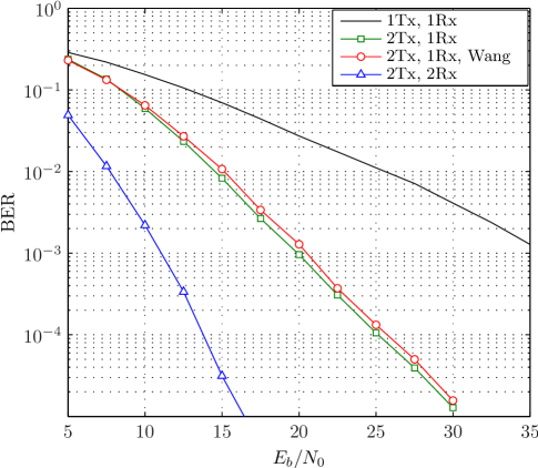
Figure 2: Simulated BER for different numbers of Tx and Rx antennas of the proposed STC and of the Wang-Xia-STC

In this section we verify the proposed algorithm by simulations. Therefore a STC-2REC-CPM-sender with two transmitting antennas has been implemented in MATLAB. For the signal of the first antenna we use conventional Gray-coded CPM with a modulation index $h=1/2$, the length of the phase response function $\gamma=2$ and an alphabet size of $M=8$. The signal of the second antenna is modulated by a CPM with the same parameters but a different alphabet $\Omega_{d_{2}}$, corresponding to Eq. (22).

The channel used is a frequency flat Rayleigh fading model with additive white Gaussian noise. The fading coefficients $\alpha_{mn}$ are constant for the duration of a code block (block fading) and known at receiver (coherent detection). The received signal $y_{n}(t)$ is demodulated by two filterbanks with $pM^{2}$ filters, which are used to calculate the correlation between the received and candidate signals. Due to the orthogonality of the antennas each filterbank is independently applied to the corresponding time slot $k$ of the block code. The correlation is used as metric for the Viterbi algorithm (VA) which has $pM$ states and $M$ paths leaving each state. In our simulation, the VA is truncated to a path memory of 10 code blocks, which means that we get a decoding delay of $2\cdot 10T$.

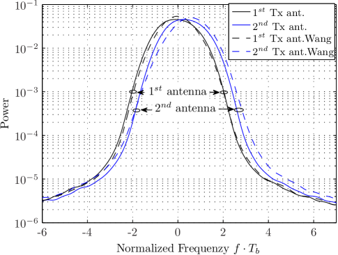
Figure 3: Simulated psd for each Tx antenna of the proposed STC (continuous line) and the Wang-Xia-STC (dashed line)

From the simulation results given in Figure 2, we can reasonably assume that the proposed code achieves full diversity. Indeed, the curves for the 2x1 and 2x2 systems respectively show a slope of 2 and 4. Moreover, the curve of the 2x1 systems follows the same slope as the ST code proposed by Wang and Xia [8], which was proved to have full diversity. Note also that the new code provides a slightly better performance.

A main reason of using CPM for STC is the spectral efficiency. Figure 3 show the simulated power spectral density (psd) for both Tx antennas of the proposed ST code (continuous line) and the ST code proposed by Wang and Xia [8]. The first antenna of our approach uses a conventional CPM signal and hence shows an equal psd. The spectrum of the second antenna is shifted due to adding an offset $c_{mr}(t)$ with a non zero mean. Minimizing the difference between the two spectra by shifting one, result in a phase difference of $0.375$ measured in normalized frequency $f\cdot T_{d}$, where $T_{d}=T/\log_{2}(M)$ is the bit symbol length. The first antenna of the Wang-Xia-algorithm has almost the same psd while the spectrum of the second antenna is shifted by approximately $0.56f\cdot T_{d}$. This means that the OSTC by Wang and Xia requires a slightly larger bandwidth than our OSTC.

V Conclusion

In applications where the power efficiency is crucial, combination of Continuous Phase Modulation and Space Time Coding has the potential to provide high spectral efficiency, thanks to spatial diversity. To address this power efficiency, ST code design for CPM has to ensure both low complexity decoding and full diversity. To fulfill these requirements, we have proposed a new $L^{2}$ orthogonality condition. We have shown that this condition is sufficient to achieve low complexity ML decoding and leads, with the help of simplifying assumption to a simple code. Moreover, simulations indicate that the code most probably achieves full diversity. Further work will be concentrated on the design of other codes based on $L^{2}$ orthogonality as in the meanwhile, we have been able to obtain the design of full diversity, full rate $L^{2}$ orthogonal codes for 3 antennas [10].

References

• [1] S.Β M. Alamouti, β€œA simple transmit diversity technique for wireless communications,” IEEE J. Sel. Areas Commun., vol. 16, no. 8, pp. 1451 – 1458, 1998.
• [2] V.Β Tarokh, H.Β Jafarkhani, and A.Β R. Calderbank, β€œSpace-time block codes from orthogonal designs,” IEEE Trans. Inf. Theory, vol. 45, no. 5, pp. 1456 – 1567, 1999.
• [3] X.Β Zhang and M.Β P. Fitz, β€œSpace-time coding for rayleigh fading channels in CPM system,” Proc. 38th Annu. Allerton Conf. Communication, Control, and Computing, 2000.
• [4] X.Β Zhang and M.Β P. Fitz, β€œSpace-time code design with continuous phase modulation,” IEEE J. Sel. Areas Commun., vol. 21, no. 5, pp. 783 – 792, 2003.
• [5] A.Β ZajiΔ‡ and G.Β StΓΌber, β€œA space-time code design for partial-response CPM: Diversity order and coding gain,” IEEE ICC, 2007.
• [6] A.-M. Silvester, L.Β Lampe, and R.Β Schober, β€œDiagonal space-time code design for continuous-phase modulation,” GLOBECOM, 2006.
• [7] G.Β Wang and X.-G. Xia, β€œAn orthogonal space-time coded CPM system with fast decoding for two transmit antennas,” IEEE Trans. Inf. Theory, vol. 50, no. 3, pp. 486 – 493, 2004.
• [8] D.Β Wang, G.Β Wang, and X.-G. Xia, β€œAn orthogonal space-time coded partial response CPM system with fast decoding for two transmit antennas,” IEEE Trans. Wireless Commun., vol. 4, no. 5, pp. 2410 – 2422, 2005.
• [9] J.B. Anderson, T.Β Aulin, and C.-E. Sundberg, Digital Phase Modulation, Plenum Press, 1986.
• [10] M.Β Hesse, J.Β Lebrun, and L.Β Deneire, β€œL2 OSTC-CPM: Theory and design,” Tech. Rep. I3S/RR-2008-03, CNRS/University of Nice, Sophia Antipolis, 2008.