Three Dimensional Lattice-Boltzmann Model for Electrodynamics

Abstract

In this paper we introduce a novel 3D Lattice-Boltzmann model that recovers in the continuous limit the Maxwell equations in materials. In order to build conservation equations with antisymmetric tensors, like the Faraday law, the model assigns four auxiliary vectors to each velocity vector. These auxiliary vectors, when combined with the distribution functions, give the electromagnetic fields. The evolution is driven by the usual BGK collision rule, but with a different form for the equilibrium distribution functions. This LBGK model allows us to consider for both dielectrics and conductors with realistic parameters, and therefore it is adequate to simulate the most diverse electromagnetic problems, like the propagation of electromagnetic waves (both in dielectric media and in waveguides), the skin effect, the radiation pattern of a small dipole antenna and the natural frequencies of a resonant cavity, all with 2% accuracy. Actually, it shows to be one order of magnitude faster than the original FDTD formulation by Yee to reach the same accuracy. It is, therefore, a valuable alternative to simulate electromagnetic fields and opens lattice Boltzmann for a broad spectrum of new applications in electrodynamics.

I Introduction

The simulation of electromagnetic fields inside materials is a fundamental tool in optics and electrodynamics, even more when boundary conditions and geometries are so complex that an analytical solution is out of question. Some examples are the design of antennas and the study of electrical discharges across inhomogeneous media. For this purpose, several numerical methods have been implemented. A typical and well known example is the FDTD (Finite-difference time-domain) method, which solves the time-dependent Maxwell equations through a finite differences scheme proposed by Yee Yee (1966); Taflove and Hagness (2000); Kunz and Luebbers (1993). The method works pretty well in a broad range of applications, but its stability strongly depends on the mesh size and the time step. Several alternatives have been introduced, e. g. the Chebyshev Raedt et al. (2008) and the unconditionally stable FDTD Zheng et al. (2000), just to name a few.

In the last two decades, the arrival of Lattice Boltzmann methods has been used as an alternative for the simulation of partial differential equations. Originally motivated as discrete realizations of kinetic models for fluids McNamara and Zanetti (1988); Higuera et al. (1989), they have also been developed for the simulation of diffusion Flekkoy (1993), waves Chopard and Droz (1998); Chopard et al. (1997) and even quantum mechanics Succi (2002a, b); Succi and Benzi (1993) and relativistic hydrodynamics Mendoza et al. (2010). Electromagnetic fields, in contrast, have been introduced meanwhile by models for plasmas, mostly in the form of magnetic diffusion equations in resistive magnetohydrodynamics (MHD).

The first two-dimensional LB model reproducing the resistive MHD equations was developed by S. Succi et. al. Succi et al. (1991). Here, the authors showed how a LB for the Navier-Stokes equations could be extended to include two-dimensional magnetic fields and made systematic studies in order to investigate the efficiency in terms of computational time. Later on, other LB models have come as alternativesChen et al. (1991); Martinez et al. (1994); Osborn (2004). S. Chen et al. Chen et al. (1991) studied linear and nonlinear phenomena using a LB model and showed that their method is competitive with traditional solution methods. In another work by D.O. Martinez et al. Martinez et al. (1994), a new LB model for resistive magnetohydrodynamics was proposed where the number of moving vectors could be reduced from $37$ (used in previous works) to $13$, dramatically decreasing the amount of computational memory requested. One of the first models for magnetohydrodynamics in 3D was developed by Osborn Osborn (2004), where he used $19$ vectors on a cubic lattice for the fluid, plus $7$ vectors for the magnetic field, which makes a total number of $26$ vectors per cell. Subsequently, Fogaccia, Benzi and Romanelli Fogaccia et al. (1996) introduced a 3D LB model for turbulent plasmas incorporating the electric potential in the electrostatic limit. Among the many works on LBM for MHD, the one proposed by Paul Dellar Dellar (2002) deserves a special attention for the present work. It introduces the curl of the electric field (i.e. the divergence of an antisymmetric tensor) indirectly, by using a vector-valued distribution for the magnetic field which obeys a vector Boltzmann BGK equation Bouchut (1999), and is only coupled with the fluid distribution function via the macroscopic variables evaluated at the lattice points.

In a recent workMendoza and Munoz (2008a), the authors introduced a 3D LB model that reproduces the two-fluids theory for plasmas. The model employs 39 independent vectors (including both D3Q19 velocity vectors for the fluids, D3Q13 auxiliary vectors for the electric field and D3Q7 auxiliary vectors for the magnetic one) and uses in general four density distribution functions per velocity vector: one for the electrons, one for the ions and two for the electromagnetic fields in vacuum. The curls associated with the Faraday and Ampére laws in vacuum are explicitly constructed by means of the auxiliary vectors mentioned above. The model reproduces the Hartman flow and allows to reconstruct the phenomenon of magnetic reconnection in the magnetotail with the true mass ratio between electrons and ions. However, the problem of reproducing the Maxwell equations in media is not addressed in that work. The solution requires for doubling the distribution functions dealing with the electromagnetic fields, as we will show in the present manuscript, plus additional forcing terms to account for the sources. Once the terms related with the plasma fields (electrons and ions) are removed, the set of velocity vectors can be simplified to D3Q13, because we do not have viscous terms (the relaxation time is $\tau$$=$$1/2$ and the procedure is still stable as a consequence of the linear nature of Maxwell equations). The result is a complete model that successfully reproduces the behavior of electromagnetic fields inside dielectrics, magnets and conductors and gathers information about the current density, electric charge, and electromagnetic fields everywhere. The model is second-order accuracy in time and performs well in a wide range of traditional benchmarks, with errors below 1% in the fields.

Section II describes the model, with the evolution rules and the equilibrium expressions for the 50 density functions, plus the procedure to compute for the charge and current densities and the electric and magnetic fields. This section also reviews how the auxiliary vectors and the equilibrium distributions achieve the construction of the curls in the Maxwell equations. The Chapman-Enskog expansion showing how these rules recover the electrodynamic equations with second-order accuracy is developed in Appendix A. In order to validate the model, we simulate in section III the reflection of an electromagnetic pulse on the frontier between two dielectric media, the propagation of electromagnetic waves along a microstrip waveguide, the skin effect inside a conductor, the radiation pattern of an oscillating electrical dipole (including a comparison between LB and Yee) and the resonant responses of a cubic cavity. The main results and conclusions are summarized in section IV.

II 3D Lattice-Boltzmann Model for Electrodynamics

In a simple Lattice-Boltzmann model McNamara and Zanetti (1988) the $D$-dimensional space is divided into a regular grid of cells. Each cell has $Q$ vectors $\vec{v}_{i}$ linking with the neighboring cells, and each vector has associated a distribution function $f_{i}$. This distribution function evolves according to the Boltzmann equation,

$${}f_{i}(\vec{x}+\vec{v}_{i},t+1)-f_{i}(\vec{x},t)=\Omega_{i}(\vec{x},t)\quad,$$ (1)

where $\Omega_{i}(\vec{x},t)$ is a collision term, usually taken as a time relaxation to some equilibrium function, $f_{i}^{\rm eq}$. This is known as the Bhatnagar-Gross-Krook (BGK) operator Bathnagar et al. (1954),

$${}\Omega_{i}(\vec{x},t)=-\frac{1}{\tau}(f_{i}(\vec{x},t)-f_{i}^{\rm eq}(\vec{x},t))\quad,$$ (2)

where $\tau$ is the relaxation time. The equilibrium function is chosen in such a way, that (in the continuum limit) the model simulates the actual physics of the system.

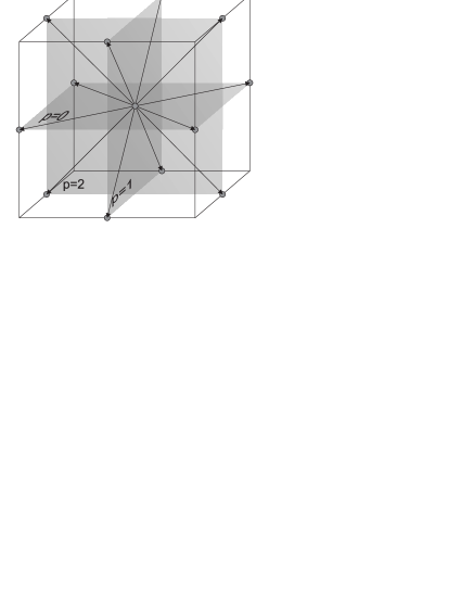
Figure 1: Cubic cell D3Q13 to model the Maxwell equations. The arrows represent the velocity vectors $\vec{v}_{i}^{p}$ and the electric field vectors $\vec{e}_{ij}^{p}$, where $p$ indicates the plane of location.

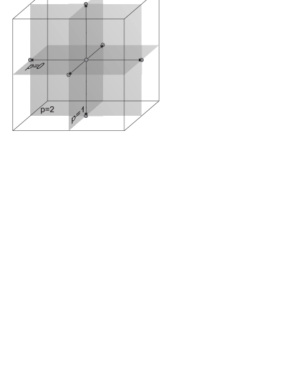
Figure 2: Cubic cell D3Q7 to simulate the magnetic field. The arrows indicate the magnetic vectors $\vec{b}_{ij}^{p}$.

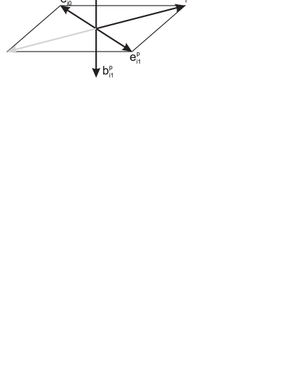
Figure 3: Index relationship between the velocity vectors and the electric and magnetic vectors.

In our case, we need to reproduce the Maxwell equations in materials. Two of them are the Faraday’s law,

$${}\frac{\partial\vec{B}}{\partial t}+\vec{\nabla}\times\vec{E}=0\quad,$$ (3)

and the Ampère’s law,

$${}\frac{\partial\vec{D}}{\partial t}-c^{2}\vec{\nabla}\times\vec{H}+\mu_{0}\vec{J}=0\quad,$$ (4)

where $\vec{B}$ is the induction field, $\vec{E}$ is the electric field, $\vec{D}$ is the displacement field and $\vec{J}$ is the current density. These are conservation equations including curls, which can be written in tensorial form as

$${}\frac{\partial\vec{B}}{\partial t}+\vec{\nabla}\cdot\Lambda=0$$ (5)

for the Faraday’s law, and

$${}\frac{\partial\vec{D}}{\partial t}+\vec{\nabla}\cdot\Gamma+\mu_{0}\vec{J}=0$$ (6)

for the Ampère’s law, with the antisymmetric tensors

$$\Lambda=\left(\begin{array}[]{ccc}0&-E_{z}&E_{y}\\ E_{z}&0&-E_{x}\\ -E_{y}&E_{x}&0\end{array}\right)$$ (10)

and

$$\Gamma=\left(\begin{array}[]{ccc}0&c^{2}B_{z}&-c^{2}B_{y}\\ -c^{2}B_{z}&0&c^{2}B_{x}\\ c^{2}B_{y}&-c^{2}B_{x}&0\end{array}\right)\quad.$$ (14)

Let us choose a cubic regular grid of lattice constant $\delta x$$=$$\sqrt{2}c\delta t$, with $c$ the light speed in vacuum ($c$$\simeq$$3\times 10^{8}m/s$); that is, $c$$=$$1/\sqrt{2}$ in normalized lattice units (time unit $=$$\delta t$, spatial unit $=$$\delta x$), and the Courant-Fredericks-Levy criterion is automatically fulfilled. There are $13$ velocity vectors per cell (figure 1), plus 13 different vectors for the electric field (figure 1) and 7 different vectors for the magnetic field (figure 2). The velocity vectors are denoted by $\vec{v}_{i}^{p}$, where $i$$=$$1,2,3,4$ indicates the direction and $p$$=$$0,1,2$ indexes the plane of location (Fig. 1). They have magnitude $\sqrt{2}$ (in lattice units) and lie on the diagonals of the planes. In components,

$$\vec{v}_{i}^{0}=\sqrt{2}(\cos((2i-1)\pi/4),\sin((2i-1)\pi/4),0)\quad,$$ (15a)

$$\vec{v}_{i}^{1}=\sqrt{2}(\cos((2i-1)\pi/4),0,\sin((2i-1)\pi/4))\quad,$$ (15b)

$$\vec{v}_{i}^{2}=\sqrt{2}(0,\cos((2i-1)\pi/4),\sin((2i-1)\pi/4))\quad,$$ (15c)

They, plus the rest vector $\vec{v}_{0}$$=$$(0,0,0)$, give us $13$ vectors. It is well known that the configuration D3Q13 has problems to reproduce for fluids the local momentum conservation during collision, due to a slackness in symmetry. Nevertheless, because we are using $\tau$$=$$\frac{1}{2}$, there are not viscous terms like in the fluid case, and D3Q13 can handle the symmetries we need for the Maxwell equations, as shown below.

Associated to each velocity vector $\vec{v}_{i}^{p}$ there are two electric $\vec{e}_{ij}^{p}$ and two magnetic auxiliary vectors $\vec{b}_{ij}^{p}$ ($j$$=$$0,1$), as shown in Fig.3. They are used to compute the electromagnetic fields. The electric vectors are perpendicular to $\vec{v}_{i}^{p}$ and lie on the same plane $p$. The magnetic vectors are also perpendicular to $\vec{v}_{i}^{p}$, but lying perpendicular to the plane $p$. They are given by

$$\begin{aligned} \vec{e}_{i0}^{p}=\frac{1}{2}\vec{v}_{[(i+2)\mod 4]+1}^{p}&\quad,\quad\vec{e}_{i1}^{p}=\frac{1}{2}\vec{v}_{[i\mod 4]+1}^{p}\quad,\\ \vec{b}_{ij}^{p}&=\vec{v}_{i}^{p}\times\vec{e}_{ij}^{p}\quad.\end{aligned}$$ (16)

The picture is completed by the null vectors $\vec{e}_{0}$$=$$(0,0,0)$ and $\vec{b}_{0}$$=$$(0,0,0)$. With these definitions, there are $25$ electric field vectors, but only $13$ of them are different. Similarly, there are $25$ magnetic field vectors, but only $7$ are different. These vectors satisfy the following properties:

$$\sum_{i,p}\;v_{i\alpha}^{p}=0\quad,$$ (17a)

$$\sum_{i,j,p}\;e_{ij\alpha}^{p}=0\quad,$$ (17b)

$$\sum_{i,j,p}\;v_{i\alpha}^{p}e_{ij\beta}^{p}=0\quad,$$ (17c)

$$\sum_{i,j,p}\;e_{ij\alpha}^{p}e_{ij\beta}^{p}=4\delta_{\alpha\beta}\quad,$$ (17d)

$$\sum_{i,j,p}\;v_{i\alpha}^{p}e_{ij\beta}^{p}e_{ij\gamma}^{p}=0\quad,$$ (17e)

$$\sum_{i,j,p}\;v_{i\alpha}^{p}e_{ij\beta}^{p}b_{ij\gamma}^{p}=4\epsilon_{\alpha\beta\gamma}\quad,$$ (17f)

$$\sum_{i,j,p}\;b_{ij\alpha}^{p}b_{ij\beta}^{p}=8\delta_{\alpha\beta}\quad,$$ (17g)

where $\epsilon_{\alpha\beta\gamma}$ are the components of the Levi-Civita tensor, defined as usual: If two indexes are equal, the component is zero, $\epsilon_{123}$$=$$1$ and any odd permutation of indexes changes the component sign. The property (17f) is indeed the one that allow us to construct conservation laws with antisymmetric tensors, as we will show below.

The electromagnetic fields are computed from distribution functions propagating from cell to cell with the velocity vectors $\vec{v}_{i}^{p}$. There are four distribution functions associated with each non-zero velocity vector, denoted by $f_{ij}^{p(r)}$ ($j$$=$$0,1$ and $r$$=$$0,1$), plus two functions associated with the rest vector $\vec{v}_{0}$, denoted by $f_{0}^{(r)}$. This makes $4\times 12+2$$=$$50$ distribution functions.The macroscopic fields are computed as follows:

$$\vec{D}=\sum_{i=1}^{4}\sum_{p=0}^{2}\sum_{j=0}^{1}f_{ij}^{p(0)}\vec{e}_{ij}^{p}\quad,$$ (18a)

$$\vec{B}=\sum_{i=1}^{4}\sum_{p=0}^{2}\sum_{j=0}^{1}f_{ij}^{p(1)}\vec{b}_{ij}^{p}\quad,$$ (18b)

$$\rho_{c}=f_{0}^{(0)}+\sum_{i=1}^{4}\sum_{p=0}^{2}\sum_{j=0}^{1}f_{ij}^{p(0)}\quad,$$ (18c)

$$\vec{E}=\frac{\vec{D}}{\epsilon_{r}}\quad,$$ (18d)

$$\vec{H}=\frac{\vec{B}}{\mu_{r}}\quad,$$ (18e)

$$\vec{J}=\sigma\vec{E}\quad,$$ (18f)

where $\vec{D}$, $\vec{E}$ and $\vec{J}$ are subsidiary fields representing the displacement field, the electric field and the total current density before external forcing, respectively (the actual mean fields, including external forcing, are described below). In addition, $\vec{B}$ is the induction field, $\vec{H}$ is the magnetic field, $\rho_{c}$ is the total charge density and $\epsilon_{r}$, $\mu_{r}$ and $\sigma$ are the relative dielectric constant, the relative permeability constant and the conductivity for the medium, respectively. Notice that we define $\vec{D}$ and $\vec{H}$ just with the relative constants $\epsilon_{r}$ and $\mu_{r}$, instead of the total electromagnetic constants $\epsilon$$=$$\epsilon_{r}\epsilon_{0}$ and $\mu$$=$$\mu_{r}\mu_{0}$.

The velocity vectors $\vec{v}_{i}^{p}$ are not mean to represent the velocity of any particles (in contrast with the normal lattice Boltzmann models for fluids), because in classical electrodynamics there are not such particles, but they can be related with Poynting vectors describing the momentum density flux of the electromagnetic fields. This interpretation can be supported by looking at Eqs. 18 and Fig. 3, and recognizing on the figure the implicit cross product that defines the Poynting vector as $\vec{S}$$=$$\frac{1}{\mu_{r}\epsilon_{r}}\vec{D}\times\vec{B}$David (1966).

For the collision we adopt terms $\Omega_{ij}^{p(r)}$ and $\Omega_{0}^{(r)}$ of the BGK form Bathnagar et al. (1954)

$$\Omega_{ij}^{p(r)}=-\frac{1}{\tau}(f_{ij}^{p(r)}(\vec{x},t)-f_{ij}^{p(r)\rm eq}(\vec{x},t))\quad,$$ (19a)

$$\Omega_{0}^{(r)}=-\frac{1}{\tau}(f_{0}^{(r)}(\vec{x},t)-f_{0}^{(r)\rm eq}(\vec{x},t))\quad.$$ (19b)

where the relaxation time is chosen $\tau$$=$$\frac{1}{2}$. Since Maxwell equations are linear, this relaxation time does not produce any instability.

In order to include the source term in the Ampere’s law (4), we need of external forcing terms. These terms are included by following the proposal of Zhaoli Guo, Chuguang Zheng and Baochang Shi Guo et al. (2002), as follows:

$${}\begin{aligned} f_{ij}^{p(r)}(\vec{x}+\vec{v}_{i}^{p},t+1)-f_{ij}^{p(r)}(\vec{x},t)=&\Omega_{ij}^{p(r)}(\vec{x},t)+T_{ij}^{p(r)},\end{aligned}$$ (20)

$${}f_{0}^{(r)}(\vec{x},t+1)-f_{0}^{(r)}(\vec{x},t)=\Omega_{0}^{(r)}(\vec{x},t)+T_{0}^{(r)}\quad,$$ (21)

where $T_{ij}^{(r)}$ and $T_{0}^{(r)}$ are forcing coefficients ($r$$=$$0,1$). These coefficients are defined by Guo et al. (2002)

$$\begin{aligned} T_{ij}^{p(r)}&=\biggl{(}1-\frac{1}{2\tau}\biggr{)}\biggl{(}\frac{1}{4}(\vec{e}_{ij}^{p}-\vec{E^{\prime}})\cdot\vec{F}\\ &+\frac{3}{4}(\vec{e}_{ij}^{p}\cdot\vec{E^{\prime}})(\vec{e}_{ij}^{p}\cdot\vec{F})\biggr{)}\quad,\end{aligned}$$ (22a)

$$T_{0}^{(r)}=\biggl{(}1-\frac{1}{2\tau}\biggr{)}\biggl{(}-\frac{1}{4}(\vec{E^{\prime}})\cdot\vec{F}\biggr{)}\quad,$$ (22b)

with $\vec{F}$ the external forcing. Since $\tau$$=$$1/2$, $T_{ij}^{p(r)}$$=$$T_{0}^{(r)}$$=$$0$, and the forcing only appears in the mean fields. The mean electric field, $\vec{E^{\prime}}$, and the mean density current vector, $\vec{J^{\prime}}$, are given by

$$\vec{E^{\prime}} = \vec{E}-\frac{\mu_{0}}{4\epsilon_{r}}\vec{J^{\prime}}\quad,{}$$ (23)

$$\vec{J^{\prime}} = \sigma\vec{E^{\prime}}\quad.{}$$ (24)

Replacing Eq.(23) into Eq.(24) gives us the mean density vector $\vec{J^{\prime}}$ in terms of the subsidiary fields,

$${}\vec{J^{\prime}}=\frac{\sigma}{1+\frac{\mu_{0}\sigma}{4\epsilon_{r}}}\vec{E}\quad.$$ (25)

Finally, the equilibrium distribution functions for the electromagnetic fields are given by

$$f_{ij}^{p(0)\rm eq}(\vec{x},t)=\frac{1}{16}\vec{v}_{i}^{p}\cdot\vec{J^{\prime}}+\frac{\epsilon}{4}\vec{E^{\prime}}\cdot\vec{e}_{ij}^{p}+\frac{1}{8\mu}\vec{B}\cdot\vec{b}_{ij}^{p}\quad,$$ (26a)

$$f_{ij}^{p(1)\rm eq}(\vec{x},t)=\frac{1}{16}\vec{v}_{i}^{p}\cdot\vec{J^{\prime}}+\frac{1}{4}\vec{E^{\prime}}\cdot\vec{e}_{ij}^{p}+\frac{1}{8}\vec{B}\cdot\vec{b}_{ij}^{p}\quad,$$ (26b)

$$f_{0}^{(0)\rm eq}(\vec{x},t)=f_{0}^{(1)\rm eq}(\vec{x},t)=\rho_{c}\quad,$$ (26c)

where the two sets ($r$$=$$0,1$) of equilibrium density functions ($f_{ij}^{p(r)\rm eq}$) are made explicit. This structure for the equilibrium functions allows for the construction of conservative laws with curls. Indeed, performing the Chapman-Enskog expansion of the BGK evolution equation with these equilibrium functions, but multiplying by $\vec{b}_{ij}^{p}$ – instead of the traditional multiplication by the velocity vectors $\vec{v}_{i}^{p}$ (see Appendix A) – before summing up over the index $i$, $j$ and $p$, we obtain the time derivative of the magnetic field equals to the divergence of the antisymmetric tensor (14). The tensor becomes antisymmetric because this procedure builds up the Levi-Civita tensor, as follows: The Chapman-Enskog expansion gives a velocity vector $\vec{v}_{i}^{p}$, the equilibrium function contributes with a vector $\vec{e}_{ij}^{p}$ and multiplying by $\vec{b}_{ij}^{p}$ and summing up over $i$, $j$ and $p$ gives us $\epsilon_{\alpha\beta\gamma}E^{\prime}_{\gamma}$ for the tensor (Eq. 17f), that is the Faraday’s law. Ampère’s law is obtained by multiplying by $\vec{e}_{ij}^{p}$ (instead of $\vec{b}_{ij}^{p}$) and following the same procedure. This completes the definition of the lattice Boltzmann model. The detailed proof that this LBGK model, via a Chapman-Enskog expansion, recovers the Maxwell equations is shown in Appendix A.

The model reproduces the following equations:

$$\frac{\partial\rho_{c}}{\partial t}+\nabla\cdot\vec{J^{\prime}}=0\quad,$$ (27a)

$$\nabla\times\vec{E^{\prime}}=-\frac{\partial\vec{B}}{\partial t}\quad,$$ (27b)

$$\nabla\times\vec{H}=\mu_{0}\vec{J^{\prime}}+\frac{1}{c^{2}}\frac{\partial\vec{D^{\prime}}}{\partial t}\quad.$$ (27c)

It is well known David (1966) that these three conservative laws implies the following expressions for the divergence of the electromagnetic fields:

$$\frac{\partial}{\partial t}\left(\nabla\cdot\vec{D^{\prime}}-\frac{\rho_{c}}{\epsilon_{0}}\right)=0\quad,$$ (28a)

$$\frac{\partial}{\partial t}\left(\nabla\cdot\vec{B}\right)=0\quad;$$ (28b)

that is, the other two Maxwell equations are reproduced if they are satisfied by the initial condition (for more details see Appendix A).

III Numerical Tests

In order to validate our model, we have implemented several tests. Let us start with two simple simulations showing that the model reproduces the correct electromagnetic propagation with dielectrics and conductors. We will construct more complex simulations afterward, like the radiation pattern from an oscillating electric dipole, the wave propagation on a waveguide, and the identification of the normal modes in a cubic resonance cavity. Additionally, in this section, we compare the results obtained by using LB and Yee methods for the case of the radiation produced by an oscillating dipole.

III.1 Dielectric Interface

As a first benchmark let us simulate the propagation of an electromagnetic Gaussian pulse crossing a dielectric interface. For this purpose, we took an uni-dimensional array of $L$ cells with periodic boundary conditions in the $z$ coordinate and with each cell being its own neighbor in both $x$ and $y$ directions. One half of the simulation space, $z$$<$$L/2$, is vacuum ($\epsilon$$=$$\epsilon_{0}$) and the other half, $z$$>$$L/2$, represents a dielectric medium with relative dielectric constant $\epsilon_{r}$$=$$\epsilon/\epsilon_{0}$$=$$2.5$. In order to avoid for abrupt changes on the dielectric constant between two neighboring cells we choose the following distribution of the permittivity:

$$\epsilon_{\rm r}=1.75+0.75\tanh(x-L/2)\quad.$$ (29)

The functional form of the incident Gaussian electromagnetic pulse centered at $z_{0}$ is given by

$$\vec{E}=(E_{0}\exp(-\alpha(z-z_{0})^{2}),0,0)\quad,$$ (30a)

$$\vec{B}=(0,B_{0}\exp(-\alpha(z-z_{0})^{2}),0)\quad.$$ (30b)

The constant $\alpha$ fixes the pulse width, $E_{0}$ is the pulse amplitude and the constant $B_{0}$ is related with $E_{0}$ according to the relation $E_{0}$$=$$cB_{0}$, with $c$ the vacuum light speed. For the simulation we choose $L$$=$$200$, $c$$=$$1/\sqrt{2}$, $E_{0}$$=$$0.001$, $\alpha$$=$$0.01$ y $z_{0}$$=$$40$ (in normalized units). The initial condition and the electric field after $140$ time steps is shown in figure 4.

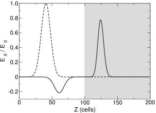
Figure 4: Electric pulse crossing a dielectric interface. The shadow zone is the dielectric medium, with dielectric constant $\epsilon_{r}$$=$$2.5$ and the other one corresponds to the vacuum ($\epsilon_{r}$$=$$1.0$). The curves are the intensity of the electric field at $t$$=$$0$ (dashed line), and at $t$$=$$140$ (solid line).

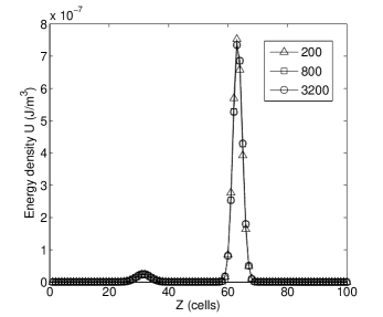
Figure 5: Energy density $U$ as a function $z$ at $t$$=$$140$ for an electric pulse crossing a dielectric interface for different grid resolutions: $200$, $800$, and $3200$ cells.

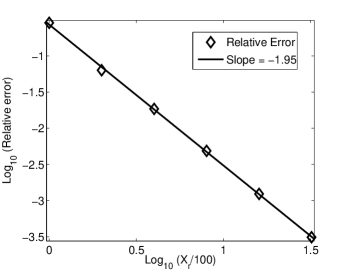
Figure 6: Total relative error $E_{T}$ of the energy density $U$ as a function of the grid size for an electric pulse crossing a dielectric interface. Here $X_{r}$ is the number of grid points, and the error is computed by $E_{T}$$=$$\frac{1}{L}\sum_{i=1}^{L}E_{r}$, with $L$ the grid size and $E_{r}$ the error at each cell location given by Eq. (34).

The theoretical predictions for the amplitudes of the transmitted and reflected pulses can be computed from David (1966)

$$\frac{E_{0}^{\prime}}{E_{0}}=\frac{2}{\sqrt{\frac{\epsilon_{r}^{\prime}}{\epsilon_{r}}}+1}\quad,$$ (31a)

$$\frac{E_{0}^{\prime\prime}}{E_{0}}=\frac{\sqrt{\frac{\epsilon_{r}^{\prime}}{\epsilon_{r}}}-1}{\sqrt{\frac{\epsilon_{r}^{\prime}}{\epsilon_{r}}}+1}\quad.$$ (31b)

They give us $\frac{E_{0}^{\prime}}{E_{0}}$$=$$0.7751$ and $\frac{E_{0}^{\prime\prime}}{E_{0}}$$=$$0.2249$. The values from the simulation are $0.7750$ and $0.2249$, respectively, that is the errors are smaller than $1\%$. This simulation takes less than 30 ms in a standard PC.

Because we are dealing with conservative equations in the differential form, we need to calculate the order of convergence of the model. Let us track how does it change the accuracy of a physical variable when the resolution of the spatial grid $\delta x$ increases. The time resolution increases in the same way, because $\delta x=\sqrt{2}c\delta t$, with $c$ the speed of light. We choose to track the electromagnetic energy density $U$, defined by

$$U=\frac{1}{2}\left(\epsilon_{r}\vec{E}\cdot\vec{E}+\frac{1}{\mu_{r}}\vec{B}\cdot\vec{B}\right)\quad.$$ (32)

Fig. 5 shows the electromagnetic energy density $U$ as a function of the $z$-coordinate for different grid sizes ($200$, $800$ and $3200$ grid points). We use Richardson’s method Richardson (1911); Richardson and Gaunt (1927) to compute the convergence error for the model. First, let us estimate the exact solution of $U$ up to order $n$ by using the expression

$$U=\lim_{\delta x\rightarrow 0}U(\delta x)\approx\frac{2^{n}U\left(\frac{\delta x}{2}\right)-U(\delta x)}{2^{n}-1}+\vartheta(\delta x^{n+1})\quad,$$ (33)

with errors $\vartheta(\delta x^{n+1})$ of order $n+1$. Here, we set $n=2$. Thus, the relative error at each cell between the value $U(\delta x)$ and the “exact” solution $U$ is computed by

$$E_{r}(\delta x)=\left|\frac{U(\delta x)-U}{U}\right|\quad.$$ (34)

The total relative error $E_{T}$ is computed just by adding the errors $E_{r}$ on all cells. Fig. 6 shows that this error decreases as $\delta x^{1.95}$, supporting that the present scheme has a second-order convergence, i. e. the convergence behavior we expected for our LB model.

III.2 Skin Effect

The skin effect is the exponential decay in the amplitude of a plane wave penetrating a conducting medium. To reproduce the effect we construct an uni-dimensional space of $L$ cells as before, with zero conductivity for $z$$<$$L/4$ and $\sigma_{0}$ conductivity for $z$$>$$L/4$. We choose an smooth conductivity transition of the form

$$\sigma=\sigma_{0}(1+\tanh(x-L/4))\quad,$$ (35)

to avoid numerical instabilities. The incoming plane wave is generated by imposing a harmonic oscillation of the electric field at $z$$=$$0$,

$$\vec{E}=(E_{0}\sin(\omega t),0,0)\quad,$$ (36a)

$$\vec{B}=(0,B_{0}\sin(\omega t),0)\quad,$$ (36b)

where $E_{0}$ is the wave amplitude, $B_{0}$$=$$E_{0}/c$ and $\omega$ is the angular frequency.

Figure 7: Numerical reproduction of the skin effect. A plane wave impacts perpendicular a conducting medium at $z$$=$$250$. The dashed, dot and dot-dashed lines draw the electric field inside the conductor as a function of depth after $635$, $647$ and $670$ time steps, respectively. The solid line is the theoretical exponential decrease one expects for the amplitude of the incident wave. One can observe that the first maxima of the incident waves lie on the expected exponential curve.

The simulation is shown in Figure 7, with $L$$=$$1000$, $E_{0}$$=$$0.001$, $\omega$$=$$\pi/100$, $c$$=$$1/\sqrt{2}$ and $\sigma_{0}$$=$$10^{6}$ (in normalized units). The theoretical expression for the amplitude of the oscillating electric field inside the conductor is

$$E=E_{0}\exp(-x/\Delta)\quad,$$ (37)

where $E_{0}$ is the amplitude of the electric field just outside and $\Delta$ is known as the skin thickness. For good conductors this thickness is given by David (1966)

$$\Delta=\sqrt{\frac{2}{\sigma\mu\omega}}\quad.$$ (38)

Figure 7 also shows the analytical solution given by Eq. (37) as a solid line. One can observe that the amplitude of the electric field oscillation follows in excellent agreement the theoretical prediction. This simulation took less than 30 ms in a single Pentium IV at 3.0 GHz.

III.3 Electric Dipole

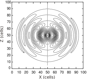
Figure 8: Lines of equal intensity of the magnetic field produced by an oscillating electric dipole in $z$ after two whole oscillations (approximately).

In order to simulate the radiation pattern of a small electric dipole antenna we construct an array of $L\times L\times L$, with $L$$=$$100$ cells with free boundary conditions (each limit cell takes itself as his own missing neighbor). In the center of this array we insert a small oscillating current density in the $z$ direction,

$$J_{z}=J^{\prime}_{0}\sin\biggr{(}\frac{2\pi}{T}t\biggl{)}\quad,$$ (39)

where $J^{\prime}_{0}$ is the amplitude of the current density and $T$ is the oscillation period. For avoiding any abrupt change of the physical quantities between two neighboring cells we choose actually a Gaussian functional form for the amplitude of the current density $J^{\prime}_{0}$,

$$J^{\prime}_{0}=J_{0}\exp(-0.75[(x-50)^{2}+(y-50)^{2}+(z-50)^{2}])\quad.$$ (40)

The period was set to $T$$=$$25.0$ time steps and the amplitude to $J_{0}$$=$$0.0001$ (in automaton units).

The results are shown in Figures 8 and 9. Figure 8 draws the lines of equal intensity of the magnetic field after $56$ time steps. Figure 9 shows the amplitude of the radiated magnetic field along the $x$ axis, compared both with a set of results from Yee simulations for several grid resolutions and with the theoretical values for the peaks, given by David (1966)

$$B=\frac{k^{2}P}{x}\sqrt{1-\frac{1}{k^{2}x^{2}}}\quad.$$ (41)

Here, $k$$=$$\frac{\omega}{c}$ is the magnitude of the wave vector, with $c$ the speed of light in vacuum and $\omega$ the angular frequency. The magnitude $P$ of the electric dipole momentum is computed by

$$P=\frac{J_{0}\Sigma}{\omega}\quad,$$ (42)

where $\Sigma$ is the effective volume for the dipole. The Yee method was implemented for three resolutions: $100\times 100\times 100$, $200\times 200\times 200$, and $300\times 300\times 300$ grid points, in contrast with the array of $100\times 100\times 100$ cells for our LB method. Table 1 shows the amplitude of the peaks computed from the LB and Yee methods and contrasted the theoretical values.

Amp. LB	Amp. Yee	Amp. Yee	Amp. Yee	Theo. value
$L=100$	$L=100$	$L=200$	$L=300$	$B_{theo}$
$B_{sim,LB}$	$B_{sim,Yee}$	$B_{sim,Yee}$	$B_{sim,Yee}$
23.33	21.00	22.18	22.62	23.01
9.53	9.21	9.38	9.38	9.37
6.12	6.05	6.09	6.15	6.07
4.54	4.47	4.56	4.54	4.51

Table 1: Amplitude of the peaks of Fig. 9 computed form our LB model ($B_{sim,LB}$) with a resolution of $L=100$ cells and from the Yee’s method ($B_{sim,Yee}$) with several resolutions. The theoretical values ($B_{theo}$) predicted by Eq. (41) area also included.

Err. LB	Err. Yee	Err. Yee	Err. Yee
($\%$)	($L=100$), ($\%$)	($L=200$), ($\%$)	($L=300$), ($\%$)
1.4	8.7	3.6	1.6
1.7	1.7	0.1	0.1
0.8	0.3	0.3	1.3
0.7	0.9	1.1	0.7

Table 2: Relative errors on the amplitude of the peaks of Table 1 as contrasted with the theoretical predictions.

The simulation using the LB model matches again the theoretical predictions with an accuracy of less than $2\%$ (see Table 2). In contrast, the Yee’s method with the same grid resolution computes the nearest peak to the source (where the boundary effects are less pronounced) with an error of $8.7\%$, far from the LB one. In order to reach the same accuracy that the LB method, we must increase the grid resolution by the Yee’s method up to $L=300$, but at expenses of high computational costs. The simulation using the LB model takes $23$ seconds in a single standard machine, while the Yee’s method takes $5$ seconds with $L=100$, $67$ seconds for $L=200$ and $336$ seconds for $L=300$, that is around $13$ times more CPU time that the LB for the same errors.

Finally, the results obtained in this section illustrate the possibilities of our method to study the radiation by antennas.

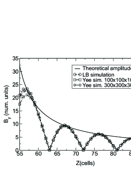
Figure 9: Amplitude along the $x$ axis of the oscillating magnetic field produced by the electric dipole of figure 8. The theoretical envelope corresponds to Eq.(41). The simulation results are obtained by using our LB model with an array of $100\times 100\times 100$ cells (circles) and by the method by Yee with resolutions of $100\times 100\times 100$(squares) and $300\times 300\times 300$ (diamonds) grid points.

III.4 Microstrip Waveguide

Let us simulate the wave propagation on a microstrip waveguide (see figure 11). For this purpose, we chose a 3D array of $100$$\times$$50$$\times$$50$ cells with free boundary conditions and we insert two parallel metallic layers of conductivity $\sigma$, one wider than the other (figure 11), in vacuum.

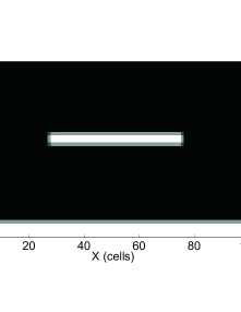
Figure 10: Electric conductivity as a function of $x$ and $z$ at $y$$=$$25$.

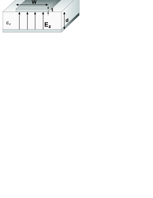
Figure 11: Microstrip waveguide. Here $W$ is the width of the upper metallic plate and $t$ its thickness, $d$ is the dielectric thickness between the two parallel plates with relative permittivity $\epsilon_{r}$ and $E_{z}$ is the electric input signal.

The dimensions, depicted in figure 11, are (in normalized units): $t$$=$$5$, $d$$=$$20$ and $W$$=$$50$. The signal enters into the waveguide by forcing the cells at $y$$=$$0$ to have the electric and magnetic fields of a plane wave (Eqs. (36)) with $E_{0}$$=$$0.01$, $c$$=$$1/\sqrt{2}$ and $\omega$$=$$\pi/100$ (see figure 11). The conductivity is smoothly changed along three cells, as in Sec. III.2 (see figure 10).

Figure 12 shows the $z$ component of the electric field at $y$$=$$25$ after $467$ time steps. The voltage $V(z,t)$ and the current $I(z,t)$ along the waveguide at that time are drawn in figure 13. They are in phase, as expected for a pure traveling wave. The waveguide impedance, computed as $Z_{0}$$=$$V/I$, gives us $Z_{0}$$=$$70.73$ $\Omega$. In contrast, the theoretical value for the impedance of an infinite microstrip waveguide is given by Wheeler (1977)

$$Z=\frac{Z_{0}}{2\pi\sqrt{2(1+\epsilon_{r})}}\ln{\biggl{[}1+\frac{4d}{\omega_{eff}}\biggl{(}\frac{14+\frac{8}{\epsilon_{r}}}{11}\frac{4d}{\omega_{eff}}+\sqrt{\biggl{(}\frac{14+\frac{8}{\epsilon_{r}}}{11}\frac{4d}{\omega_{eff}}\biggr{)}^{2}+\pi^{2}\frac{1+\frac{1}{\epsilon_{r}}}{2}}\biggr{)}\biggr{]}}\quad,$$ (43)

with

$$\omega_{eff}=W+t\frac{1+\frac{1}{\epsilon_{r}}}{2\pi}\ln\Biggl{[}4e\Biggl{(}\biggl{(}\frac{t}{d}\biggr{)}^{2}+\biggl{(}\frac{1}{\pi}\frac{1}{\frac{W}{t}+\frac{11}{10}}\biggr{)}^{2}\Biggr{)}^{-\frac{1}{2}}\Biggr{]}\quad.$$ (44)

From these equations we obtain a theoretical value of $Z_{0}$$=$$72.6$$\Omega$. This gives us a $3$$\%$ difference between the simulation and the theoretical prediction. The simulation takes 83 seconds in a single standard PC.

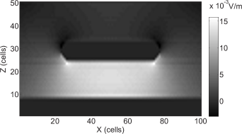
Figure 12: The $z$ component of the electric field in the microstrip at $y$$=$$25$.

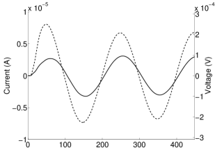
Figure 13: Voltage (dashed line) and current (solid line) in the microstrip waveguide at $y$$=$$25$ as a function of time.

III.5 Resonant Cavity

As a last benchmark, we simulate a cubic resonant cavity and find its resonance frequencies. The cavity is an array of $50$$\times$$50$$\times$$50$ cells, corresponding to a size of $5$$\times$$5$$\times$$5$ $cm$ with periodic boundary conditions, but imposing a null electric field at the boundary (a perfect conductor). An emitter point is set inside the cavity as a single cell with an oscillating electric field in the $x$ direction (the antenna) and a receptor point (the detector) is chosen as a single cell where we measure the electric field amplitude. The emitter point was set at $(5,5,5)$ (in cell units) and the receptor point at $(5,5,45)$. The oscillation frequency was scanned from $0.0182$ to $0.027$ oscillations per time step by multiplying each previous value by a constant factor of $0.0072$, for a total of $22$ different frequencies. Each frequency starts a single run, consisting of $5000$ time steps before equilibrium and four whole oscillations to estimate the amplitude of the electric field.

Figure 14: Frequency spectrum for the resonant cavity with size $50$$\times$$50$$\times$$50$ cells in the frequency range between $0.0182$$clicks^{-1}$ and $0.027$$clicks^{-1}$.

Experimental values	Theoretical values	Error
$\log(f_{exp})$	$\log(f_{the})$	($\%$)
-1.725	-1.724	0.06
-1.690	-1.694	0.24
-1.660	-1.669	0.54
-1.643	-1.646	0.18
-1.618	-1.625	0.43
-1.590	-1.589	0.57

Table 3: Simulational $f_{exp}$ and theoretical $f_{the}$ resonant frequencies for a cavity of size $50$$\times$$50$$\times$$50$ cells. The frequencies are in oscillations per time step.

Figure 14 shows the amplitude of the electric field as a function of frequency. The resonant peaks are clearly identified. Table 3 compares the values for the resonant frequencies with the theoretical predictions computed by David (1966)

$$\omega_{nmp}=\frac{c}{\epsilon_{r}\mu_{r}}\sqrt{\biggl{(}\frac{n\pi}{L_{x}}\biggr{)}^{2}+\biggl{(}\frac{m\pi}{L_{y}}\biggr{)}^{2}+\biggl{(}\frac{p\pi}{L_{z}}\biggr{)}^{2}}\quad.$$ (45)

All differences are smaller than $1\%$. The whole simulation ($22$ runs of more than $5000$ time steps each on a space of $125000$ cells) takes $50$ minutes in a single standard PC.

IV Discussions and Conclusions

In this manuscript, we introduce a three-dimensional LBGK model that reproduces the Maxwell equations in materials. The model successfully accounts for the behavior of electromagnetic fields inside dielectrics, magnets and conductors, and give us information about the current density, electric charge and electromagnetic fields everywhere. It allows us to simulate a broad range of complex phenomena with errors between $1$% and $3$% in all cases we tried, namely: the amplitude of the transmitted and reflected pulses at a dielectric interface, the exponential decay in the amplitude of an incident plane wave inside a conductor (that is, the skin effect), the amplitude (as a function of distance) of the magnetic field radiated by an electric dipole, the characteristic impedance of a microstrip waveguide and the resonant frequencies of a cubic resonant cavity. These five benchmarks prove that our LB model works pretty well in the more different situations.

The model uses D3Q13 velocity vectors, but assigns four auxiliary vectors and four density functions to each one of them. This gives us a total of $33$ vectors and $50$ density functions per cell. These auxiliary vectors allow for the explicit construction of any conservation law with curls, like the Faraday’s and Ampère’s laws Mendoza and Munoz (2008b); a procedure that has also been successful for the construction of a LBGK reproducing the two-fluids model of magnetohydrodynamics Mendoza and Munoz (2008a), but in our case, the density functions dealing with the electromagnetic fields ought to be doubled to account for the Maxwell equations in media. This increase in complexity allows for the more diverse applications, even with realistic values of dielectric, magnetic and conductivity constants.

The equilibrium distribution functions,

$$f_{ij}^{p(r)\rm eq}(\vec{x},t)=\frac{1}{16}\vec{v}_{i}^{p}\cdot\vec{J^{\prime}}+\frac{\epsilon^{1-r}}{4}\vec{E^{\prime}}\cdot\vec{e}_{ij}^{p}+\frac{\mu^{r-1}}{8}\vec{B}\cdot\vec{b}_{ij}^{p}\quad,$$ (46)

with $r$$=$$0,1$, deserve a special discussion. What does these equilibrium function actually mean? If we consider $\vec{e}_{ij}^{p}$ and $\vec{b}_{ij}^{p}$ as small fluctuations in the electromagnetic fields, $\vec{E}$$=$$\vec{E}+\vec{e}_{ij}^{p}$ and $\vec{B}$$=$$\vec{B}+\vec{b}_{ij}^{p}$, the increment in the energy density, at first order, is

$$\Delta U(\vec{E},\vec{B})=\epsilon(\vec{E}\cdot\vec{e}_{ij}^{p})+\frac{1}{\mu}(\vec{B}\cdot\vec{b}_{ij}^{p})\quad,$$ (47)

which resembles our expression for the equilibrium distribution functions $f_{ij}^{p(0)\rm eq}$. So, we argue that such equilibrium functions can be interpreted as changes in the electromagnetic energy density propagating along the velocity vectors $\vec{v}_{i}^{p}$. Moreover, because the auxiliary vectors $\vec{e}_{ij}^{p}$ are related to the electric field and the vectors $\vec{b}_{ij}^{p}$ related to the magnetic field, the velocity vectors $\vec{v}_{i}^{p}$$=$$\vec{e}_{ij}^{p}\times\vec{b}_{ij}^{p}$ can be linked to the direction of the Poynting vector, in some sense.

The model allows us to select the electromagnetic constants (magnetic permeability, electric permittivity and conductivity) for each cell at pleasure. It just needs to smooth the transition between two different materials across three cells, approximately, in order to avoid numerical instabilities (this is the limit of stability), but this is a standard procedure in many numerical models Yee (1966); Whitted (1980). For these reasons, our LB seems to be promising in a variety of applications, including among others: the propagation of electromagnetic pulses inside microcircuits produced by atmospheric rays or discharge antennas, the electromagnetic diffraction across objects with complex geometries or the electromagnetic propagation across meta-materials. They can also be an excellent alternative for the design and optimization of antennas, which requires to simulate a large number of configurations, and very specially in the design of pulse antennas, where single-frequency numerical methods fail. All these applications can be theme of future works.

In terms of speed, our model is one order of magnitude faster than the original Yee’s FDTD methodYee (1966); Taflove and Hagness (2000); Kunz and Luebbers (1993) to obtain the same accuracy level on the simulation of the electromagnetic fields produced by an oscillating electrical dipole. Actually, the grid resolution of the Yee’s method must be increased three times in order to reach the same accuracy than our LB method. It is interesting to discuss why it could be. Yee’s method uses six variables per cell (three for the electric field and three for the magnetic one), but each cell has also to look at the variables of all six first neighbors to evolve in time, gathering a total of $42$ floating point variables to evolve each cell at every time step. For comparison, our LB method uses $50$ floating point variables per cell (the distribution functions), i. e. a similar number of variables to process, but it takes around five times longer to evolve a LB cell than a FDTD cell by the method of Yee. On terms of memory consuming, our LB uses $50$ floating point variables per cell, that is eight times more memory per cell than Yee’s method, but this last requires three times more spatial resolution to reach the same accuracy than our LB; therefore, Yee’s method needs three times more memory ($6$ variables per cell times $27$ cells) to reach the same accuracy than our LB. It seems, therefore, that our LB pack the information on the electromagnetic fields in a more condensed way than FDTD, although the floating point operations at every time step are more complex. In addition, each cell in our LB encloses all the information it needs to evolve into the same cell, before it pass the results to the neighbors; in contrast, each cell at FDTD needs to borrow the information from its neighbors before it can compute its new values. This difference can be exploited for the efficient implementation of our LB on multigrid computers, where LB methods in general have shown a great performanceAmati et al. (1997); Mazzeo and Coveney (2008). Of course, we are comparing our LB method with the most basic form of Yee’s FDTD, but the same is true for our LB, that is still in its most basic form. Many improvements has been done on FDTD along the years, many of them related with non-uniform grid sizes or similar geometrical improvements. We expect that similar improvements can be done on our LB model in the future.

Our LB model for electrodynamics works fine using a relaxation time $\tau$$=$$\frac{1}{2}$. However, in analogy with LB for fluids, this regime must be unstable when the system is very far from the equilibrium. In the case of LB models for fluids, there are extensions using the H-theorem to improve the stability and allows to study e. g. turbulent systemsBoghosian et al. (2003). Because our model follows the same Boltzmann equation and has all the same characteristics, it is valuable to think on the possibility of making an Entropic LB for electrodynamics that would improve the results for very complex systems far from equilibrium. This will be a subject of future developments. Another interesting issue is the modeling of non-linear current or charge-density terms, that can be easily included in the sources. How the LB responds to this change would be a nice area of future work.

Hereby we have introduced a Lattice-Boltzmann model for electrodynamics that actually reproduces the Maxwell equations in media, with a plenty of future applications. The model shows itself an order of magnitude more efficient than the original FDTD method by Yee, and employs realistic values of the electromagnetic constants describing the media. Moreover, it also illustrates how to construct three-dimensional LB models that fulfills conservation laws with antisymmetric tensors. We hope that this valuable theoretical development will push forward the evolution of LB models further away in the horizon of even more exciting applications.

Appendix A Chapman-Enskog Expansion

The Boltzmann equations (Eq. (20) and (21)) determine the system evolution. This evolution rule gives in the continuum limit the macroscopic differential equations the system satisfies. In order to determine such macroscopic equations we develop a Chapman-Enskog expansion, as follows. Let us start by taking the Taylor expansion of the Boltzmann equations until second order in spatial and temporal variables,

$${}\begin{aligned} &\vec{v}_{i}^{p}\cdot\vec{\nabla}f_{ij}^{p(r)}+\frac{1}{2}\sum_{\alpha,\beta}\frac{\partial^{2}f_{ij}^{p(r)}}{\partial x_{\alpha}\partial x_{\beta}}(v_{i\alpha}^{p}v_{i\beta}^{p})\\ &+\frac{\partial f_{ij}^{p(r)}}{\partial t}+\frac{\partial}{\partial t}\vec{v}_{i}^{p}\cdot\vec{\nabla}f_{ij}^{p(r)}\\ &+\frac{1}{2}\frac{\partial^{2}f_{ij}^{p(r)}}{\partial t^{2}}\delta t^{2}=-\frac{1}{\tau}(f_{ij}^{p(r)}-f_{ij}^{p(r)\rm eq})\quad,\end{aligned}$$ (48)

$${}\begin{aligned} \frac{\partial f_{0}^{(r)}}{\partial t}+\frac{1}{2}\frac{\partial^{2}f_{0}^{(r)}}{\partial t^{2}}=-\frac{1}{\tau}(f_{0}^{(r)}-f_{0}^{(r)\rm eq})\quad,\end{aligned}$$ (49)

where $\alpha,\beta$$=$$x,y,z$ denote the $x$, $y$ and $z$ components.

Next, we expand the distribution functions and both the spatial and temporal derivatives into a power series of a small parameter, $\lambda$,

$$f_{ij}^{p(r)}=f_{ij}^{p(r)(0)}+\lambda f_{ij}^{p(r)(1)}+\lambda^{2}f_{ij}^{p(r)(2)}+...\quad,$$ (50)

$$\frac{\partial}{\partial t}=\lambda\frac{\partial}{\partial t_{1}}+\lambda^{2}\frac{\partial}{\partial t_{2}}+...\quad,$$ (51)

$$\frac{\partial}{\partial x_{\alpha}}=\lambda\frac{\partial}{\partial x_{\alpha 1}}+...\quad.$$ (52)

It is assumed that only the $0$th order terms of the distribution functions contribute to the macroscopic variables. So, for $n>0$ we have

$$\sum_{i,j,p}f_{ij}^{p(r)(n)}\vec{e}_{ij}^{p}=0\quad,$$ (53a)

$$\sum_{i,j,p}f_{ij}^{p(r)(n)}\vec{b}_{ij}^{p}=0\quad.$$ (53b)

The main current density $\vec{J^{\prime}}$ is of the order $\lambda$ Guo et al. (2002), so we can write $\vec{J^{\prime}}$$=$$\lambda\vec{J^{\prime}}_{1}$. Because $f_{ij}^{p(r)\rm eq}$ is now a function of $\vec{Jq^{\prime}}$, we need to develop a Chapman-Enskog expansion of the equilibrium function,

$$f_{ij}^{p(r)\rm eq}=f_{ij}^{p(r)(0)\rm eq}+\lambda f_{ij}^{p(r)(1)\rm eq}+\lambda^{2}f_{ij}^{p(r)(2)\rm eq}\quad.$$ (54)

If we replace these results into Eqs.(48) and (49), we obtain for the zeroth order in $\lambda$

$$f_{ij}^{p(r)(0)\rm eq}=f_{ij}^{p(r)(0)}\quad,$$ (55a)

$$f_{0}^{(r)\rm eq}=f_{0}^{(r)(0)}\quad.$$ (55b)

For the first order in $\lambda$ we gather

$${}\begin{aligned} \vec{v}_{i}^{p}\cdot\vec{\nabla}_{1}f_{ij}^{p(r)(0)}&+\frac{\partial f_{ij}^{p(r)(0)}}{\partial t_{1}}=\\ &-\frac{1}{\tau}(f_{ij}^{p(r)(1)}-f_{ij}^{p(r)(1)\rm eq})\quad,\end{aligned}$$ (56a)

$${}\begin{aligned} \frac{\partial f_{0}^{(r)(0)}}{\partial t_{1}}=-\frac{1}{\tau}(f_{0}^{(r)(1)}-f_{0}^{(r)(1)\rm eq})\quad,\end{aligned}$$ (56b)

and for the second order in $\lambda$ we have

$${}\begin{aligned} &\biggl{(}1-\frac{1}{2\tau}\biggr{)}\biggl{(}\vec{v}_{i}^{p}\cdot\vec{\nabla}_{1}+\frac{\partial}{\partial t_{1}}\biggr{)}f_{ij}^{p(r)(1)}\\ &+\frac{\partial f_{ij}^{p(r)(0)}}{\partial t_{2}}+\frac{1}{2\tau}\biggl{(}\vec{v}_{i}^{p}\cdot\vec{\nabla}_{1}+\frac{\partial}{\partial t_{1}}\biggr{)}f_{ij}^{p(r)(1)\rm eq}=\\ &-\frac{1}{\tau}(f_{ij}^{p(r)(2)}-f_{ij}^{p(r)(2)\rm eq})\quad,\end{aligned}$$ (57a)

$${}\frac{\partial f_{0}^{(r)(0)}}{\partial t_{2}}=-\frac{1}{\tau}(f_{0}^{(r)(2)}-f_{0}^{(r)(2)\rm eq})\quad.$$ (57b)

The first order and the second order terms for the equilibrium function of the electromagnetic fields are obtained by replacing the Eq. (23) into Eq.(26). We obtain (gathering together the same powers of $\lambda$) ,

$$f_{ij}^{p(r)(0)\rm eq}(\vec{x},t)=\frac{\epsilon^{1-r}}{4}\vec{E}\cdot e_{ij}^{p}+\frac{\mu^{r-1}}{8}\vec{B}\cdot b_{ij}^{p}\quad,$$ (58a)

$$f_{ij}^{p(r)(1)\rm eq}(\vec{x},t)=\frac{\lambda}{16}\vec{v}_{i}^{p}\cdot\vec{J^{\prime}}_{1}-\frac{\lambda\mu_{0}}{16}\vec{J^{\prime}}_{1}\cdot e_{ij}^{p}\quad,$$ (58b)

$$f_{ij}^{p(r)(2)\rm eq}(\vec{x},t)=0\quad,$$ (58c)

$$f_{0}^{(r)(0)\rm eq}(\vec{x},t)=\rho_{c}\quad,$$ (58d)

$$f_{0}^{(r)(1)\rm eq}(\vec{x},t)=f_{0}^{(r)(2)\rm eq}(\vec{x},t)=0\quad.$$ (58e)

Now, we are ready to determine the equations the model satisfies in the continuum limit. First, let us consider $\tau$$=$$1/2$. By adding Eqs. (56a), (56b), (57a) and (57b) over $i$, $j$ and $p$, we get

$${}\frac{\partial\rho_{c}}{\partial t_{1}}=0\quad,$$ (59)

and

$${}\frac{\partial\rho_{c}}{\partial t_{2}}+\nabla\cdot\vec{J^{\prime}}_{1}=0\quad.$$ (60)

Summing up these two equations gives

$${}\frac{\partial\rho_{c}}{\partial t}+\nabla\cdot\vec{J^{\prime}}=0\quad.$$ (61)

Multiplying the equations (56a), (56b), (57a) and (57b) by $\vec{e}_{ij}^{p}$ and summing up over the index $i$, $j$ and $p$ gets for $r$$=$$0$

$${}\frac{\partial(\epsilon\vec{E})}{\partial t_{1}}-\frac{1}{2}\vec{\nabla}\times\biggl{(}\frac{\vec{B}}{\mu}\biggr{)}=-\frac{1}{2}\mu_{0}\vec{J^{\prime}}_{1}\quad,$$ (62)

and

$${}\frac{\partial(\epsilon\vec{E})}{\partial t_{2}}-\frac{\mu_{0}}{4}\frac{\partial\vec{J^{\prime}}_{1}}{\partial t_{1}}=0\quad.$$ (63)

If we add these two equations, taking into account Eq. (23), we arrive to the first Maxwell equation,

$${}\frac{\partial(\epsilon\vec{E^{\prime}})}{\partial t}-\frac{1}{2}\vec{\nabla}\times\biggl{(}\frac{\vec{B}}{\mu}\biggr{)}=-\mu_{0}\frac{1}{2}\vec{J^{\prime}}\quad.$$ (64)

Similarly, multiplying the Eqs. (56a) and (57a) by $\vec{b}_{ij}^{p}$ and summing up over $i$, $j$ and $p$ for for $r$$=$$1$ gives

$${}\frac{\partial\vec{B}}{\partial t_{1}}+\vec{\nabla}\times\vec{E}=0\quad,$$ (65)

and

$${}\frac{\partial\vec{B}}{\partial t_{2}}-\frac{1}{2}\vec{\nabla}\times\biggl{(}\frac{1}{2}\mu_{0}\vec{J^{\prime}}_{1}\biggr{)}=0\quad.$$ (66)

Adding these two equations gives us the second Maxwell equation,

$${}\frac{\partial\vec{B}}{\partial t}+\vec{\nabla}\times\vec{E^{\prime}}=0\quad.$$ (67)

The others two Maxwell equations can be obtained from the Eqs.(64) and (67) as followshttp://ocw.mit.edu/OcwWeb/Physics/index.htm : Let us apply the divergence operator to both sides of Eqs. (66) and (67) to obtain

$${}\frac{\partial(\vec{\nabla}\cdot\vec{E^{\prime}})}{\partial t}=-\frac{1}{2}\mu_{0}\vec{\nabla}\cdot\vec{J^{\prime}}\quad,$$ (68)

$${}\frac{\partial(\vec{\nabla}\cdot\vec{B})}{\partial t}=0\quad.$$ (69)

Because of the continuity equation, Eq.(61),

$${}\begin{aligned} \frac{\partial(\vec{\nabla}\cdot\vec{E^{\prime}})}{\partial t}=\frac{1}{2}\mu_{0}\frac{\partial\rho_{c}}{\partial t}\quad.\end{aligned}$$ (70)

Thus, we obtain

$${}\begin{aligned} \frac{\partial(\vec{\nabla}\cdot\vec{E^{\prime}}-\frac{1}{2}\mu_{0}\rho_{c})}{\partial t}=0\quad.\end{aligned}$$ (71)

Summarizing, if the initial conditions of the electromagnetic fields satisfies the Maxwell equations

$${}\vec{\nabla}\cdot\vec{B}=0\quad,$$ (72)

$${}\begin{aligned} \vec{\nabla}\cdot\vec{E^{\prime}}=\frac{1}{2}\mu_{0}\rho_{c}=\frac{\rho_{c}}{\epsilon_{0}}\quad,\end{aligned}$$ (73)

these equations will be reproduced for all times. This way to include the Gauss law and the null divergence of the magnetic field is well known in the literature. It has been reported Munz et al. (2000) that employing this procedure to reproduce both the Maxwell equations and the motion of charged particles in a self-consistent way adds numerical errors in the discrete form of the charge-conservation equation. But this is not our case, because we are not solving the motion equation of any charged particle; we are just solving the Maxwell equations with sources.

Finally, equations (64), (67), (72) and (73) determine the evolution of the electromagnetic fields. These are the electrodynamics equations for macroscopic media that the lattice Boltzmann model reproduces in the continuum limit, with second order accuracy in space and time. This completes the proof.

References

- Yee (1966) K. Yee, IEEE Transactions on Antennas and Propagation AP-14, 302 (1966).
- Taflove and Hagness (2000) A. Taflove and S. C. Hagness, Computational Electrodynamics - The Finite-Difference Time-Domain Method (Artech House, Boston, 2000).
- Kunz and Luebbers (1993) K. S. Kunz and R. J. Luebbers, Finite-Difference Time-Domain Method for Electrodynamics (CRC Press, 1993).
- Raedt et al. (2008) H. D. Raedt, K. Michielsen, J. S. Kole, and M. T. Figge, IEEE Transactions on Antennas and Propagation 51, 3155 (2008).
- Zheng et al. (2000) F. Zheng, Z. Chen, and J. Zhang, IEEE Transactions on Microwave Theory and Techniques 48, 1550 (2000).
- McNamara and Zanetti (1988) G. R. McNamara and G. Zanetti, Phys. Rev. Lett. 61, 2332 (1988).
- Higuera et al. (1989) F. Higuera, S. Succi, and R. Benzi, Europhysics Letters 9, 345 (1989).
- Flekkoy (1993) E. G. Flekkoy, Phys. Rev. E 54, 5041 (1993).
- Chopard and Droz (1998) B. Chopard and M. Droz, Cellular Automata Modelling of Physical Systems (Cambridge University Press, 1998), xii ed.
- Chopard et al. (1997) B. Chopard, P. Luthi, and J. Wagen, IEE Proc. Microw. Antennas Propag. 144, 251 (1997).
- Succi (2002a) S. Succi, Computer Physics Communications 146, 317 (2002a).
- Succi (2002b) S. Succi, Philosophical transactions: Royal Society of London A 360, 429 (2002b).
- Succi and Benzi (1993) S. Succi and R. Benzi, Physica D. 69, 327 (1993).
- Mendoza et al. (2010) M. Mendoza, B. M. Boghosian, H. J. Herrmann, and S. Succi, Phys. Rev. Lett. 105, 014502 (2010).
- Succi et al. (1991) S. Succi, R. Benzi, and M. Vergassola, Phys. Rev. A 4, 4521 (1991).
- Chen et al. (1991) S. Chen, H. Chen, D. Martinez, and W. Matthaeus, Phys. Rev. Lett. 67, 3776 (1991).
- Martinez et al. (1994) D. O. Martinez, S. Chen, and W. H. Matthaeus, Phys. Plasmas 1, 1850 (1994).
- Osborn (2004) B. R. Osborn, A Lattice Kinetic Scheme with Grid Refinement for 3D Resistive Magnetohydrodynamics (University of Maryland, 2004).
- Fogaccia et al. (1996) G. Fogaccia, R. Benzi, and F. Romanelli, Physical Review E 54, 4384 (1996).
- Dellar (2002) P. J. Dellar, Journal of Computational Physics 179, 95 (2002).
- Bouchut (1999) F. Bouchut, J. Stat. Phys. 95, 113 (1999).
- Mendoza and Munoz (2008a) M. Mendoza and J. D. Munoz, Physical Review E 77, 026713 (2008a).
- Bathnagar et al. (1954) P. Bathnagar, E. Gross, , and M. Krook, Phys. Rev. 94, 511 (1954).
- David (1966) J. J. David, Electrodinámica clásica (Editorial Alhambra S.A., 1966), 1st ed.
- Guo et al. (2002) Z. Guo, C. Zheng, and B. Shi, Physical Review E 65, 046308 (2002).
- Richardson (1911) L. F. Richardson, Philosophical Transactions of the Royal Society of London. Series A, Containing Papers of a Mathematical or Physical Character 210, 307 (1911), eprint http://rsta.royalsocietypublishing.org/content/210/459-470/307.full.pdf+html, URL http://rsta.royalsocietypublishing.org/content/210/459-470/30%7.short.
- Richardson and Gaunt (1927) L. F. Richardson and J. A. Gaunt, Philosophical Transactions of the Royal Society of London. Series A, Containing Papers of a Mathematical or Physical Character 226, 299 (1927), eprint http://rsta.royalsocietypublishing.org/content/226/636-646/299.full.pdf+html, URL http://rsta.royalsocietypublishing.org/content/226/636-646/29%9.short.
- Wheeler (1977) H. A. Wheeler, IEEE Tran. Microwave Theory Tech. MTT-25, 631 (1977).
- Mendoza and Munoz (2008b) M. Mendoza and J. D. Munoz, Submitted to Journal (2008b).
- Whitted (1980) T. Whitted, Communications of the ACM 23, 343 (1980).
- Amati et al. (1997) G. Amati, S. Succi, and R. Piva, Int. J. Mod. Phys. C 8, 869 (1997).
- Mazzeo and Coveney (2008) M. Mazzeo and P. Coveney, Computer Physics Communications 178, 894 (2008).
- Boghosian et al. (2003) B. M. Boghosian, P. J. Love, P. V. Coveney, I. V. Karlin, S. Succi, and J. Yepez, Phys. Rev. E 68, 025103 (R) (2003).
- (34) http://ocw.mit.edu/OcwWeb/Physics/index.htm, Introduction to plasma physics i, fall 2003.
- Munz et al. (2000) C. D. Munz, P. Omnes, R. Schneider, E. Sonnendrucker, and U. Voss, Journal of Computational Physics 161, 484 (2000).