On Certain Large Random Hermitian Jacobi Matrices with Applications to Wireless Communications

Nathan Levy12, Oren Somekh3, Shlomo Shamai (Shitz)2 and Ofer Zeitouni45


1 Département de Mathématiques et Applications, Ecole Normale Supérieure, Paris 75005, France 2 Department of Electrical Engineering, Technion, Haifa 32000, Israel 3 Department of Electrical Engineering, Princeton University, Princeton, NJ 08544, USA 4 School of Mathematics, University of Minnesota, Minneapolis, MN 55455, USA 5 Department of Mathematics, Weizmann Institute of Science, Rehovot 76100, Israel
Abstract

In this paper we study the spectrum of certain large random Hermitian Jacobi matrices. These matrices are known to describe certain communication setups. In particular we are interested in an uplink cellular channel which models mobile users experiencing a soft-handoff situation under joint multicell decoding. Considering rather general fading statistics we provide a closed form expression for the per-cell sum-rate of this channel in high-SNR, when an intra-cell TDMA protocol is employed. Since the matrices of interest are tridiagonal, their eigenvectors can be considered as sequences with second order linear recurrence. Therefore, the problem is reduced to the study of the exponential growth of products of two by two matrices. For the case where $K$ users are simultaneously active in each cell, we obtain a series of lower and upper bound on the high-SNR power offset of the per-cell sum-rate, which are considerably tighter than previously known bounds.

I Introduction

The growing demand for ubiquitous access to high-data rate services, has produced a huge amount of research analyzing the performance of wireless communications systems. Cellular systems are of major interest as the most common method for providing continuous services to mobile users, in both indoor and outdoor environments. Techniques for providing better service and coverage in cellular mobile communications are currently being investigated by industry and academia. In particular, the use of joint multi-cell processing (MCP), which allows the base-stations (BSs) to jointly process their signals, equivalently creating a distributed antenna array, has been identified as a key tool for enhancing system performance (see [1][2] and references therein for surveys of recent results on multi-cell processing).

Most of the works on the uplink channel of cellular systems deal with a single-cell setup. References that consider multi-cell scenarios tend to adopt complex multi-cell system models which render analytical treatment extremely hard (if not, impossible). Indeed, most of the results reported in these works are derived via intensive numerical calculations which provide little insight into the behavior of the system performance as a function of various key parameters (e.g. [3]-[8]).

Motivated by the fact that mobiles users in a cellular system “see” only a small number of BSs, and by the desire to provide analytical results, an attractive analytically tractable model for a multi-cell system was suggested by Wyner in [9] (see also [4] for an earlier relevant work). In this model, the system’s cells are ordered in either an infinite linear array, or in the familiar two-dimensional hexagonal pattern (also infinite). It is assumed that only adjacent-cell interference is present and characterized by a single parameter, a scaling factor $\alpha\in[0,1]$. Considering non-fading channels and a “wideband” (WB) transmission scheme, where all bandwidth is available for coding (as opposed to random spreading), the throughput obtained with optimum and linear MMSE joint processing of the received signals from all cell-sites are derived. Since it was first presented in [9], “Wyner-like” models have provided a framework for many works analyzing various transmission schemes in both the uplink and downlink channels (see [2] and references therein).

In this work we consider a simple “Wyner-like” cellular setup presented in [10] (see also [11]). According to this setup, the cells are arranged on a circle (or a line), and the mobile users “see” only the two BSs which are located on their cell’s boundaries. All the BSs are assumed to be connected through an ideal backhaul network to a central multi-cell processor (MCP), that can jointly process the uplink received signals of all cell-sites, as well as pre-process the signals to be transmitted by all cell-sites in the downlink channel. The users are hence in what is referred to as a “soft-handoff” situation, which is very common in practical real-life cellular systems, and is therefore of real practical as well as theoretical interest (see for example [12] for a recent survey on handoff schemes). With simplicity and analytical tractability in mind, and in a similar manner to previous work, the model provides perhaps the simplest framework for a soft-handoff setting in a cellular system, that still represents real-life phenomena such as intercell interference and fading.

Unfortunately, the analysis of “Wyner-like” models in general and the “soft-handoff” setup in particular presents some analytical difficulties (see Section II-B) when fading is present. These difficulties render conventional analysis methods such as large random matrix theory impractical. Indeed the per-cell sum-rate rates supported by MCP in the uplink channel of the “soft-handoff” setups are known only for limited scenarios such as non-fading channels, phase-fading channels, fading channels but with large number of users per-cell, and Rayleigh fading channels with single user active per-cell [10][11][13]. The latter result is due to a remarkable early work by Narula [14] dealing with the capacity of a two-tap time variant ISI channel. Calculating the per-cell sum-rate capacity supported by the uplink channel of the “soft-handoff” setup in the presence of general fading channels (not necessarily Rayleigh fading channels), when finite number of users are active simultaneously in each cell remains an open problem (see [11][15] for bounds on this rate). As will be shown in the sequel, this problem is closely related to calculating the spectrum of certain large random Hermitian Jacobi matrices. The high-SNR characterization of the sum-rate capacity, previously unknown, is the main focus of this work.

In particular we calculate the high-SNR slope and power offset of the rate with a single user active per-cell (intra-cell TDMA) under a rather generic fading distribution. We also prove the following results for any given number of active users per-cell. We prove the existence of a limiting sum-rate capacity when the number of cells goes to infinity and calculate the high-SNR slope in Theorem 2. Moreover, we give bounds on the high-SNR power offset in Proposition 3. In particular, we give a sequence of explicit upper- and lower-bounds; the gap between the lower and the upper bounds is decreasing with the bounds’ order and complexity.

The rest of the paper is organized as follows. In Section II we present the problem statement and main results. Section III includes a comprehensive review of previous works. Several applications of the main result are discussed in Section IV. Concluding remarks are included in Section V. Various derivations and proofs are deferred to the Appendices.

II Problem Statement and Main Results

II-A System Model

In this paper we consider a linear version of the cellular “soft-handoff” setup introduced in [10][11], according to which $M+1$ cells with $K$ single antenna users per cell are arranged on a line, where the $M$ single antenna BSs are located on the boundaries of the cells (see Fig. 1 for the special case of $M=3$). Starting with the WB transmission scheme where all bandwidth is devoted for coding and all $K$ users are transmitting simultaneously each with average power $\rho$, and assuming synchronized communication, a vector baseband representation of the signals received at the system’s BSs is given for an arbitrary time index by

$$\boldsymbol{y}=\boldsymbol{H_{M}}\boldsymbol{x}+\boldsymbol{n}\ .$$ (1)

The $M\times K(M+1)$ channel transfer matrix $\boldsymbol{H}_{M}$ is a two block diagonal matrix defined by

$$\boldsymbol{H}_{M}=\left(\begin{array}[]{ccccc}\boldsymbol{a}_{1}&\boldsymbol{b}_{1}&\boldsymbol{0}&\cdots&\boldsymbol{0}\\ \boldsymbol{0}&\ddots&\ddots&\ddots&\vdots\\ \vdots&\ddots&\ddots&\ddots&\boldsymbol{0}\\ \boldsymbol{0}&\cdots&\boldsymbol{0}&\boldsymbol{a}_{M}&\boldsymbol{b}_{M}\\ \end{array}\right)\ ,$$ (2)

where $\boldsymbol{a}_{m}$ and $\boldsymbol{b}_{m}$ are $1\times K$ row vectors denoting the channel complex fading coefficients, experienced by the $K$ users of the $m$th and $(m+1)$th cells, respectively, when received by the $m$th BS antenna. $\boldsymbol{n}$ represents the $M\times M$ zero mean circularly symmetric Gaussian noise vector $\boldsymbol{n}\sim\mathcal{CN}(\boldsymbol{0},\boldsymbol{I}_{M})$.

We assume throughout that the fading processes are i.i.d. among different users and BSs, with $a_{m,k}\sim\pi_{a}$ and $b_{m,k}\sim\pi_{b}$, and can be viewed for each user as ergodic processes with respect to the time index. We denote by ${\mathbb{P}}$ the probability associated with those random sequences and by ${\mathbb{E}}$ the associated expectation. We will be working throughout with a subset of the following assumptions.

  1. (H1)

    ${\mathbb{E}}_{\pi_{a}}\left(\log\left|x\right|\right)^{2}<\infty$111A natural base logarithm is used throughout this work unless explicitly denoted otherwise. and ${\mathbb{E}}_{\pi_{b}}\left(\log\left|x\right|\right)^{2}<\infty$.

  2. (H2)

    $\pi_{a}$ and $\pi_{b}$ are absolutely continuous with respect to Lebesgue measure on ${\mathbb{C}}$.

  3. (H3)

    There exists a real ${\cal M}$ such that if $x$ is distributed according to $\pi_{a}$ (resp. $\pi_{b}$) then the density of $\left|x\right|^{2}$ is strictly positive on the interval $[{\cal M};\infty)$.

  4. (H3’)

    There exist $m_{a}<{\cal M}_{a}\in{\mathbb{R}}^{+}\cup\{\infty\}$ (resp. $m_{b}<{\cal M}_{b}\in{\mathbb{R}}^{+}\cup\{\infty\}$) such that if $x$ is distributed according to $\pi_{a}$ (resp. $\pi_{b}$) then the density of $\left|x\right|^{2}$ and the Lebesgue-measure on $[m_{a};{\cal M}_{a}]$ (resp. $[m_{b};{\cal M}_{b}]$) are mutually absolutely continuous.

  5. (H4)

    There exists a ball in ${\mathbb{C}}$ such that the Lebesgue measure outside that ball is absolutely continuous with respect to $\pi_{a}$ and $\pi_{b}$.

We further assume that the channel state information (CSI) is available to the MCP only, while the transmitters know only the channel statistics, and cannot cooperate their transmissions in any way. Therefore, independent zero mean circularly symmetric Gaussian codebooks conform with the capacity achieving statistics, where $\boldsymbol{x}$ denotes the $(M+1)K\times 1$ transmit vector $\boldsymbol{x}\sim\mathcal{CN}(\boldsymbol{0},\rho\boldsymbol{I}_{MK})$, and $\rho$ is the average transmit power of each user 222Note that since the channel transfer matrix $\boldsymbol{H}_{M}$ is a column-regular gain matrix (see definition in [16]) when $M\rightarrow\infty$, the capacity achieving statistics remains the same in this case, even if we allow the users to cooperate as long as they are unaware of the CSI. ($\rho$ is thus equal to the transmit SNR of the users).

With the above assumptions, the system (1) is a multiple access channel (MAC). We are interested in the per-cell sum-rate capacity

$$C_{M}(P)=\frac{1}{M}{\mathbb{E}}\left(\log\det{\boldsymbol{G}_{M}}\right)\quad[\mathrm{nats/channel\ use}]\ ,$$ (3)

where $P\triangleq K\rho$ is the per-cell transmitted average power,

$$\boldsymbol{G}_{M}\triangleq\boldsymbol{I}_{M}+\rho\boldsymbol{H}_{M}\boldsymbol{H}_{M}^{\dagger}\ ,$$ (4)

and the expectation is taken over the channel transfer matrix entries. (Here and in the sequel, for a scalar $z\in{\mathbb{C}}$, $z^{\dagger}$ denotes the complex conjugate, while for a matrix $A$, $A^{\dagger}$ denotes the matrix with $A^{\dagger}(i,j)=A(j,i)^{\dagger}$.) The non-zero entries of the Hermitian Jacobi matrix $\boldsymbol{G}_{M}$ are equal to

$$\begin{aligned} \left[\boldsymbol{G}_{M}\right]_{m,m-1}&=\rho<\boldsymbol{b}_{m-1};\boldsymbol{a}_{m}>\,,\\ \left[\boldsymbol{G}_{M}\right]_{m,m}&=1+\rho\left(\left|\boldsymbol{a}_{m}\right|^{2}+\left|\boldsymbol{b}_{m}\right|^{2}\right)\,,\\ \left[\boldsymbol{G}_{M}\right]_{m,m+1}&=\rho<\boldsymbol{a}_{m+1};\boldsymbol{b}_{m}>\,,\end{aligned}$$ (5)

where out-of-range indices should be ignored, and for any two arbitrary $L$ length vectors $\boldsymbol{a},\ \boldsymbol{b}$ we define $<\boldsymbol{a};\boldsymbol{b}>\triangleq\sum_{l=1}^{L}a^{\dagger}_{l}b_{l}$, and $\left|\boldsymbol{a}\right|^{2}\triangleq<\boldsymbol{a};\boldsymbol{a}>$.

Since we shall focus on the asymptotes of infinite number of cells $M\rightarrow\infty$, boundary effects can be neglected and symmetry implies that the rate (3) equals the maximum equal rate (or symmetric capacity) supported by the channel [17].

The above description relates to the WB protocol where all users transmit simultaneously. According to the intra-cell TDMA protocol only one user is simultaneously active per-cell, transmitting $1/K$ of the time using the total cell transmit power $P$. In this case it is easily verified that with no loss of generality, we can consider a single user per cell in terms of the per-cell sum-rate, setting $K=1$ in (1) and (2).

II-B Analysis Difficulty

Many recent studies have analyzed the rates of various channels using results from (large) random matrix theory (see [18] for a recent review). In those cases, the number of random variables involved is of the order of the number of elements in the matrix $\boldsymbol{G}_{M}$ (or $\boldsymbol{H}_{M}$), and self-averaging is strong enough to ensure convergence of the empirical measure of eigenvalues, and to derive equations for the limit (or its Stieltjes transform). In particular, this is the case if the normalized continuous power profile of $\boldsymbol{H}_{M}$, which is defined as

$$\mathcal{P}_{M}(r,t)\triangleq{\mathbb{E}}(\left|[\boldsymbol{H}_{M}]_{i,j}\right|^{2})\quad;\quad\frac{i}{M}\leq r<\frac{i+1}{M}\ ,\ \frac{j}{(M+1)K}\leq t<\frac{j+1}{(M+1)K}\ ,$$ (6)

converges uniformly to a bounded, piecewise continuous function as $M\to\infty$, see e.g. [18, Theorem 2.50] and [19] for fluctuation results. In the case under consideration here, it is easy to verify that for $K$ fixed, $\mathcal{P}_{M}(r,t)$ does not converge uniformly, and other techniques are required.

II-C Extreme SNR Regime Characterization

As mentioned earlier, the per-cell sum-rate capacity of the “soft-handoff” setup is known only for certain limited cases to be elaborated in the next section, and in general analytical results are hard to derive. As an alternative to deriving exact analytical results we focus here on extracting parameters which characterize the channel rate under extreme SNR scenarios. The reader is referred to [20] - [22] for an elaboration on the extreme SNR characterization.

The Low-SNR Regime

This regime is usually the operating regime for wide-band systems [21].

The average per-cell spectral efficiency in bits/sec/Hz, expressed as a function of the system average transmit SNR, ${E_{b}/N_{0}}$, is evaluated by solving the implicit equation obtained by substituting

$$P=\mathsf{C}_{M}\left(\frac{E_{b}}{N_{0}}\right)\,\frac{E_{b}}{N_{0}}$$ (7)

in (3), where $\mathsf{C}_{M}({E_{b}/N_{0}})=C_{M}(P)/\log 2$ stands for the uplink spectral efficiency measured in [bits/sec/Hz]. The low-SNR regime is characterized through the minimum transmit ${E_{b}/N_{0}}$ that enables reliable communications,

$$\frac{E_{b}}{N_{0}}_{\min}\triangleq\frac{\log 2}{\dot{C}_{M}(0)}\ ,$$ (8)

and the low-SNR spectral efficiency slope

$$S_{0}\triangleq\frac{2\left[\dot{C}_{M}(0)\right]^{2}}{-\ddot{C}_{M}(0)}\ ,$$ (9)

yielding the following low-SNR affine approximation

$$\mathsf{C}_{M}\left(\frac{E_{b}}{N_{0}}\right)\approx\frac{S_{0}}{3|_{\text{dB}}}\,\left(\left.\frac{E_{b}}{N_{0}}\right|_{\text{dB}}-\left.\frac{E_{b}}{N_{0}}_{\min}\right|_{\text{dB}}\right)\quad[\mathrm{bits/sec/Hz}].$$ (10)

In the above definitions $3|_{\text{dB}}=10\log_{10}2$, and $\dot{C}_{M}(0)$ and $\ddot{C}_{M}(0)$ are the first and second derivatives (whenever exist) with respect to $P$ of the per-cell sum-rate capacity, respectively, evaluated at $P=0$. Focusing on Gaussian channels with receiver CSI only, it can be shown [21] that there is no need to calculate the two derivatives of the rate in $P=0$, and that the low-SNR parameters are simply given by

$$\frac{E_{b}}{N_{0}}_{\min}=\frac{MK\log 2}{\operatorname{tr}\left({\mathbb{E}}\boldsymbol{H}_{M}^{\dagger}\boldsymbol{H}_{M}\right)}\quad;\quad S_{0}=\frac{2}{M}\frac{\left(\operatorname{tr}\left({\mathbb{E}}\boldsymbol{H}_{M}^{\dagger}\boldsymbol{H}_{M}\right)\right)^{2}}{\operatorname{tr}\left({\mathbb{E}}\left(\boldsymbol{H}_{M}^{\dagger}\boldsymbol{H}_{M}\right)^{2}\right)}\ .$$ (11)
The High-SNR Regime

This is usually the operating regime for high-data rate (high spectral efficiency) systems (that is the case actually in all 2.5/3 G standards).

The high-SNR regime is characterized through the high-SNR slope (also referred to as the “multiplexing gain”, or “pre-log”)

$$\mathcal{S}_{\infty}\triangleq\lim_{P\rightarrow\infty}\frac{C_{M}(P)}{\log P}=\lim_{P\rightarrow\infty}P\dot{C}_{M}(P)\ ,$$ (12)

and the high-SNR power offset

$$\mathcal{L}_{\infty}\triangleq\lim_{P\rightarrow\infty}\frac{1}{\log 2}\left(\log P-\frac{C_{M}(P)}{\mathcal{S}_{\infty}}\right)\ ,$$ (13)

yielding the following affine capacity approximation

$$C_{M}(P)\approx\frac{\mathcal{S}_{\infty}\log 2}{3|_{\text{dB}}}\left(P|_{\text{dB}}-3|_{\text{dB}}\mathcal{L}_{\infty}\right)\ .$$ (14)

Note that the high-SNR approximation reference channel here is that of a single isolated cell, with no fading, and total average transmit power $P$.

The high-SNR characterization of the per-cell sum-rate supported by the “soft-handoff” uplink channel is known only in certain limited scenarios (see Section III) and is the main focus of this work.

II-D Main Results

Recall the definition of $C_{M}(P)$, c.f. (3). Starting with intra-cell TDMA scheme where only one user is active per-cell transmitting with power $P$ we have the following.

Theorem 1

[intra-cell TDMA scheme $K=1$, high-SNR characterization] Assume (H1) and (H2) .

  1. a)

    For every $P>0$, $C_{M}(P)$ converges as $M$ goes to infinity. We call the limit $C(P)$.

  2. b)

    We get the following bounds on $C(P)$,

    $$\max({\mathbb{E}}_{\pi_{a}}\log(1+P\left|x\right|^{2}),{\mathbb{E}}_{\pi_{b}}\log(1+P\left|y\right|^{2}))\leq C(P)\leq{\mathbb{E}}_{\pi_{a},\pi_{b}}\log(1+P(\left|x\right|^{2}+\left|y\right|^{2})).$$
  3. c)

    Further assume [(H3) or (H3’)]. As $P$ goes to infinity,

    $$C(P)=\log P+2\max\left({\mathbb{E}}_{\pi_{a}}\log\left|x\right|,{\mathbb{E}}_{\pi_{b}}\log\left|x\right|\right)+o(1).$$

    In particular, ${\cal S}_{\infty}=1$ and ${\cal L}_{\infty}=-2\max\left({\mathbb{E}}_{\pi_{a}}\log_{2}\left|x\right|,{\mathbb{E}}_{\pi_{b}}\log_{2}\left|x\right|\right)$.

Note that point c) shows that the lower bound of point b) is tight in the high-SNR regime.

Proof.

The proof of points a) and c) follows from Theorem 5 of Appendix -A, where we prove that the variable $\mathcal{C}_{M}(P)\triangleq 1/M\log\det\boldsymbol{G}_{M}$ converges almost surely. Note however that

$$0\leq\frac{1}{M}\log\det\boldsymbol{G}_{M}\leq\frac{1}{M}\sum_{m=1}^{M}\log\left(1+\rho(\left|a_{m}\right|^{2}+\left|b_{m}\right|^{2})\right),$$ (15)

and the second inequality is due to Hadamard’s inequality for semi-positive definite (SPD) hermitian matrices. With (H1), it follows that $\mathcal{C}_{M}(P)$ is uniformly integrable, and hence the almost sure convergence implies convergence in expectation. Recalling that $C_{M}(P)={\mathbb{E}}\ \mathcal{C}_{M}(P)$ completes the proof of point a) and c).

Let us show point b) using the tools of [23]. We first show the lower bound. We consider $\boldsymbol{n}$, $\boldsymbol{x}$ and $\boldsymbol{y}$ as in (1).

$\displaystyle\mathcal{C}_{M}(P)$ $\displaystyle=\frac{1}{M}I\left(\boldsymbol{x};\boldsymbol{y}|(a_{i})_{1\leq i\leq M},(b_{i})_{1\leq i\leq M}\right)$
$\displaystyle=\frac{1}{M}\sum_{j=1}^{M}I\left(x_{j};\boldsymbol{y}|(x_{i})_{1\leq i<j},(a_{i})_{1\leq i\leq M},(b_{i})_{1\leq i\leq M}\right)$
$\displaystyle\geq\frac{1}{M}\sum_{j=1}^{M}I\left(x_{j};y_{j-1}|(x_{i})_{1\leq i<j},(a_{i})_{1\leq i\leq M},(b_{i})_{1\leq i\leq M}\right)$
$\displaystyle=\frac{1}{M}\sum_{j=1}^{M}I(x_{j};b_{j-1}x_{j}+n_{j-1}|b_{j-1}),$

which is the per-cell sum-rate capacity of a single user fading channel. Therefore, the lower bound is [24] ${\mathbb{E}}_{\pi_{b}}\log(1+P\left|y\right|^{2})$. As argued in the proof of Theorem 5 in Appendix -A, we can exchange the role of $\pi_{a}$ and $\pi_{b}$, thereby getting the claimed lower bound. Finally, the upper bound of b) follows immediately from Hadamard’s inequality for SPD hermitian matrices. ∎

In the proof of Theorem 5 (intra-cell TDMA scheme), we use ideas from the theory of product of random matrices. Note that $\mathcal{C}_{M}(P)=1/M\sum_{m=1}^{M}\log(1+P\lambda_{m})$ where $\{\lambda_{m}\}_{m=1}^{M}$ are the eigenvalues of $\boldsymbol{H}_{M}\boldsymbol{H}_{M}^{\dagger}$, and the analysis of capacity hinges upon the study of spectral properties of $\boldsymbol{H}_{M}\boldsymbol{H}_{M}^{\dagger}$. The main idea is to link the spectral properties of the latter matrix with the exponential growth of the elements of its eigenvectors. Since $\boldsymbol{H}_{M}\boldsymbol{H}_{M}^{\dagger}$ is a Hermitian Jacobi matrix, hence tridiagonal, its eigenvectors can be considered as sequences with second order linear recurrence. Therefore, the problem boils down to the study of the exponential growth of products of two by two matrices. This is closely related to the evaluation of the top Lyapunov exponent of the product; The explicit link between $\mathcal{C}_{M}(P)$ and the top Lyapunov exponent is the Thouless formula (see [25] or [26]), a version of which we prove in Appendix -D. We emphasize however that we do not use the Thouless formula or Lyapunov exponents explicitly in the proof of Theorem 5.

Like in the result of Narula [14] described below in Section III, our approach uses the analysis of a certain Markov Chain. Unlike [14], we are not able to explicitly evaluate the invariant measure of this chain. Instead, we use the theory of Harris chains to both prove convergence and continuity results for the chain. The appropriate definitions are introduced in the course of proving Theorem 5.

We remark that Theorem 1 continues to hold in a real setup, that is if instead of (H2), we assume

  1. (H2’)

    $\pi_{a}$ and $\pi_{b}$ are supported on ${\mathbb{R}}$ and are absolutely continuous with respect to Lebesgue measure on ${\mathbb{R}}$.

Since the argument is identical, we do not discuss this case further. It is also noted that unlike the non-fading case, where intra-cell TDMA scheme is optimal (see [9]), it is proved to be suboptimal for $K>1$ in the presence of fading [27], yet TDMA it is one of the most common access protocols in cellular systems.

Turning to the WB scheme (which is the capacity achieving scheme [27]), where all the bandwidth is used for coding, and all $K$ users are transmitting simultaneously with average power $\rho$ (and total cell average power $P=K\rho$), we have the following less explicit high-SNR characterization.

Theorem 2

[WB scheme $K>1$, high-SNR characterization] Assume (H1), (H2) and (H4), and $K>1$.

  1. a)

    For every $P>0$, $C_{M}(P)$ converges as $M$ goes to infinity. We call the limit $C(P)$.

  2. b)

    We get the following bounds on $C(P)$,

    $$\max({\mathbb{E}}\log(1+P\left|\boldsymbol{a}\right|^{2}/K),{\mathbb{E}}\log(1+P\left|\boldsymbol{b}\right|^{2}/K))\leq C(P)\leq{\mathbb{E}}\log(1+P(\left|\boldsymbol{a}\right|^{2}+\left|\boldsymbol{b}\right|^{2})/K),$$

    where the expectation is taken in the following way: the random variables $\boldsymbol{a}$ and $\boldsymbol{b}$ are independent, and $\boldsymbol{a}$ (resp. $\boldsymbol{b}$) is a complex $K$-vector whose coefficients are independent and distributed according to $\pi_{a}$ (resp. $\pi_{b}$).

  3. c)

    As $P$ goes to infinity,

    $$C(P)=\log P+{\mathbb{E}}\log\left(\frac{e+\left|\boldsymbol{b}\right|^{2}}{K}\right)+o(1)\ ,$$ (16)

    where the expectation is taken in the following way: the random variables $e$ and $\boldsymbol{b}$ are independent, and $\boldsymbol{b}$ is a complex $K$-vector whose coefficients are independent and distributed according to $\pi_{b}$. The law of $e$ is $m_{0}$, which is the unique invariant probability of the Markov chain defined by

    $$e_{n+1}=\left|\boldsymbol{a}_{n}\right|^{2}\left(\frac{e_{n}+\left|\boldsymbol{b}_{n-1}\right|^{2}\sin^{2}(\boldsymbol{a}_{n},\boldsymbol{b}_{n-1})}{e_{n}+\left|\boldsymbol{b}_{n-1}\right|^{2}}\right)\ ,$$ (17)

    where for any two arbitrary equal length vectors $\boldsymbol{a},\ \boldsymbol{b},$

    $$\sin^{2}(\boldsymbol{a},\boldsymbol{b})\triangleq 1-\frac{\left|<\boldsymbol{a};\boldsymbol{b}>\right|^{2}}{\left|\boldsymbol{a}\right|^{2}\left|\boldsymbol{b}\right|^{2}}\ .$$ (18)

    In particular, ${\cal S}_{\infty}=1$ and ${\cal L}_{\infty}=-{\mathbb{E}}\log_{2}\left(\frac{e+\left|\boldsymbol{b}\right|^{2}}{K}\right)$.

As with the case $K=1$, point a) and c) of Theorem 2 follow from the almost sure convergence stated in Theorem 21 of Appendix -C, using (H1) and (15). As with Theorem 5, we do not use the Thouless formula or Lyapunov exponents explicitly in the proof of Theorem 21. The proof of point b) is the same as the proof of Theorem 1.b). It is worth mentioning that in contrast to Theorem 1, the non-asymptotic lower bound b) is not tight in general for large SNR. This is since it is an increasing function of $K$ and converges to a rate of a single-user Gaussian scalar channel, which is smaller than the asymptotic rate of (23).

Note that although the roles of the sequences $\{\boldsymbol{a}_{n}\}$ and $\{\boldsymbol{b}_{n}\}$ in (17) are not symmetric, the expression (16) is symmetric in $\pi_{a}$ and $\pi_{b}$, as is the case for $K=1$.

We conclude this section by noting that while Theorem 2 (WB scheme $K>1$) does not give explicit expressions for the high-SNR power offset as Theorem 1, its proof leads immediately to easily computable bounds. In the following, the notation is as in Theorem 2, and we let $e_{n}(a)$ denote the Markov chain (17), with initial condition $e_{0}(a)=a$.

Proposition 3

Assume (H1), (H2) and (H4), and $K>1$. Then,

$${\mathbb{E}}\log\left(\frac{e_{n}(0)+\left|\boldsymbol{b}\right|^{2}}{K}\right)\leq\lim_{P\rightarrow\infty}\left[C(P)-\log P\right]\leq{\mathbb{E}}\log\left(\frac{e_{n}(\infty)+\left|\boldsymbol{b}\right|^{2}}{K}\right),$$

where the expectation is taken in the following way. $e_{n}(0)$ (resp. $e_{n}(\infty)$) and $\boldsymbol{b}$ are independent. $\boldsymbol{b}$ is a complex $K$-vector whose coefficients are independent and distributed according to $\pi_{b}$. $e_{n}(0)$ (resp. $e_{n}(\infty)$) is the $n$-th step of the Markov chain defined by (17) with initial condition $e_{0}(0)=0$ (resp. $e_{0}(\infty)=\infty$).

Indeed, since the expression (17) for $e_{n+1}$ is monotone increasing in $e_{n}$, the law of $e$ in Theorem 2 is stochastically dominated below by the law of $e_{n}$ with intial condition 00, and stochastically dominated above by the law of $e_{n}$ with initial condition $\infty$. That same monotonicity also shows that the sequences of laws of $e_{n}(0)$ (resp., $e_{n}(\infty)$) are monotone increasing (resp., decreasing) with respect to stochastic order.

As a direct consequence of Proposition 3 with $n=1$ and (13), we get the following bounds on the high-SNR power offset

$\displaystyle-{\mathbb{E}}\log_{2}\left(\frac{\left|\boldsymbol{a}\right|^{2}+\left|\boldsymbol{b}\right|^{2}}{K}\right)\leq\mathcal{L}_{\infty}\leq-{\mathbb{E}}\log_{2}\left(\frac{\left|\boldsymbol{a}\right|^{2}\sin^{2}(\boldsymbol{a},\boldsymbol{b})+\left|\boldsymbol{b}^{\prime}\right|^{2}}{K}\right),$ (19)

where the expectation is taken in the following way: $\boldsymbol{a}$, $\boldsymbol{b}$ and $\boldsymbol{b}^{\prime}$ are independent, and $\boldsymbol{a}$ (resp. $\boldsymbol{b}$ $\boldsymbol{b}^{\prime}$) is a complex $K$-vector whose coefficients are independent and distributed according to $\pi_{a}$ (resp. $\pi_{b}$). Note that for $K$ going to infinity, if we assume $\pi_{a}=\pi_{b}$ and zero mean, then $\sin^{2}(\boldsymbol{a},\boldsymbol{b})$ converges to 1, therefore the ratio between the upper- and lower-bound of (19), converges to 1, which also agrees with the asymptotic result of (37).

Numerical Results

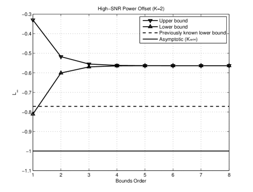
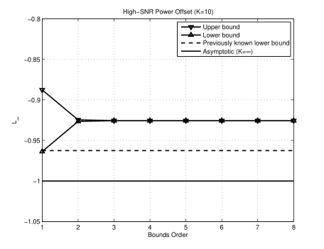
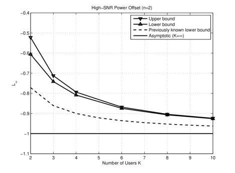
In Figures 2 and 3 we present the high-SNR power offset bounds of Proposition 3 in the special case of Rayleigh fading (real and imaginary parts are independent Gaussian random variables with zero mean and variance $1/\sqrt{2}$), for $K=2$ and $K=10$ users per-cell respectively. The curves are produced by Monte Carlo simulation with $10^{5}$ samples. The figures include also the lower bound of [11], see (38), and the asymptotic results (and lower bound) for large number of users per-cell $\mathcal{L}_{\infty}=-1$ (achieved by taking $K$ to infinity in (38)). Examining the figures it is observed that the new bounds are getting tighter with their order $n$ and that the new lower bound is tighter than (38) already for $n=2$. Moreover, fixing the order $n$, the new bounds are getting tighter with the number of users per-cell $K$. This observation is also evident from Fig. 4, where the bounds are plotted for a fixed order $n=2$ versus the number of users per-cell $K$. Finally, since the upper bound of Fig. 2 is negative, we conclude that the presence of Rayleigh fading is beneficial over non-fading channels in the high-SNR region already for $K=2$. (See [11] for a similar conclusion in the low-SNR region.)

III Background, Previous Results and Bounds

In this section we briefly summarize previous work on the “soft-handoff” uplink cellular model introduced in [10][11]. For conciseness, we restrict the discussion to the case where $\pi_{a}=\pi_{b}$. Most of the results in the sequel can be extended to include the general case where $\pi_{a}\neq\pi_{b}$.

Starting with non-fading channels (i.e., when $\pi_{a}$ and $\pi_{b}$ are singletons at 1), the per-cell sum-rate capacity of the uplink channel is given for $M\rightarrow\infty$ by [11]

$$R_{\mathrm{nf}}=\log\left(\frac{1+2P+\sqrt{1+4P}}{2}\right)\ .$$ (20)

This rate is achieved by any symmetric intra-cell protocol with average transmit power of $P$ (e.g. intra-cell TDMA, and WB protocols). It is noted that the same result holds also for phase fading processes [13].

The extreme SNR characterization of (20) is summarized for the non-fading setup by

$$S_{0}=\frac{4}{3}\,,\quad\frac{E_{b}}{N_{0}}_{\min}=\frac{\log 2}{2}\,,\quad S_{\infty}=1\,,\quad\mathcal{L}_{\infty}=0\,.$$ (21)

Returning to the flat fading setup, the channel coefficients are taken as i.i.d.  random variables, denoting by

$$\begin{aligned} m_{1}&\triangleq{\mathbb{E}}(a_{m,k})={\mathbb{E}}(b_{m,k})\quad;\quad m_{2}\triangleq{\mathbb{E}}(\left|a_{m,k}\right|^{2})={\mathbb{E}}(\left|b_{m,k}\right|^{2})\,\quad\\ m_{4}&\triangleq{\mathbb{E}}(\left|a_{m,k}\right|^{4})={\mathbb{E}}(\left|b_{m,k}\right|^{4})\quad;\quad\mathcal{K}\triangleq\frac{m_{4}}{m_{2}^{2}}\end{aligned}\quad,\ \forall\ m,k$$ (22)

the mean, second power moment, fourth power moment and the kurtosis of an individual fading coefficient.

The per-cell sum-rate capacity of the WB scheme with fixed $P$ and increasing number of users and cells $M,K\rightarrow\infty$, is given by [11]333Here, the number of users $K$ is taken to infinity and then the number of cells $M$ is taken to infinity.

$$R_{\mathrm{wb-f}}=\log\left(\frac{1+2Pm_{2}+\sqrt{1+4Pm_{2}+4P^{2}(m_{2}^{2}-\left|m_{1}\right|^{4}})}{2}\right)\ .$$ (23)

The rate is maximized for a zero mean fading distribution and is given by

$$R_{\mathrm{wb-f}}=\log(1+2m_{2}P)\ .$$ (24)

Comparing (20) and (24) (with $m_{2}=1$), it follows that the presence of fading is beneficial in case the number of users is large. We note that (23) is also shown in [11] to upper bound the respective rate for any finite number of users $K$.

Returning to the intra-cell TDMA ($K=1$), for which standard random matrix theory is not suitable (see Sec. II-B), the powerful moment bounding technique employed in [27] for the Wyner model, can be utilized to obtain lower and upper bounds on the per-cell sum-rate.

An alternative approach which replaces the role of the singular values with the diagonal elements of the Cholesky decomposition of the the matrix $\boldsymbol{G}_{M}$, was presented by Narula [14] for a two diagonal nonzero channel matrix $\boldsymbol{H}_{M}$ whose entries are i.i.d. zero-mean complex Gaussian (Rayleigh fading). Originally, Narula had studied the capacity of a time varying two taps inter-symbol-interference (ISI) channel, where the channel coefficients are i.i.d. zero-mean complex Gaussian. With the above assumptions regarding the ISI channel coefficients it is easy to verify that the capacity of this model is equal to the per-cell sum-rate capacity of an uplink intra-cell TDMA scheme employed in the “soft-handoff” model.

Following [14], we use the Cholesky decomposition applied to the covariance matrix of the uplink intra-cell TDMA scheme output vector $\boldsymbol{G}_{M}=\boldsymbol{L}_{M}\boldsymbol{D}_{M}\boldsymbol{U}_{M}$, where $\boldsymbol{L}_{M}$ (resp. $\boldsymbol{U}_{M}$) is a lower triangular (resp. upper triangular) matrix with 1 on the diagonal. The diagonal entries of $\boldsymbol{G}_{M}$ are given (with $K=1$) by

$$d_{m}=1+P\left|a_{m}\right|^{2}+P\left|b_{m}\right|^{2}\left(1-P\frac{\left|a_{m-1}\right|^{2}}{d_{m-1}}\right)\ ,\ m=2,\ldots,M\ ,$$ (25)

where the initial condition of (25) is $d_{1}=1+P\left|a_{1}\right|^{2}+P\left|b_{1}\right|^{2}$. Thus, the diagonal entries $\{d_{m}\}$ form a discrete-time continuous space Markov chain; Narula’s main observation was that this chain possesses a unique ergodic stationary distribution, given by

$$f_{d}(x)=\frac{\log(x)e^{-\frac{x}{P}}}{\text{Ei}\left(\frac{1}{\bar{P}}\right)P}\quad;\quad x\geq 1\ ,$$ (26)

where $\text{Ei}(x)=\int_{x}^{\infty}\frac{\exp(-t)}{t}dt$ is the exponential integral function. Further, as is proved in [14], the strong law of large numbers (SLLN) holds for the sequence $\{\log{d_{m}}\}$ as $M\rightarrow\infty$. Hence, the average per-cell sum-rate capacity of the intra-cell TDMA scheme ($K=1$) can be expressed as

$\displaystyle R_{\mathrm{tdma-f}}$ $\displaystyle=\lim_{M\rightarrow\infty}{\mathbb{E}}\left(\frac{1}{M}\log\det\boldsymbol{G}_{M}\right)$ (27)
$\displaystyle=\lim_{M\rightarrow\infty}{\mathbb{E}}\left(\frac{1}{M}\log\det\left(\boldsymbol{L}_{M}\boldsymbol{D}_{M}\boldsymbol{U}_{M}\right)\right)$
$\displaystyle=\lim_{M\rightarrow\infty}{\mathbb{E}}\left(\frac{1}{M}\sum_{m=0}^{M}\log d_{m}\right)={\mathbb{E}}_{\pi_{d}}\left(\log d\right)\ ,$

where the last expectation is taken with respect to $f_{d}(x)$, as defined in (26). In particular,

$$R_{\mathrm{tdma-f}}=\int_{1}^{\infty}\frac{(\log(x))^{2}e^{-\frac{x}{P}}}{\text{Ei}\left(\frac{1}{P}\right)P}dx\ .$$ (28)

Narula’s approach is based on an explicit calculation of the invariant distribution $f_{d}$, and is thus tied to Rayleigh fading. Modifications of key parameters (such as the entries’ PDF, and the number of nonzero diagonals) lead to analytically intractable expressions.

Another result derived by following the footsteps of [14] is an upper bound on the per-cell sum-rate of the WB scheme with finite $K$ and infinite number of cells $M\rightarrow\infty$, in the presence of a general fading distribution, given by

$$R_{\mathrm{wbk-f}}\leq\log\left(\frac{1+2Pm_{2}+\sqrt{1+4Pm_{2}+4P^{2}\left(1-\frac{1}{K}\right)\left(m_{2}^{2}-\left|m_{1}\right|^{4}\right)}}{2}\right)\ .$$ (29)

and in the special case of zero mean unit power ($m_{1}=0,\ m_{2}=1$) fading distribution (e.g. Rayleigh fading) the bound reduces to

$$R_{\mathrm{wbk-f}}\leq\log\left(\frac{1+2P+\sqrt{(1+2P)^{2}-(4P^{2}/K)}}{2}\right)\ .$$ (30)

This result which is proved in [14] for $K=1$ (intra-cell TDMA protocol) and expanded to an arbitrary $K$ in [15], is derived by noting that the average of the determinant of the received vector covariance matrix $\boldsymbol{G}_{M}$ can be recursively expressed by

$${\mathbb{E}}(\det\boldsymbol{G}_{m})=A\ {\mathbb{E}}(\det\boldsymbol{G}_{m-1})-B\ {\mathbb{E}}(\det\boldsymbol{G}_{m-2})\ ;\ m=3,\ldots,M\ ,$$ (31)

with initial conditions

$${\mathbb{E}}(\det\boldsymbol{G}_{1})=A\quad;\quad{\mathbb{E}}(\det\boldsymbol{G}_{2})=A^{2}-B\ ,$$ (32)

where

$$A=1+2Pm_{2}\quad;\quad B=\frac{P^{2}}{K}\left(m_{2}^{2}+(K-1)\left|m_{1}\right|^{4}\right)\ .$$ (33)

See Appendix -E for more details. The solution to (31) is given by

$${\mathbb{E}}(\det\boldsymbol{G}_{m})=\varphi\ r^{m}-\phi\ s^{m}\ ,$$ (34)

where

$$r=\frac{1}{2}\left(A+\sqrt{A^{2}-4B}\right)\quad;\quad s=\frac{1}{2}\left(A-\sqrt{A^{2}-4B}\right)\ ,$$ (35)

are real and positive, and $\varphi$, $\phi$ are determined by the initial conditions (32). Finally, (29) is derived by the following set of inequalities

$$R_{\mathrm{wbk-f}}=\lim_{M\rightarrow\infty}\frac{1}{M}{\mathbb{E}}\left(\log\det\boldsymbol{G}_{M}\right)\leq\lim_{M\rightarrow\infty}\frac{1}{M}\log{\mathbb{E}}\left(\det\boldsymbol{G}_{M}\right)\ =\log r\ ,$$ (36)

where the inequality is due to Jensen’s inequality, and the last equality follows from the fact that $r>s$, and $M\rightarrow\infty$. In the case of $K=1$, the upper bound of (30) coincides with the per-cell sum-rate capacity of the non-fading setup (20). Thus, the presence of Rayleigh fading decreases the rates of the intra-cell TDMA protocol supported by the “soft-handoff” model. Nevertheless, it is shown in [11] that already for $K=2$ the presence of fading may be beneficial at least for low SNR values. The tightness of the bound is demonstrated by noting the for $K\rightarrow\infty$ it coincides with the asymptotic expression of (23).

The extreme SNR characterization of the WB rate for $M\rightarrow\infty$ in the presence of a general fading distribution is summarized by [11]

$$\begin{array}[]{cc}S_{0}=\frac{2}{\frac{\mathcal{K}}{2K}+\frac{\left|m_{1}\right|^{4}}{2m_{2}^{2}}+1}\ ;&\frac{E_{b}}{N_{0}}_{\min}=\frac{\log 2}{2m_{2}}\\ S_{\infty}\leq 1\ ;&-\log_{2}\left(m_{2}+\sqrt{\left(1-\frac{1}{K}\right)\left(m_{2}^{2}-\left|m_{1}\right|^{4}\right)}\right)\leq\mathcal{L}_{\infty}\ .\end{array}$$ (37)

The bounds of the high-SNR parameters are tight for $K\gg 1$. For the special case of Rayleigh fading the extreme SNR characterization are given by [11]

$$\begin{array}[]{cc}S_{0}=\frac{2}{1+\frac{1}{K}}\ ;&\frac{E_{b}}{N_{0}}_{\min}=\frac{\log 2}{2}\\ S_{\infty}=1\ ;&-\log_{2}\left(1+\sqrt{1-\frac{1}{K}}\right)\leq\mathcal{L}_{\infty}\leq\frac{\gamma}{\log 2}\ ,\end{array}$$ (38)

where $\gamma\approx 0.5772$ is the Euler-Mascheroni constant. It is noted that the right inequality of the high-SNR power offset is tight for $K=1$, while the left inequality is tight for $K\gg 1$. The beneficial effects of Rayleigh fading and increasing number of users are evident when compared to the non-fading extreme-SNR parameters of the respective non-fading setup (21).

To conclude this section we emphasize that calculating exact expressions for the high-SNR parameters of the WB protocol rate with finite number of users per-cell and general fading distribution remains an open problem.

IV Applications

In this section we present several applications of the main results presented in this work (see Section II-D).

Intra-Cell TDMA and Rayleigh Fading

Assuming that only one user is active per-cell $K=1$ and symmetric Rayleigh fading channels (i.e. $\pi_{\left|a\right|^{2}}$ and $\pi_{\left|b\right|^{2}}$ are exponential distributions with parameter 1), the high-SNR power offset is given according to Theorem 1, by

$$\mathcal{L}_{\infty}=-\max\left({\mathbb{E}}(\log_{2}\left|a\right|^{2}),{\mathbb{E}}(\log_{2}\left|b\right|^{2})\right)=\frac{-1}{\log 2}\int_{0}^{\infty}e^{-x}\log x\ dx=\frac{\gamma}{\log 2}$$ (39)

where the last equality is due to [28, pp. 567, formula 4.331.1]. Obviously this result coincides with the high-SNR power-offset derived by applying the definition of $\mathcal{L}_{\infty}$ (see (13)) directly to the exact expression derived in [14] (see expression (28)).

Note that the same result holds if an attenuation factor is added to one of the fading paths, e.g. $\tilde{b}_{m}=\alpha b_{m}$ where $b_{m}\sim\mathcal{CN}(0,1)$ and $\alpha\in[0,1]$; this follows directly from Theorem 1, but not from [14], which requires symmetric fading paths (i.e. $\alpha=1$).

Intra-Cell TDMA and General Fading Statistic

Consider the following single user single-input single-output (SISO) flat fading channel for an arbitrary time index

$$y=ax+n\ ,$$ (40)

where $x$ is the input signal $x\sim\mathcal{CN}(0,P)$, and $n$ is the additive circularly symmetric Gaussian noise $n\sim\mathcal{CN}(0,1)$. In addition, $a$ is the fading coefficient $a\sim\pi_{a}$ satisfying conditions (H1)…(H3) and known only to the receiver (receiver CSI). Assuming that the fading process is also ergodic in the time domain, the ergodic capacity of the channel is given by [24]

$$C={\mathbb{E}}_{\pi_{a}}\log(1+P\left|a\right|^{2})\ ,$$ (41)

where the expectation is taken over the fading distribution $\pi_{a}$. Accordingly, under the mild conditions (H1)…(H3), the high-SNR regime of this channel is characterized by

$$\mathcal{S}_{\infty}=1\quad;\quad\mathcal{L}_{\infty}=-{\mathbb{E}}_{\pi_{a}}\log_{2}\left|a\right|^{2}\ .$$ (42)

Using Theorem 1, we can now establish the following analogy between the multi-cell setup and the SISO channel at hand.

Corollary 4

The high-SNR characterization of the intra-cell TDMA per-cell sum-rate supported by the “soft-handoff” setup with fading distributions $\pi_{a},\pi_{b}$ such that ${\mathbb{E}}_{\pi_{a}}\log_{2}\left|a\right|^{2}>{\mathbb{E}}_{\pi_{b}}\log_{2}\left|b\right|^{2}$, coincides with those of a scalar single-user fading channel with fading distribution $\pi_{a}$.

This observation allows us to use the vast body of work done for the celebrated scalar flat fading channel [24]. In particular, the high-SNR characterization of flat fading channels with the following fading statistics have been considered in previous works: (a) Rayleigh distribution, (b) Rice distribution, (c) log-normal distribution, and (d) Nakagami distribution (see [24] and references therein).

Intra-Cell TDMA and Opportunistic Scheduling

Throughout this work we have assumed that the instantaneous channel state information is known to the MCP receiver only. Here we further assume that some sort of ideal feedback channel is available between the MCP receiver and the $K$ mobile users included in each cell. This feedback channel is used to schedule the “best” local user in each cell for transmission during the current time slot444See [29] for a similar scheduling deployed in the Wyner cellular uplink channel.. In other words, in each cell the user with the strongest channel fade towards the BS located on the right boundary of each cell is scheduled for transmission555Since the right most cell indexed (M+1), has no BS on its right boundary it randomly schedules a user for transmission. with power $P$. Hence, the index of the selected user in the $m$th cell reads

$$\tilde{k}_{m}=\underset{k=1,2,\ldots K}{\mathrm{argmax}}\left|a_{m,k}\right|^{2}\quad m=1,2,\ldots,M\ .$$ (43)

The resulting $M\times(M+1)$ channel transfer matrix $\boldsymbol{\tilde{H}}_{M}$ of this scheduling scheme is a two diagonal matrix with independent entries. The probability density function of the main diagonal i.i.d. entries’ amplitudes is given by

$$d\pi_{K,\left|a\right|^{2}}=K\pi_{\left|a\right|^{2}}^{K-1}d\pi_{\left|a\right|^{2}}\ ,$$ (44)

following the maximum order statistics [30]. On the other hand, the i.i.d. entries of the second non-zero diagonal are distributed according to the original fading statistics $\pi_{b}$.

Assuming that $\pi_{K,\left|a\right|^{2}}$ and $\pi_{b}$ satisfy conditions (H1)…(H3), we can apply Theorem 1 in order to derive the high-SNR characteristics of the per-cell sum-rate achievable by this opportunistic scheduling

$$\mathcal{S}_{\infty}=1\quad;\quad\mathcal{L}_{\infty}=-\max\left({\mathbb{E}}_{\pi_{K,\left|a\right|^{2}}}(\log_{2}y),{\mathbb{E}}_{\pi_{b}}(\log_{2}\left|b\right|^{2})\right)\ .$$ (45)

For Rayleigh fading channels and in the case where the number of users per-cell is large $K\gg 1$, we can use the well known fact that the square of the maximum of the $K$ amplitudes behaves like $\log K$ with high-probability (see [31]). Hence, the rate high-SNR power offset of this scheme is

$$\mathcal{L}_{\infty}\approx-\log_{2}\log K\ ,$$ (46)

revealing a multi-user diversity gain of $\log\log K$. It is noted that allowing additional power control to this scheme will yield better performances. However, we are unable to apply Theorem 1 for this situation. Finally, choosing the BS located on the right boundary of the cell is arbitrary; taken the BS located on the left boundary of the cell yields the same results.

V Concluding Remarks

In this paper we study the high-SNR characterization of the per-cell sum-rate capacity of the “soft-handoff” uplink cellular channel with multi-cell processing. Taking advantage of the special topology induced by the setup, the problem reduces to the study of the spectrum of certain large random Hermitian Jacobi matrices. For the intra-cell TDMA protocol where only one user is active simultaneously per-cell we provide an exact closed form expression for the per-cell sum-rate high-SNR power offset for rather general fading distribution. Examining the result, it is concluded that in the high-SNR regime, the rate of the cellular setup at hand is equivalent to the one of a single user SISO channel with similar fading statistics.

Turning to the capacity achieving WB protocol, where all $K$ users are active simultaneously in each cell, we derive a series of lower and upper bounds to the rate. These bounds are shown (via Monte-Carlo simulations) to be tighter than previously known bounds.

Note that in Theorem 2 points a) and c) and in Proposition 3, we take the fading coefficients relative to the users of one cell to be independent. Those results continue to be true if we assume correlation between the fading coefficients relative to the users of the same cell (but independence between cells). The proof is identical to the proof given in the paper.

Some of the analysis reported here can be extended to include the case where $\boldsymbol{G}_{M}$ is $(2p-1)$-diagonal for some $p>2$ (e.g. $p=3$ for the channel matrix of the Wyner model), using an adaptation of the “Thouless formula for the strip” derived originally in [32]. Using this approach, bounds similar to those of Prop. 3 may be provided on the rate. Details will appear elsewhere [33].

Acknowledgments

N. L. was partially supported by the fund for promotion of research at the Technion.

O. S. was partially supported by a Marie Curie Outgoing International Fellowship within the 6th European Community Framework Program.

S. S. was partially supported by the REMON Consortium and NEWCOM++.

O. Z. was partially supported by NSF grant number DMS-0503775; Part of this work was done while he was with the Department of Electrical Engineering, Technion.

We thank David Bitton for his help with the implementation of the Monte Carlo simulation used in Section II-D (application of Proposition 3).

-A Proof of Theorem 1

In order to streamline the proof we somewhat modify notation. We consider two random sequences of complex numbers $(a_{n})$ and $(b_{n})$. The $(a_{n})$ (resp. $(b_{n})$) are i.i.d of law $\pi_{a}$ (resp. $\pi_{b}$) and the $(a_{n})$ are independent of the $(b_{n})$. We set $\Omega\triangleq((a_{n}),(b_{n}))$. We denote by ${\mathbb{P}}$ the probability associated with those random sequences and by ${\mathbb{E}}$ the associated expectation. For a given integer $n$, we consider a channel transfer matrix $\boldsymbol{H}_{M}$ of size $M\times(M+1)$.

$$\boldsymbol{H}_{M}=\begin{pmatrix}a_{1}&b_{1}&0&\cdots&0\\ 0&\ddots&\ddots&\ddots&\vdots\\ \vdots&\ddots&\ddots&\ddots&0\\ 0&\cdots&0&a_{M}&b_{M}\\ \end{pmatrix}.$$

We consider the following variable

$$\mathcal{C}_{M}(P)=\frac{1}{M}\operatorname{tr}\left\{\log\left(I+P\boldsymbol{H}_{M}\boldsymbol{H}_{M}^{\dagger}\right)\right\}.$$

Note that,

$$\boldsymbol{H}_{M}\boldsymbol{H}_{M}^{\dagger}=\begin{pmatrix}\left|a_{1}\right|^{2}+\left|b_{1}\right|^{2}&a_{2}^{\dagger}b_{1}&0&\cdots&0\\ a_{2}b_{1}^{\dagger}&\left|a_{2}\right|^{2}+\left|b_{2}\right|^{2}&a_{3}^{\dagger}b_{2}&\ddots&\vdots\\ 0&\ddots&\ddots&\ddots&0\\ \vdots&\ddots&\ddots&\ddots&a_{M}^{\dagger}b_{M-1}\\ 0&\cdots&0&a_{M}b_{M-1}^{\dagger}&\left|a_{M}\right|^{2}+\left|b_{M}\right|^{2}\\ \end{pmatrix}.$$

With this notation, as explained in Section II-D, Theorem 1 follows from the following.

Theorem 5

[$K=1$] Assume (H1) and (H2) .

  1. a)

    For every $\rho>0$, $\mathcal{C}_{M}(P)$ converges ${\mathbb{P}}$-a.s as $M$ goes to infinity. We call the limit $\mathcal{C}(P)$.

  2. b)

    Further assume [(H3) or (H3’)]. As $\rho$ goes to infinity,

    $$\mathcal{C}(P)=\log P+2\max\left({\mathbb{E}}_{\pi_{a}}\log\left|x\right|;{\mathbb{E}}_{\pi_{b}}\log\left|x\right|\right)+o(1).$$

Proof of Theorem 5 Without loss of generality, in the proof we can assume

  1. (H5)

    ${\mathbb{E}}_{\pi_{a}}\log\left|x\right|\leq{\mathbb{E}}_{\pi_{b}}\log\left|x\right|$.

Indeed, we may exchange the role of entries $a_{i}$ and $b_{i}$ for $1\leq i\leq M$ by a right-left reflection, namely the transformation $\hat{a}_{j}=b_{M-j+1}$, $\hat{b}_{j}=a_{M-j+1}$, $1\leq j\leq M$.

For part a), only (H1) and (H2) are needed. Since part a) is a consequence of general facts concerning products of random matrices and does not use much of the special structure in the problem, we bring it in Appendix -D.

Part b) uses the theory of Markov chains and is specific to the particular matrix $\boldsymbol{H}_{M}$. We note that as a by product of this approach, we obtain a second proof of part a), however under the additional assumption [(H3) or (H3’)]. We provide a proof of Theorem 5 under the assumptions (H1), (H2) and [(H3) or (H3’)] in Appendices -A and -B.

The structure of the proof is as follows. We first introduce an auxiliary sequence which allows us to reformulate the problem in terms of a special Markov chain. The study of the latter, which forms the bulk of the proof of Theorem 5, is carried out in Section -B.

-A1 Auxiliary sequence

We begin with a technical lemma.

Lemma 6

Assume (H2). ${\mathbb{P}}$-a.s, $\boldsymbol{H}_{M}\boldsymbol{H}_{M}^{\dagger}$ does not have multiple eigenvalues.

Proof.

We let $D$ denote the discriminant of $\boldsymbol{H}_{M}\boldsymbol{H}_{M}^{\dagger}$, it is a polynomial in
$\{\left|a_{i}\right|^{2}+\left|b_{i}\right|^{2},a_{i+1}b_{i}^{\dagger},a_{i+1}^{\dagger}b_{i}\}$ which vanishes when there is a multiple eigenvalue. Therefore, it is a polynomial in $\Re a_{i}$, $\Im a_{i}$, $\Re b_{i}$ and $\Im b_{i}$ It is not identically 0 because for $b_{i}=0$ and $a_{i}=i$, the eigenvalues of $\boldsymbol{H}_{M}\boldsymbol{H}_{M}^{\dagger}$ are distinct. The result follows directly from the following lemma which is an easy consequence of Fubini’s theorem. ∎

Lemma 7

Let $Q$ be a function from ${\mathbb{C}}^{n}$ to ${\mathbb{C}}$. We assume that $Q$ is not identically 0 and that $Q(z_{1},\ldots,z_{n})$ is a polynomial in the $\Re z_{i}$ and the $\Im z_{i}$. Then the set of the roots of $Q$ has Lebesgue measure 0.

In the sequel, we denote by $\lambda_{1}\geq\ldots\geq\lambda_{M}$ the ordered eigenvalues of $\boldsymbol{H}_{M}\boldsymbol{H}_{M}^{\dagger}$. For a given $\lambda$, we consider the following sequence (indexed by $n$) of complex numbers (the dependence in $\lambda$ will only be mentioned when it is relevant): $x_{0}=0$, $x_{1}=1$, and for $n\geq 1$,

$$a_{n}b_{n-1}^{\dagger}x_{n-1}+(\left|a_{n}\right|^{2}+\left|b_{n}\right|^{2})x_{n}+a_{n+1}^{\dagger}b_{n}x_{n+1}=\lambda x_{n},$$

that is

$\displaystyle x_{n+1}=\frac{\lambda-\left|a_{n}\right|^{2}-\left|b_{n}\right|^{2}}{a_{n+1}^{\dagger}b_{n}}x_{n}-\frac{a_{n}b_{n-1}^{\dagger}}{a_{n+1}^{\dagger}b_{n}}x_{n-1}.$ (47)

Note that $x_{M+1}(\lambda)=0$ if and only if $\lambda$ is an eigenvalue of $\boldsymbol{H}_{M}\boldsymbol{H}_{M}^{\dagger}$. Moreover, $x_{n+1}$ is a polynomial in $\lambda$ of degree $n$ with highest coefficient $1/\prod_{i=1}^{n}(a_{i+1}^{\dagger}{b_{i}})$. One can thus write using Lemma 6

$$x_{n+1}(\lambda)=\prod_{i=1}^{n}(a_{i+1}^{\dagger}{b_{i}})^{-1}\prod_{i=1}^{n}(\lambda-\lambda_{i})\ \ \ \ {\mathbb{P}}-\textrm{a.s},$$

Hence, for $\lambda=-1/P$,

$\displaystyle\mathcal{C}_{M}(P)=\log(P)+\frac{1}{M}\log\left|x_{M+1}(\lambda)\right|+\frac{1}{M}\sum_{i=1}^{M}\log\left|a_{i+1}b_{i}\right|\ \ \ \ \ \ \ {\mathbb{P}}-\textrm{a.s}.$ (48)

By the Law of Large Numbers (LLN),

$$\lim_{M\rightarrow\infty}\frac{1}{M}\sum_{i=1}^{M}\log\left|a_{i+1}b_{i}\right|={\mathbb{E}}_{\pi_{a}}\log\left|x\right|+{\mathbb{E}}_{\pi_{b}}\log\left|x\right|\ \ \ \ {\mathbb{P}}-\textrm{a.s}.$$

Because of (48), to prove Theorem 5, we only need to show the following lemma.

Lemma 8

Assume (H1), (H2) and [(H3) or (H3’)]

  1. a)

    For every $\lambda<0$, $\frac{1}{n}\log\left|x_{n+1}(\lambda)\right|$ converges ${\mathbb{P}}$-a.s as $n$ goes to infinity. The limit is $\gamma(\lambda)$, the Lyapunov exponent defined by (62).

  2. b)

    Assume further (H5). Then $\gamma(\lambda)$ converges to ${\mathbb{E}}_{\pi_{b}}\log\left|x\right|-{\mathbb{E}}_{\pi_{a}}\log\left|x\right|$ as $\lambda$ goes to 0.

-A2 Reduction to a Markov chain

To prove Lemma 8, we take $c_{n}\triangleq x_{n}/x_{n-1}$, for $n\geq 2$. Note that by (47) and (H2), ${\mathbb{P}}$-a.s, $x_{n}\neq 0$, hence $c_{n}$ is well defined and non-zero. By (47), we get

$$c_{n+1}=\frac{\lambda-\left|a_{n}\right|^{2}-\left|b_{n}\right|^{2}}{a_{n+1}^{\dagger}b_{n}}-\frac{a_{n}b_{n-1}^{\dagger}}{c_{n}a_{n+1}^{\dagger}b_{n}}.$$

Let $d_{n}=c_{n}a_{n}^{\dagger}b_{n-1}$. Then,

$$d_{n+1}=\lambda-\left|a_{n}\right|^{2}-\left|b_{n}\right|^{2}-\frac{\left|a_{n}\right|^{2}\left|b_{n-1}\right|^{2}}{d_{n}}=\lambda-\left|b_{n}\right|^{2}-\left|a_{n}\right|^{2}\left(1+\frac{\left|b_{n-1}\right|^{2}}{d_{n}}\right).$$

Let $e_{n}=\left(1+\frac{\left|b_{n-1}\right|^{2}}{d_{n}}\right)$. Then $d_{n+1}=\lambda-\left|b_{n}\right|^{2}-\left|a_{n}\right|^{2}e_{n}$, and

$\displaystyle e_{n}=\frac{-\lambda+\left|a_{n-1}\right|^{2}e_{n-1}}{-\lambda+\left|b_{n-1}\right|^{2}+\left|a_{n-1}\right|^{2}e_{n-1}},$ (49)

with the initial conditions,

$$c_{2}=\frac{\lambda-\left|a_{1}\right|^{2}-\left|b_{1}\right|^{2}}{a_{2}^{\dagger}b_{1}};$$
$$d_{2}=\lambda-\left|b_{1}\right|^{2}-\left|a_{1}\right|^{2}.$$

$d_{2}\in{\mathbb{R}}$ and $d_{2}<-\left|b_{1}\right|^{2}$, hence, $0<e_{2}<1$. From (49) we conclude that for all $n$, $e_{n}\in{\mathbb{R}}$ and $0<e_{n}<1$. Now, for all $n$,

$$c_{n}=\frac{d_{n}}{a_{n}^{\dagger}b_{n-1}}=\frac{b_{n-1}^{\dagger}}{a_{n}}^{\dagger}\frac{1}{e_{n}-1}.$$

Then,

$$\begin{split}\frac{1}{n}\log\left|x_{n+1}\right|&=\frac{1}{n}\sum_{i=2}^{n+1}\log\left|c_{i}\right|\\ &=\frac{1}{n}\sum_{i=2}^{n+1}\left(\log\left|\frac{b_{i-1}}{{a_{i}}}\right|-\log(1-e_{i})\right)\\ \end{split}$$ (50)

$\frac{1}{n}\sum_{i=2}^{n+1}\log\left|\frac{b_{i-1}}{{a_{i}}}\right|$ converges to ${\mathbb{E}}_{\pi_{b}}\log\left|x\right|-{\mathbb{E}}_{\pi_{a}}\log\left|x\right|$ by the LLN. We now study in details the Markov chain $e_{n}$.

-B Study of the Markov chain $e_{n}$ and proof of Lemma 8

For simplicity, we write $\delta\triangleq-\lambda$ and we re-index the chain so that it starts from $e_{0}$. As in (49),

$\displaystyle e_{n}=\frac{\delta+\left|a_{n-1}\right|^{2}e_{n-1}}{\delta+\left|b_{n-1}\right|^{2}+\left|a_{n-1}\right|^{2}e_{n-1}}.$ (51)

We denote by ${\mathbb{P}}_{e_{0}}$ the law of the sequence starting from $e_{0}$ and by ${\mathbb{E}}_{e_{0}}$ the associated expectation.

Proposition 9

Assume (H2) and [(H3) or (H3’)]. The Markov chain $e_{n}$ has a unique stationary probability, say, $\mu_{\delta}$ and for $s\in{\mathbb{L}}^{1}(\mu_{\delta})$, for every starting point $e_{0}\in[0,1]$, ${\mathbb{P}}_{e_{0}}$-a.s,

$$\frac{1}{n}\sum_{i=0}^{n}s(e_{i})\xrightarrow[n\rightarrow\infty]{}\int sd\mu_{\delta}.$$
Proof.

We start with two lemmas that will be proved later on.

Lemma 10

For $\alpha,\beta,\delta\in{\mathbb{R}}^{+}$, we define the function $\phi_{\alpha,\beta}$ (we suppress $\delta$ from the notation) such that for $e\in[0,1]$

$$\phi_{\alpha,\beta}(e)=\frac{\delta+\alpha e}{\delta+\beta+\alpha e}.$$

For any given $e\in[0,1]$, we define the sequence $(\theta_{n}(e))$ by $\theta_{0}=e$ and for $n\geq 1$, $\theta_{n}(e)=\phi_{\alpha,\beta}(\theta_{n-1}(e))$. Then, $\phi_{\alpha,\beta}$ has exactly one fixed point in $[0,1]$, say $\kappa_{\alpha,\beta}$, and $\theta_{n}(e)$ converges to $\kappa_{\alpha,\beta}$. Moreover, the convergence is uniform in the starting point in the following sense:

$$(\forall\varepsilon>0)(\exists n_{0}\in{\mathbb{N}})(\forall e\in[0,1])(\forall n\geq n_{0})(\left|\theta_{n}(e)-\kappa_{\alpha,\beta}\right|<\varepsilon).$$

Finally if $\alpha_{1}<\alpha_{2}$ and $\beta_{1}>\beta_{2}$, then $\kappa_{\alpha_{1},\beta_{1}}<\kappa_{\alpha_{2},\beta_{2}}$.

Lemma 11

Assume (H2) and [(H3) or (H3’)].

  1. a)

    For $e_{0}\in[0,1]$, there exist two sequences $(\theta_{n}^{1}(e_{0}))$ and $(\theta_{n}^{2}(e_{0}))$ in $[0,1]$ such that the law of $e_{n}$ under ${\mathbb{P}}_{e_{0}}$ and the Lebesgue-measure on $[(\theta_{n}^{1}(e_{0})),(\theta_{n}^{2}(e_{0}))]$ are mutually absolutely continuous.

  2. b)

    $(\theta_{n}^{1}(e_{0}))$ and $(\theta_{n}^{2}(e_{0}))$ converge to, say $\Theta^{1}$ and $\Theta^{2}$ respectively, $\Theta^{1}$ and $\Theta^{2}$ are independent of $e_{0}$ and $\Theta^{1}<\Theta^{2}$. Finally, the convergence is uniform in the starting point in the sense of Lemma 10.

  3. c)

    If $e_{0}\in[\Theta^{1},\Theta^{2}]$, then for all $n$, the law of $e_{n}$ under ${\mathbb{P}}_{e_{0}}$ is absolutely continuous with respect to the Lebesgue-measure on $[\Theta^{1},\Theta^{2}]$.

We recall some definitions from the theory of Harris Markov chains, which will be used extensively in the proof. We refer the reader to [34] for the relevant background.

Definition 12

Denote by $(r_{n})$ a Markov chain on $I$ an interval of ${\mathbb{R}}$. Set $l$ a probability measure on $I$, it is an irreducibility measure if for all measurable set $A$ such that $l(A)>0$ and for all $r_{0}\in I$

$$(\exists n)\ {\mathbb{P}}_{r_{0}}(r_{n}\in A)>0.$$

$l$ is a maximal irreducibility measure if it satisfies the following conditions:

  • $l$ is an irreducibility measure.

  • For any other irreducibility measure $l^{\prime}$, $l^{\prime}$ is absolutely continuous with respect to $l$.

  • If $l(A)=0$ then $l\{r_{0}:(\exists n)\ {\mathbb{P}}_{r_{0}}(r_{n}\in A)>0\}=0$.

  • For any irreducibility measure $l^{\prime}$, $l$ is equivalent to

    $$\int_{I}l^{\prime}(dr_{0})\sum_{i=0}^{\infty}\frac{1}{2^{i}}{\mathbb{P}}_{r_{0}}(r_{i}\in\cdot).$$
Definition 13

Denote by $(r_{n})$ a Markov chain on $I$ an interval of ${\mathbb{R}}$. A set $A$ is called Harris recurrent if for all $r_{0}\in A$, ${\mathbb{P}}_{r_{0}}$-a.s, the chain $r_{n}$ visits $A$ an infinite number of times. The chain $(r_{n})$ is called Harris recurrent if given a maximal irreducibility measure $l$, every measurable set $A$ such that $l(A)>0$ is Harris recurrent.

Definition 14

Denote by $(r_{n})$ a Markov chain on $I$ an interval of ${\mathbb{R}}$. Denote by $l$ a maximal irreducibility measure. For every measurable set $A$ such that $l(A)>0$ we denote by $\tau_{A}$ the time when the chain $(r_{n})$ enters $A$. A measurable set $B$ is called regular if for every measurable set $A$ such that $l(A)>0$,

$$\sup_{r_{0}\in B}{\mathbb{E}}_{r_{0}}(\tau_{A})<\infty.$$
Definition 15

Denote by $(r_{n})$ a Markov chain on $I$ an interval of ${\mathbb{R}}$. Denote by $A$ and $B$ two measurable sets. We say that $B$ is uniformly accessible from $A$ if there exists an $\varepsilon>0$ such that

$$\inf_{r_{0}\in A}{\mathbb{P}}_{r_{0}}((\exists n)\ r_{n}\in B)\geq\varepsilon.$$

We continue with the proof of Proposition 9. Denote by $l$ the Lebesgue-measure on $[\Theta^{1},\Theta^{2}]$. By [34, Theorem 17.0.1], it is enough to prove that the Markov chain $e_{n}$ is $l$-irreducible, positive Harris with invariant probability $\mu_{\delta}$. Denote ${\cal B}^{+}$ the set of Lebesgue-measurable subsets of $[0,1]$ with positive $l$-measure. Here is a technical lemma that will be proved later on.

Lemma 16

Assume (H2) and [(H3) or (H3’)]. For all $B\in{\cal B}^{+}$, there exists $n_{0}=n_{0}(B)$ such that for all $n\geq n_{0}$,

$$p_{n}\triangleq\inf_{e_{0}\in[0,1]}{\mathbb{P}}_{e_{0}}(e_{n}\in B)>0.$$

We continue with the proof of Proposition 9.

Step 1: The Markov chain $e_{n}$ is $l$-irreducible, Harris and admits an invariant measure unique up to a constant multiple. By Lemma 16, for $e_{0}\in[0,1]$ and $B\in{\cal B}^{+}$, the chain has a positive probability to reach $B$ in $n_{0}$ steps starting from $e_{0}$. Therefore, the Markov chain $e_{n}$ is $l$-irreducible and by Lemma 11 c), $l$ is a maximal irreducibility measure for the chain $e_{n}$. For a given $B\in{\cal B}^{+}$, by Lemma 16, the chain $e_{n}$ has a probability at least $p_{n_{0}}$ to reach $B$ in $n_{0}$ steps, hence the chain will eventually reach $B$ and hence come back to $B$ an infinite number of times, therefore $B$ is Harris-recurrent and the Markov chain $e_{n}$ is Harris. By [34, Theorem 10.0.1], the Markov chain $e_{n}$ admits an invariant measure unique up to a constant multiple.

Step 2: The Markov chain $e_{n}$ is aperiodic. By [34, Theorem 5.4.4], there exists an integer $d$, the period of the chain, such that there exist disjoint measurable sets $D_{0},\ldots,D_{d-1}$ such that

  • For $i=0\ldots d-1$, if $e_{i}\in D_{i}$, then ${\mathbb{P}}_{e_{i}}(e_{i+1}\in D_{i+1})=1$ (mod $d$).

  • $l\left((\cup_{i=1}^{d}D_{i})^{c}\right)=0$.

By Lemma 11, for $n_{1}\geq n_{0}$ large enough and $n\geq n_{1}$, the Lebesgue-measure on $J\triangleq[(2\Theta^{1}+\Theta^{2})/3,(\Theta^{1}+2\Theta^{2})/3]$ is absolutely continuous with respect to the law of $e_{n}$ under ${\mathbb{P}}_{e_{0}}$. Therefore, for any $n\geq n_{1}$, if $e_{n}\in D_{i}$, then $J\subset D_{i}$, and then, if $d>1$, $e_{n+1}\in D_{i+1}$ and thus also $J\subset D_{i+1}$, a contradiction. Hence, $d=1$.

Step 3: The set $[0,1]$ is regular for the Markov chain $e_{n}$. Take $B\in{\cal B}^{+}$. By Lemma 16, the time it will take for the chain $e_{n}$ to enter $B$ is a.s bounded above by $n_{0}$ times a geometric random variable of parameter $p_{n_{0}}$, hence it expectation is bounded above by $n_{0}/p_{n_{0}}$, hence $[0,1]$ is regular.

Now we apply [34, Theorem 13.0.1] and get that the Markov chain $e_{n}$ is positive Harris, hence has a unique invariant probability that we denote $\mu_{\delta}$.

Proof of Lemma 16.

The Lebesgue-measure on $[\Theta^{1},\Theta^{2}]$ is regular hence there exists an $\varepsilon>0$ such that $B\cap[\Theta^{1}+\varepsilon,\Theta^{2}-\varepsilon]$ has positive Lebesgue-measure. By Lemma 11 a) and b), we can take $n_{0}$ such that for any given $n\geq n_{0}$ and any given starting point $e_{0}$, ${\mathbb{P}}_{e_{0}}(e_{n}\in B)>0$. Fix $n\geq n_{0}$. Set $\psi(e_{0})={\mathbb{P}}_{e_{0}}(e_{n}\in B)$. By (H2), $\psi$ is a continuous function on $[0,1]$. By compactness,

$$\inf_{e_{0}\in[0,1]}{\mathbb{P}}_{e_{0}}(e_{n}\in B)>0.$$

Proof of Lemma 11.

Let us start assuming (H3’).

a) We first assume that ${\cal M}_{a},{\cal M}_{b}\in{\mathbb{R}}^{+}$. We use the notation of Lemma 10. For $e_{0}\in[0,1]$ and $n$, we define $\theta_{n}^{1}(e_{0})=\phi_{m_{a},{\cal M}_{b}}^{n}(e_{0})$ and $\theta_{n}^{2}(e_{0})=\phi_{{\cal M}_{a},m_{b}}^{n}(e_{0})$, where $\phi^{n}$ is the $n$-th iteration of the function $\phi$. Note that for $e1\leq e_{2}\in[0,1]$, $\alpha 1<\alpha_{2}\in{\mathbb{R}}^{+}$ and $\beta 1<\beta_{2}\in{\mathbb{R}}^{+}$,

$\displaystyle\psi:[e_{1},e_{2}]\times[\alpha_{1},\alpha_{2}]\times[\beta_{1},\beta_{2}]$ $\displaystyle\longrightarrow[\phi_{\alpha_{1},\beta_{2}}(e_{1}),\phi_{\alpha_{2},\beta_{1}}(e_{2})]$
$\displaystyle(x,\alpha,\beta)$ $\displaystyle\longmapsto\phi_{\alpha,\beta}(e)$

is well defined and onto and the inverse image of an interval which is not a singleton has positive Lebesgue-measure. Therefore, by induction, the Lebesgue-measure on $[\theta_{n}^{1},\theta_{n}^{2}]$ is absolutely continuous with respect to the law of $e_{n}$ under ${\mathbb{P}}_{e_{0}}$. Moreover, by (H2) and (51), the Lebesgue-measure on $[\theta_{n}^{1},\theta_{n}^{2}]$ and the law of $e_{n}$ under ${\mathbb{P}}_{e_{0}}$ are mutually absolutely continuous.

b) It is a direct consequence of Lemma 10 and we get $\Theta^{1}=\kappa_{m_{a},{\cal M}_{b}}$ and $\Theta^{2}=\kappa_{{\cal M}_{a},m_{b}}$. By Lemma 10 and (H3’), $\kappa_{m_{a},{\cal M}_{b}}<\kappa_{{\cal M}_{a},m_{b}}$, hence $\Theta^{1}<\Theta^{2}$.

c) $\phi_{m_{a},{\cal M}_{b}}$ is increasing and $\kappa_{m_{a},{\cal M}_{b}}$ a fixed point hence if $\kappa_{m_{a},{\cal M}_{b}}\leq e_{0}$, then for all $n$, $\kappa_{m_{a},{\cal M}_{b}}\leq\theta_{n}^{1}(e_{0})$. In the same way, for all $n$, $\kappa_{{\cal M}_{a},m_{b}}\geq\theta_{n}^{2}(e_{0})$.

If ${\cal M}_{a}=\infty$ (resp. ${\cal M}_{b}=\infty$), we take for all $n\geq 1$, $\theta_{n}^{2}=1$ (resp. $\theta_{n}^{1}=0$) and $\Theta^{2}=1$ (resp. $\Theta^{1}=0$) and the proof is the same.

Let us now assume (H3). The proof is the same with for all $n\geq 1$ and all $e_{0}\in[0,1]$, $\theta_{n}^{1}(e_{0})=0$, for all $n\geq 1$ and all $e_{0}\in[0,1]$ (except for $n=1$ and $e_{0}=0$), $\theta_{n}^{2}(e_{0})=0$. We get $\Theta^{1}=0$ and $\Theta^{2}=1$. ∎

Proof of Lemma 10.

For $e\in[0,1]$,

$$\phi_{\alpha,\beta}^{\prime}(e)=\frac{\alpha\beta}{(\delta+\beta+\alpha e)^{2}}.$$

$\phi_{\alpha,\beta}^{\prime}$ is decreasing and $\phi_{\alpha,\beta}^{\prime}(1)<1$. If $\phi_{\alpha,\beta}^{\prime}(0)<1$, then $\phi_{\alpha,\beta}$ is contracting hence admits a fixed point and its iteration on any starting point converges to the fixed point. Suppose $\phi_{\alpha,\beta}^{\prime}(0)\geq 1$. Denote by $\overline{e}$ the only point of $[0,1]$ such that $\phi_{\alpha,\beta}^{\prime}(\overline{e})=1$. Set $\tilde{\phi}_{\alpha,\beta}(e)=\phi(e)_{\alpha,\beta}-e$. Then $\tilde{\phi}_{\alpha,\beta}(0)>0$, $\tilde{\phi}_{\alpha,\beta}(1)\leq 0$, and $\tilde{\phi}_{\alpha,\beta}$ is increasing on $[0,\overline{e}]$ and decreasing on $[\overline{e},1]$. Hence, $\tilde{\phi}_{\alpha,\beta}(\overline{e})>0$ and $\tilde{\phi}_{\alpha,\beta}$ is 0 on exactly one point which is a fixed point for $\phi_{\alpha,\beta}$. We denote that fixed point $\kappa_{\alpha,\beta}$. If $e\in[\kappa_{\alpha,\beta},1]$, since $\phi_{\alpha,\beta}$ is increasing, for all $n$, $\theta_{n}(e)\in[\kappa_{\alpha,\beta},1]$ and $\phi_{\alpha,\beta}$ is contracting on $[\kappa_{\alpha,\beta},1]$ hence $\theta_{n}(e)$ converges to $\kappa_{\alpha,\beta}$. If $e\in[0,\kappa_{\alpha,\beta}]$, for all $n$, $\theta_{n}(e)\in[0,\kappa_{\alpha,\beta}]$, and $\tilde{\phi}_{\alpha,\beta}$ is non-negative on that interval, hence $\theta_{n}(e)$ is non-decreasing. Therefore, it converges and since $\phi_{\alpha,\beta}$ is continuous, the only possible limit is $\kappa_{\alpha,\beta}$. To prove the uniformity in the starting point, we use the fact that $\phi_{\alpha,\beta}$ is increasing, hence for all $e\in[0,1]$ and $n$,

$$\theta_{n}(0)\leq\theta_{n}(e)\leq\theta_{n}(1).$$

That gives the uniformity. Finally, assume $\alpha_{1}<\alpha_{2}$ and $\beta_{1}>\beta_{2}$. $\phi_{\alpha,\beta}(e)$ is non-decreasing in $\alpha$, decreasing in $\beta$ and non-decreasing in $e$ hence by induction, $\phi_{\alpha_{1},\beta_{1}}^{n}(0)\leq\phi_{\alpha_{2},\beta_{2}}^{n}(0)$, where $\phi^{n}$ is the $n$-th iteration of the function $\phi$. Hence, $\kappa_{\alpha_{1},\beta_{1}}\leq\kappa_{\alpha_{2},\beta_{2}}$. If $\kappa_{\alpha_{1},\beta_{1}}=\kappa_{\alpha_{2},\beta_{2}}$, then

$$\kappa_{\alpha_{1},\beta_{1}}=\phi_{\alpha_{1},\beta_{1}}(\kappa_{\alpha_{1},\beta_{1}})<\phi_{\alpha_{2},\beta_{2}}(\kappa_{\alpha_{1},\beta_{1}})=\phi_{\alpha_{2},\beta_{2}}(\kappa_{\alpha_{2},\beta_{2}})=\kappa_{\alpha_{2},\beta_{2}},$$

which gives a contradiction.

We continue with the proof of Lemma 8. Recall that $0\leq e_{n}\leq 1$, hence $\mu_{\delta}$ is stochastically dominated by an atom at $1$. $\mu_{\delta}$ is the invariant measure, since the function $\phi_{\alpha,\beta}(\cdot)$ is increasing in $e$, $\mu_{\delta}$ is stochastically dominated by the law of the chain started at $1$ after one step:

$$\mu_{\delta}\preceq{\cal L}\left(\frac{\delta+\left|a_{0}\right|^{2}}{\delta+\left|b_{0}\right|^{2}+\left|a_{0}\right|^{2}}\right)\preceq{\cal L}\left(\frac{\left|a_{0}\right|^{2}}{\left|b_{0}\right|^{2}+\left|a_{0}\right|^{2}}\right).$$

Thus, denoting by $\pi_{0}$ the law of $\frac{\left|a_{0}\right|^{2}}{\left|b_{0}\right|^{2}+\left|a_{0}\right|^{2}}$, and using (H1),

$$\int-\log(1-x)d\mu_{\delta}(x)\leq\int-\log(1-x)d\pi_{0}(x)<\infty.$$

That is

$\displaystyle-\log(1-\cdot)\in{\mathbb{L}}^{1}(\mu_{\delta}).$ (52)

With Proposition 9, we get

$\displaystyle\frac{1}{n}\sum_{k=2}^{n+1}-\log(1-e_{k})\xrightarrow[n\rightarrow\infty]{}\int_{0}^{1}-\log(1-x)d\mu_{\delta}(x)\ \ \ \ \ \ {\mathbb{P}}_{e_{2}}-\textrm{a.s}.$ (53)

With (50), it gives a proof of Lemma 8 a).

Let us prove Lemma 8 b). Take $\eta>0$ and $\varepsilon>0$ small.

$$\begin{split}&\int_{0}^{1}-\log(1-x)d\mu_{\delta}(x)\\ &=\int_{0}^{\varepsilon}-\log(1-x)d\mu_{\delta}(x)+\int_{\varepsilon}^{1-\eta}-\log(1-x)d\mu_{\delta}(x)+\int_{1-\eta}^{1}-\log(1-x)d\mu_{\delta}(x)\\ &\leq-\varepsilon\log(1-\varepsilon)-\log\eta\mu_{\delta}([\varepsilon,1])+\int_{1-\eta}^{1}-\log(1-x)d\mu_{\delta}(x).\\ \end{split}$$ (54)

By (52), the last term converges to 0 as $\eta$ goes to 0. By (50), (53) and (54), to prove Lemma 8 b), we only have to prove that for any given $\varepsilon>0$,

$$\mu_{\delta}([\varepsilon,1])\xrightarrow[\delta\rightarrow 0]{}0.$$

For that, by Proposition 9, we need to show that the proportion of the time that the chain $e_{n}$ spends above $\varepsilon$ converges to 0 as $\delta$ goes to 0. We take $0<\varepsilon<\varepsilon_{0}<1$, where $\varepsilon_{0}$ will be chosen later. We consider the Markov chain $z_{n}\triangleq\log e_{n}$ and the random function $g_{n}$ such that $z_{n}=g_{n}(z_{n-1})$. It is enough to show that the proportion of the time that $z_{n}$ spends above $\log\varepsilon$ goes to 00 as $\delta$ goes to 00. Let us couple $z_{n}$ with another Markov chain $w_{n}$, such that $w_{n}\geq z_{n}$ a.s. and that the proportion of the time that $w_{n}$ spends above $\log\varepsilon$ goes to 00 as $\delta$ goes to 00.

For that, we need good information on the jumps of $z_{n}$.

Lemma 17

Assume (H1) and (H5). Set

$\displaystyle j_{n}(z_{n-1})$ $\displaystyle\triangleq z_{n}-z_{n-1}$
$\displaystyle=\log\left(\frac{\delta}{e^{z_{n-1}}}+\left|a_{n-1}\right|^{2}\right)-\log\left(\delta+\left|b_{n-1}\right|^{2}+\left|a_{n-1}\right|^{2}e^{z_{n-1}}\right).$

$\left(\forall\delta>0\right)\left(\exists\varepsilon^{\prime}>0\right)\left(\forall x\geq\log\varepsilon^{\prime}\right)$

  1. a)

    ${\mathbb{E}}j_{n}(x)\leq 0$,

  2. b)

    $\operatorname{Var}j_{n}(x)\leq V\triangleq{\mathbb{E}}\left(\left(\log(\left|a_{n-1}\right|^{2}+\left|b_{n-1}\right|^{2})\right)^{2}+\left(\log(\left|a_{n-1}\right|^{2})\right)^{2}\right)+C$.

C is a constant independent of everything. $\varepsilon^{\prime}$ is a function of $\delta$ but we will not write it to keep the notation clear. Moreover,

$$\lim_{\delta\rightarrow 0}\varepsilon^{\prime}=0.$$

The proof will be done at the end of the section.

We continue with the proof of Lemma 8 b). We take $\delta>0$ such that $0<\varepsilon^{\prime}<\varepsilon<\varepsilon_{0}<1$. We define $w_{n}$ in a way that it stays between $\log\varepsilon^{\prime}$ and 00. Set $w_{0}=z_{0}$, for $\delta$ small enough, $w_{0}>\log{\varepsilon^{\prime}}$. For $x\in[\log\varepsilon^{\prime};0]$, denote

$$h_{n}(x)=g_{n}(x)-{\mathbb{E}}j_{n}(x)\geq g_{n}(x).$$

That is

$$\begin{split}&h_{n}(x)=x+\log\left(\frac{\frac{\delta}{e^{x}}+\left|a_{n-1}\right|^{2}}{\delta+\left|b_{n-1}\right|^{2}+\left|a_{n-1}\right|^{2}e^{x}}\right)-\\ &\ \ \ \ \ \ \ \ \ \ \ \ \ \ \ \ \ \ \ \ {\mathbb{E}}\log\left(\frac{\frac{\delta}{e^{x}}+\left|a_{n-1}\right|^{2}}{\delta+\left|b_{n-1}\right|^{2}+\left|a_{n-1}\right|^{2}e^{x}}\right).\end{split}$$ (55)

Note that

$\displaystyle{\mathbb{E}}(h_{n}(z_{n-1})-z_{n-1}|z_{n-1})=0.$ (56)
  • If $h_{n}(w_{n-1})>0$, set $w_{n}=0$.

  • If $h_{n}(w_{n-1})<\log\varepsilon^{\prime}$, set $w_{n}=\log\varepsilon^{\prime}$.

  • Otherwise, set $w_{n}=h_{n}(w_{n-1})$.

In the first two case, we say that the chain is truncated. Note that for all $n$, $w_{n}\geq z_{n}$. Indeed, either $w_{n}=0\geq z_{n}$ or $w_{n}\geq h_{n}(w_{n-1})\geq g_{n}(w_{n-1})\geq g_{n}(z_{n-1})=z_{n}$, by induction and using the fact that $g_{n}$ is a.s non-decreasing. Therefore, the proportion of the time that the chain $w_{n}$ spends above $\log\varepsilon$ is larger that the proportion of the time that chain $z_{n}$ spends above $\log\varepsilon$.

Proposition 18

Assume (H2).

  1. a)

    The Markov chain $w_{n}$ has a unique stationary probability, say, $\nu_{\delta}$ and for $s\in L^{1}(\nu_{\delta})$, for every starting point $w_{0}\in[\log\varepsilon^{\prime},0]$, ${\mathbb{P}}_{w_{0}}$-a.s,

    $$\frac{1}{n}\sum_{i=0}^{n}s(w_{i})\xrightarrow[n\rightarrow\infty]{}\int sd\nu_{\delta}.$$
  2. b)

    We denote $T$ the return time to 00, starting from 00. Then $\nu_{\delta}(0)=1/{\mathbb{E}}_{0}T$.

Proof.

See [34] and Definitions 12-15 for the theory of Harris Markov chains that we will use extensively in the proof. Define the following probability measure on $[\log\varepsilon^{\prime},0]$. For $B$ a Borel set,

$$\overline{l}(B)\triangleq\sum_{n=0}^{\infty}\frac{1}{2^{n+1}}{\mathbb{P}}_{0}(w_{n}\in B).$$

Let us prove that the Markov chain $w_{n}$ is $\overline{l}$-irreducible, positive Harris with invariant probability $\nu_{\delta}$. By [34, Theorem 17.0.1], that will prove a). We use the following lemma that will be proved later on.

Lemma 19

Assume (H2).

  1. a)

    There exist $c>0$ and $\theta>0$ such that for all $x\in[\log\varepsilon^{\prime};0]$,

    $${\mathbb{P}}\left(h_{n}(x)\geq x+c\right)>\theta.$$
  2. b)

    Set $N=\left\lceil\frac{-\log\varepsilon^{\prime}}{c}\right\rceil$. 0 is a recurrent point for the chain $w_{n}$ and the time between two visits at 0 is a.s bounded above by $N$ times a geometric random variable of parameter $\theta^{N}$.

We continue with the proof of Lemma 18. The sets which have positive $\overline{l}$-measure are exactly the sets that have a positive probability to be visited starting from 0. Moreover 0 is a recurrent point. Therefore, the Markov chain $w_{n}$ is $\overline{l}$-irreducible and $\overline{l}$ is a maximal irreducibility measure. Moreover, take $B$ with positive $\overline{l}$-measure, $B$ is uniformly accessible from $\{0\}$. Therefore, we can apply [34, Theorem 9.1.3 (i)] and since 0 is Harris-recurrent, $B$ is also Harris-recurrent, therefore, the chain $w_{n}$ is Harris-recurrent. By Lemma 19 b), the time between two visits at 0 has finite expectation (bounded above by $N/\theta^{n}$). Therefore, by [34, Theorem 10.2.2], the chain $w_{n}$ is positive-Harris and admits a unique invariant probability measure. That finishes the proof of point a). The point b) is a consequence of

$$1=\nu_{\delta}([\log\varepsilon^{\prime},0])=\nu_{\delta}(0){\mathbb{E}}_{0}[T],$$

which comes from [34, Theorem 10.0.1], which we apply to $A=\{0\}$, which has positive $\overline{l}$-measure. ∎

Proof of Lemma 19.

a) We consider here $\delta\geq 0$. We denote by $\operatorname{Supp}(X)$ the support of the law of a random variable $X$. We take $\delta_{0}$ small enough. We consider for $x\in[\log\varepsilon^{\prime};0]$ the function

$$\phi(x)=\max\{y;y\in\operatorname{Supp}(h_{n}(x)-x)\},$$

which by (H2) and (55) is a continuous function of $x$. Moreover, since ${\mathbb{E}}(h_{n}(x)-x)=0$, $\phi$ is strictly positive. By compactness, there exists $c>0$ such that for $x\in[\log\varepsilon^{\prime};0]$,

$$\phi(x)>2c,$$
$${\mathbb{P}}(h_{n}(x)\geq x+c)>0.$$

By (H2) and (55), ${\mathbb{P}}(h_{n}(x)\geq x+c)$ is continuous and once again, by compactness, there exists $\theta>0$ such that for $x\in[\log\varepsilon^{\prime};0]$ ,

$${\mathbb{P}}(h_{n}(x)\geq x+c)>\theta.$$

b) If there are at least $N$ steps in a row such that $h_{n}(w_{n-1})\geq x+c$, then the chain reaches 00. By the point a), that happens with probability at least $\theta^{N}>0$, hence 00 is a recurrent point for the chain $w_{n}$ and the time between two visits at 0 is a.s bounded above by $N$ times a geometric random variable of parameter $\theta^{N}$. ∎

We continue with the proof of Lemma 8 b). By Proposition 18 a), to prove that the proportion of the time that $w_{n}$ spends above $\log\varepsilon$ goes to 00 as $\delta$ goes to 00, we only need to prove that

$$\nu_{\delta}([\log\varepsilon,0])\xrightarrow[\delta\rightarrow 0]{}0.$$

Let us first prove that ${\mathbb{E}}T\xrightarrow[\delta\rightarrow 0]{}\infty$, which by Proposition 18 b) will prove that

$$\nu_{\delta}(0)\xrightarrow[\delta\rightarrow 0]{}0.$$

We use the following lemma.

Lemma 20

Assume (H2).

  1. a)

    There exist $u>0$ and $\alpha>0$ dependent on $\varepsilon$ and independent of $\delta$ such that for all $x\in[2\log\varepsilon;0]$,

    $${\mathbb{P}}\left(h_{n}(x)\geq x+u\right)>\alpha.$$
  2. b)

    There exist $v>0$ and $\beta>0$ dependent on $\varepsilon$ and independent of $\delta$ such that

    $${\mathbb{P}}\left(\log\varepsilon<h_{1}(0)<-v\right)>\beta.$$

The lemma will be proved later on.

We continue with the proof of Lemma 8 b). We denote ${\cal A}$ the event $\log\varepsilon<h_{1}(0)<-v$. On ${\cal A}$, we define the stopping time

$$\tilde{T}=1+\inf\{n\geq 1;h_{n+1}(w_{n})>0\ \textrm{or}\ h_{n+1}(w_{n})<\log\varepsilon^{\prime}\}.$$

We now condition on the event ${\cal A}$ and on $x_{0}=h_{1}(0)$, denote by $\tilde{{\mathbb{P}}}$ and $\tilde{{\mathbb{E}}}$ the associated probability and expectation. $\tilde{T}\leq T$ is the first time the chain is truncated. Moreover, for $n<\tilde{T}$, $w_{n}=h_{n}(w_{n-1})$, so with (56), by classical martingale arguments,

$$\tilde{{\mathbb{E}}}\left(h_{\tilde{T}}(w_{\tilde{T}-1})\right)=x_{0}.$$

We denote by ${\cal A}_{0}$ the event that $w_{n}$ reaches $\log\varepsilon^{\prime}$ before 00, we set $p=\tilde{{\mathbb{P}}}({\cal A}_{0})$, $X_{0}=\tilde{{\mathbb{E}}}\left(h_{\tilde{T}}(w_{\tilde{T}-1})|{\cal A}_{0}^{c}\right)$ and $X_{1}=\tilde{{\mathbb{E}}}\left(h_{\tilde{T}}(w_{\tilde{T}-1})|{\cal A}_{0}\right)$.

$$x_{0}=pX_{1}+(1-p)X_{0}.$$
$$p=\frac{X_{0}-x_{0}}{X_{0}-X_{1}}.$$

$X_{0}\geq 0$ and $X_{1}\leq\log\varepsilon^{\prime}\leq\log\varepsilon<x_{0}<-v$ hence,

$\displaystyle p\geq\frac{-x_{0}}{-X_{1}}\geq\frac{v}{-X_{1}}.$ (57)

Using $X_{1}\leq\log\varepsilon^{\prime}$, (57) and $w_{n}^{2}-Vn$, which is a super-martingale by Lemma 17 b),

$\displaystyle\tilde{{\mathbb{E}}}(T)\geq\tilde{{\mathbb{E}}}(\tilde{T})$ $\displaystyle\geq\frac{\tilde{{\mathbb{E}}}\left(h_{\tilde{T}}(w_{\tilde{T}-1})\right)^{2}-x_{0}^{2}}{V}$
$\displaystyle\geq\frac{pX_{1}^{2}+(1-p)X_{0}^{2}-x_{0}^{2}}{V}$
$\displaystyle\geq\frac{pX_{1}^{2}-x_{0}^{2}}{V}$
$\displaystyle\geq\frac{v(-X_{1})-x_{0}^{2}}{V}$
$\displaystyle\geq\frac{v(-\log\varepsilon^{\prime})-x_{0}^{2}}{V}.$

We integrate over $x_{0}$ and use ${\mathbb{P}}({\cal A})>\beta$ and ${\mathbb{E}}(h_{1}(0)^{2}|{\cal A})<(\log\varepsilon)^{2}$.

$${\mathbb{E}}(T|{\cal A})\geq\frac{v(-\log\varepsilon^{\prime})-{\mathbb{E}}(h_{1}(0)^{2}|{\cal A})}{V}.$$
$${\mathbb{E}}(T)\geq\beta\frac{v(-\log\varepsilon^{\prime})-(\log\varepsilon)^{2}}{V}.$$

We have proved that ${\mathbb{E}}T\xrightarrow[\delta\rightarrow 0]{}\infty$, which proves that $\nu_{\delta}(0)\xrightarrow[\delta\rightarrow 0]{}0$.

Using Lemma 20 and the invariance of $\nu_{\delta}$, let us prove by induction that for ${\cal N}\leq\left\lceil\frac{-\log\varepsilon}{u}\right\rceil$,

$$\nu_{\delta}\left([-{\cal N}u;0]\right)\leq\alpha^{-{\cal N}}\nu_{\delta}(0).$$
$\displaystyle\nu_{\delta}([-({\cal N}-1)u;0])$ $\displaystyle\geq\int\nu_{\delta}(dw_{0}){\mathbb{P}}_{w_{0}}(w_{1}\in[-({\cal N}-1)u;0])$
$\displaystyle\geq\int_{[-{\cal N}u;0]}\nu_{\delta}(dw_{0}){\mathbb{P}}_{w_{0}}(w_{1}\in[-({\cal N}-1)u;0])$
$\displaystyle\geq\int_{[-{\cal N}u;0]}\nu_{\delta}(dw_{0}){\mathbb{P}}_{w_{0}}(h_{1}(w_{0})\geq u+w_{0})$
$\displaystyle\geq\alpha\nu_{\delta}([-{\cal N}u;0]).$

Therefore,

$$\nu_{\delta}\left([\log\varepsilon;0]\right)\leq\alpha^{\left\lceil\frac{-\log\varepsilon}{u}\right\rceil}\nu_{\delta}(0).$$

So,

$$\nu_{\delta}\left([\log\varepsilon;0]\right)\xrightarrow[\delta\rightarrow 0]{}0.$$

That concludes the proof of Lemma 8 b).

Proof of Lemma 20.

We consider here $\delta\geq 0$. We denote by $\operatorname{Supp}(X)$ the support of the law of a random variable $X$. We take $\delta_{0}$ small enough.

a) We consider for $x\in[2\log\varepsilon;0]$ and $0\leq\delta\leq\delta_{0}$ the function

$$\phi(x,\delta)=\max\{y;y\in\operatorname{Supp}(h_{n}(x)-x)\},$$

which by (H2) is a continuous function of $(x,\delta)$ because $(h_{n}(x)-x)$ is continuous in $(x,\delta)$. Moreover, since ${\mathbb{E}}(h_{n}(x)-x)=0$, $\phi$ is strictly positive. By compactness, there exists $u>0$ such that for $x\in[2\log\varepsilon;0]$ and $0\leq\delta\leq\delta_{0}$,

$$\phi(x,\delta)>2u,$$
$${\mathbb{P}}(h_{n}(x)\geq x+u)>0.$$

By (H2), ${\mathbb{P}}(h_{n}(x)\geq x+u)$ is continuous and once again, by compactness, there exists $\alpha>0$ such that for $x\in[2\log\varepsilon;0]$ and $0\leq\delta\leq\delta_{0}$,

$${\mathbb{P}}(h_{n}(x)\geq x+u)>\alpha.$$

b) For all $0\leq\delta\leq\delta_{0}$, there exist $\varepsilon_{0}>0$ and $v>0$ such that ${\mathbb{P}}(\log\varepsilon_{0}<h_{1}(0)<-v)>0$. Like in the proof of a, by (H2), we can chose $\varepsilon_{0}>0$ and $v>0$ continuous in $\delta$. By compactness, we can chose $\varepsilon_{0}>0$ and $v>0$ independent of $\delta$ such that for all $0\leq\delta\leq\delta_{0}$, ${\mathbb{P}}(\log\varepsilon_{0}<h_{1}(0)<-v)>0$ and like in the proof of a), by (H2), that probability can be chosen continuous in $\delta$. Therefore, by compactness again, there exists $\beta>0$ dependent on $\varepsilon$ and independent of $\delta$ such that ${\mathbb{P}}(\log\varepsilon_{0}<h_{1}(0)<-v)>\beta$. Take $\varepsilon<\varepsilon_{0}$, we have ${\mathbb{P}}(\log\varepsilon<h_{1}(0)<-v)>\beta$. ∎

Proof of Lemma 17.

Note that by (H1), $V<\infty$. $j_{n}(x)$ is a non-increasing continuous function of $x$ and so is ${\mathbb{E}}j_{n}(x)$. ${\mathbb{E}}j_{n}(0)<0$, hence given $\delta$, there exist $0<\varepsilon^{\prime}<1$ such that ${\mathbb{E}}j_{n}(\log\varepsilon^{\prime})\leq 0$, and for $x\geq\log\varepsilon^{\prime}$, ${\mathbb{E}}j_{n}(x)\leq 0$. That gives point 1. For point 2, take $C$ such that for all $x\geq 0$,

$$(\log(x+1))^{2}\leq(\log(x))^{2}+C.$$

To prove that $\lim_{\delta\rightarrow 0}\varepsilon^{\prime}=0$, it is enough to prove that for a given $L<0$, we can find $\delta$ small enough such that ${\mathbb{E}}j_{n}(L)\leq 0$. That is true because for a given $L$, ${\mathbb{E}}j_{n}(x)$ is a continuous function of $\delta$ which, by (H4) is negative for $\delta=0$. ∎

-C Proof of Theorem 2

We reformulate the problem in the spirit of Appendix -A. Let $K>1$. The $a_{i}$ (resp. $b_{i}$) are now independent complex vectors of size $K$ whose coefficients are independent and distributed according to $\pi_{a}$ (resp. $\pi_{b}$). We denote by ${\mathbb{P}}$ the probability associated with those random sequences and by ${\mathbb{E}}$ the associated expectation. We consider the following $M\times K(M+1)$ channel transfer matrix:

$$\boldsymbol{H}_{M}=\begin{pmatrix}\boldsymbol{a}_{1}&\boldsymbol{b}_{1}&0&\cdots&0\\ 0&\ddots&\ddots&\ddots&\vdots\\ \vdots&\ddots&\ddots&\ddots&0\\ 0&\cdots&0&\boldsymbol{a}_{M}&\boldsymbol{b}_{M}\\ \end{pmatrix}.$$

We consider the following variable

$$\mathcal{C}_{M}(P)=\frac{1}{M}\operatorname{tr}\left\{\log\left(I+\frac{P}{K}\boldsymbol{H}_{M}\boldsymbol{H}_{M}^{\dagger}\right)\right\},$$

where $P=K\rho$. Note that,

$$\boldsymbol{H}_{M}\boldsymbol{H}_{M}^{\dagger}=\begin{pmatrix}\left|\boldsymbol{a}_{1}\right|^{2}+\left|\boldsymbol{b}_{1}\right|^{2}&<\boldsymbol{a}_{2};\boldsymbol{b}_{1}>&0&\cdots&0\\ <\boldsymbol{a}_{2};\boldsymbol{b}_{1}>^{\dagger}&\left|\boldsymbol{a}_{2}\right|^{2}+\left|\boldsymbol{b}_{2}\right|^{2}&<\boldsymbol{a}_{3};\boldsymbol{b}_{2}>&\ddots&\vdots\\ 0&\ddots&\ddots&\ddots&0\\ \vdots&\ddots&\ddots&\ddots&<\boldsymbol{a}_{M};\boldsymbol{b}_{M-1}>\\ 0&\cdots&0&<\boldsymbol{a}_{M};\boldsymbol{b}_{M-1}>^{\dagger}&\left|\boldsymbol{a}_{M}\right|^{2}+\left|\boldsymbol{b}_{M}\right|^{2}\\ \end{pmatrix},$$

where $\left|\boldsymbol{a}_{i}\right|^{2}=\sum_{k=1}^{K}\left|a_{i,k}\right|^{2}$ and $<\boldsymbol{a}_{i},\boldsymbol{b}_{j}>=\sum_{k=1}^{K}(a_{i,k})^{\dagger}b_{j,k}$.

Theorem 21

Assume (H1), (H2) and (H4)

  1. a)

    For every $\rho>0$, $\mathcal{C}_{M}(P)$ converges ${\mathbb{P}}$-a.s as $M$ goes to infinity. We call the limit $\mathcal{C}(P)$.

  2. b)

    As $P$ goes to infinity,

    $$\mathcal{C}(P)=\log P+{\mathbb{E}}\log\left(\frac{e+\left|\boldsymbol{b}\right|^{2}}{K}\right)+o(1),$$

    where the expectation is taken in the following way. $e$ and $b$ are independent. $\boldsymbol{b}$ is a complex $K$-vector whose coefficients are independent and distributed according to $\pi_{b}$. The law of $e$ is $m_{0}$, which is the unique invariant probability of the Markov chain defined by

    $$e_{n+1}=\left|\boldsymbol{a}_{n}\right|^{2}\left(\frac{e_{n}+\left|\boldsymbol{b}_{n-1}\right|^{2}\sin^{2}(\boldsymbol{a}_{n},\boldsymbol{b}_{n-1})}{e_{n}+\left|\boldsymbol{b}_{n-1}\right|^{2}}\right).$$

The rest of this appendix is devoted to the proof of Theorem 21.

As in Appendix -A, we define the sequence $x_{n}$ as follows. $x_{0}=0$, $x_{1}=1$, and for $n\geq 1$,

$\displaystyle x_{n+1}=\frac{\lambda-\left|\boldsymbol{a}_{n}\right|^{2}-\left|\boldsymbol{b}_{n}\right|^{2}}{<\boldsymbol{a}_{n+1};\boldsymbol{b}_{n}>}x_{n}-\frac{<\boldsymbol{a}_{n};\boldsymbol{b}_{n-1}>^{\dagger}}{<\boldsymbol{a}_{n+1};\boldsymbol{b}_{n}>}x_{n-1}.$ (58)

We get, like in (48), for $\lambda=-1/\rho$,

$\displaystyle\mathcal{C}_{M}(P)=\log(P/K)+\frac{1}{M}\log\left|x_{M+1}(\lambda)\right|+\frac{1}{M}\sum_{i=1}^{M}\log\left|<\boldsymbol{a}_{i+1};\boldsymbol{b}_{i}>\right|\ \ \ \ \ \ \ {\mathbb{P}}-\textrm{a.s}.$ (59)

Set $c_{n}\triangleq x_{n}/x_{n-1}$, for $n\geq 2$. By (58), we get

$$c_{n+1}=\frac{\lambda-\left|\boldsymbol{a}_{n}\right|^{2}-\left|\boldsymbol{b}_{n}\right|^{2}}{<\boldsymbol{a}_{n+1};\boldsymbol{b}_{n}>}-\frac{<\boldsymbol{a}_{n};\boldsymbol{b}_{n-1}>^{\dagger}}{c_{n}<\boldsymbol{a}_{n+1};\boldsymbol{b}_{n}>}.$$

Let $d_{n}=c_{n}<\boldsymbol{a}_{n};\boldsymbol{b}_{n-1}>$. Then,

$\displaystyle d_{n+1}$ $\displaystyle=\lambda-\left|\boldsymbol{a}_{n}\right|^{2}-\left|\boldsymbol{b}_{n}\right|^{2}-\frac{\left|<\boldsymbol{a}_{n};\boldsymbol{b}_{n-1}>\right|^{2}}{d_{n}}$
$\displaystyle=\lambda-\left|\boldsymbol{b}_{n}\right|^{2}-\left|\boldsymbol{a}_{n}\right|^{2}\left(1+\frac{\left|\boldsymbol{b}_{n-1}\right|^{2}\cos^{2}(\boldsymbol{a}_{n},\boldsymbol{b}_{n-1})}{d_{n}}\right),$

where

$$\cos^{2}(\boldsymbol{a}_{n},\boldsymbol{b}_{n-1})\triangleq\left|<\boldsymbol{a}_{n};\boldsymbol{b}_{n-1}>\right|^{2}/\left|\boldsymbol{a}_{n}\right|^{2}\left|\boldsymbol{b}_{n-1}\right|^{2}.$$

Note that $0\leq\cos^{2}\leq 1$. Let $e_{n}=-d_{n}-\left|\boldsymbol{b}_{n-1}\right|^{2}$.

$\displaystyle e_{n+1}=-\lambda+\left|\boldsymbol{a}_{n}\right|^{2}\left(\frac{e_{n}+\left|\boldsymbol{b}_{n-1}\right|^{2}\sin^{2}(\boldsymbol{a}_{n},\boldsymbol{b}_{n-1})}{e_{n}+\left|\boldsymbol{b}_{n-1}\right|^{2}}\right),$ (60)

where $\sin^{2}\triangleq 1-\cos^{2}$. With the initial conditions, $d_{2}<-\left|\boldsymbol{b}_{1}\right|^{2}$, hence $e_{2}>0$ and for all $n$, $e_{n}>0$. Note that $(e_{n})$ is a Markov chain and that for all $n$, $e_{n}$ is independent of $\boldsymbol{a}_{n}$ and $\boldsymbol{b}_{n-1}$. By (59), we get

$$\begin{split}\mathcal{C}_{M}(P)&=\log(P/K)+\frac{1}{M}\sum_{i=2}^{M+1}\log\left|c_{i}(\lambda)\right|+\frac{1}{M}\sum_{i=1}^{M}\log\left|<\boldsymbol{a}_{i+1};\boldsymbol{b}_{i}>\right|\\ &=\log(P/K)+\frac{1}{M}\sum_{i=2}^{M+1}\log(\left|d_{i}\right|)+o(1)\\ &=\log(P)+\frac{1}{M}\sum_{i=2}^{M+1}\log\left(\frac{e_{i}(\lambda)+\left|\boldsymbol{b}_{i-1}\right|^{2}}{K}\right)+o(1)\\ \end{split}$$ (61)

We only need to study the Markov chain $(e_{n},\boldsymbol{b}_{n-1})$. For convenience, we set $\delta=-\lambda$ and we allow $\delta=0$. We also assume without loss of generality that the chain starts at $(e_{1},\boldsymbol{b}_{0})$.

Proposition 22

Assume (H2) and (H4). Take $\delta\geq 0$. The Markov chain $(e_{n}(\delta),\boldsymbol{b}_{n-1})$ has a unique stationary probability, say, $\mu_{\delta}$ and for $s\in L^{1}(\mu_{\delta})$, for every starting point $(e_{1},\boldsymbol{b}_{0})\in{\mathbb{R}}_{+}\times{\mathbb{C}}^{K}$, ${\mathbb{P}}_{(e_{1},\boldsymbol{b}_{0})}$-a.s,

$$\frac{1}{n}\sum_{i=0}^{n}s(e_{i},\boldsymbol{b}_{i-1})\xrightarrow[n\rightarrow\infty]{}\int sd\mu_{\delta}.$$

Moreover, $\mu_{\delta}$ is weakly continuous in $\delta=0$.

Proof.

We consider the Markov chain $(e_{n})$ on the compact $[0,\infty]$. By (60), for $n\geq 1$ and $e\in[0,\infty]$, ${\mathbb{P}}_{e}(e_{n}=\infty)=0$. Consider (60), by (H2), for $e_{1}\in[0,\infty)$, the law of $e_{2}$ under $P_{e_{1}}$ is absolutely continuous with respect to the Lebesgue measure on $[\delta,\infty]$. Moreover, by (H4), the law of $e_{2}$ under $P_{e_{1}}$ and the Lebesgue measure on $[\delta,\infty]$ are mutually absolutely continuous. Therefore, for $e_{1}\in[0,\infty)$ and $n\geq 3$, the law of $e_{n}$ under $P_{e_{1}}$ and the Lebesgue measure on $[\delta,\infty]$ are mutually absolutely continuous. That fact allows us to prove like in Appendix -B that the Markov chain $(e_{n})$ is $l$-irreducible, positive Harris with invariant probability $m_{\delta}$, where $l$ is the Lebesgue measure on $[\delta,\infty]$. Since ${\mathbb{P}}_{e}(e_{n}=\infty)=0$, $m_{\delta}$ does not charge $\{\infty\}$. We identify $m_{\delta}$ and the measure it induces on ${\mathbb{R}}_{+}$. We denote by $\Pi_{\boldsymbol{b}}$ the law of $\boldsymbol{b}$. Since for $n\geq 1$, $e_{n}$ and $\boldsymbol{b}_{n-1}$ are independent, the Markov chain $(e_{n},\boldsymbol{b}_{n-1})$ is $l\times\Pi_{\boldsymbol{b}}$-irreducible, positive Harris with invariant probability $\mu_{\delta}=m_{\delta}\times\Pi_{\boldsymbol{b}}$. By [34, Theorem 17.0.1], the Markov chain $(e_{n}(\lambda),\boldsymbol{b}_{n-1})$ has a unique stationary probability $\mu_{\delta}$ and for $s\in L^{1}(\mu_{\delta})$, for every starting point $(e_{1},\boldsymbol{b}_{0})\in{\mathbb{R}}_{+}\times{\mathbb{C}}^{K}$, ${\mathbb{P}}_{(e_{1},\boldsymbol{b}_{0})}$-a.s,

$$\frac{1}{n}\sum_{i=0}^{n}s(e_{i},\boldsymbol{b}_{i-1})\xrightarrow[n\rightarrow\infty]{}\int sd\mu_{\delta}.$$

Let us prove that $m_{\delta}$ converges weakly to $m_{0}$ when $\delta$ converges to 0, which will finish the proof. $\{m_{\delta},\delta\geq 0\}$ are measures on the compact $[0,\infty]$ hence it is enough to show that $m_{0}$ is the only limit point when $\delta$ goes to 0. By (H2), for a point $x$ and an interval $A$ in $[0,\infty]$, ${\mathbb{P}}_{e_{1}}(e_{2}(\delta)\in A)$ converges to ${\mathbb{P}}_{e_{1}}(e_{2}(0)\in A)$. It implies that a limit point must be an invariant measure for the chain with $\delta=0$. The only possibility is $m_{0}$. ∎

By (60), $m_{\delta}$ is stochastically dominated by the law of $\left|\boldsymbol{a}_{n}\right|^{2}+\delta$. Therefore, by (H1), $(x,y)\rightarrow\log(x+y)\in L^{1}(\mu_{\delta})$. (61) and Proposition 22 conclude the proof of Theorem 21.

-D Product of random matrices

We prove Lemma 8 a) assuming only (H1) and (H2). We use the theory of product of random matrices theory. For a general introduction to the aspects of the theory we use here, the reader may consult [25], [26], [35]-[37].

Let us take $\left|\cdot\right|$ any norm on ${\mathbb{C}}^{2}$ and $\left\lVert\cdot\right\rVert$ the associated operator norm on matrices. For a given $\lambda$,

$$\begin{pmatrix}x_{n+1}\\ x_{n}\end{pmatrix}=\begin{pmatrix}\frac{\lambda-\left|a_{n}\right|^{2}-\left|b_{n}\right|^{2}}{a_{n+1}^{\dagger}b_{n}}&-\frac{a_{n}b_{n-1}^{\dagger}}{a_{n+1}^{\dagger}b_{n}}\\ 1&0\end{pmatrix}\begin{pmatrix}x_{n}\\ x_{n-1}\end{pmatrix}$$

For $a,a^{\prime},b,b^{\prime}\in{\mathbb{C}}-0$, we define the following invertible matrices

$$\boldsymbol{g}(\lambda,a,a^{\prime},b,b^{\prime})\triangleq\begin{pmatrix}\frac{\lambda-\left|a\right|^{2}-\left|b^{\prime}\right|^{2}}{a^{\prime\dagger}b^{\prime}}&-\frac{ab^{\dagger}}{a^{\prime\dagger}b^{\prime}}\\ 1&0\end{pmatrix}.$$

Finally, we define

$$\boldsymbol{g}_{n}(\lambda)\triangleq\boldsymbol{}g(\lambda,a_{n},a_{n-1},b_{n-1},b_{n})=\begin{pmatrix}\frac{\lambda-\left|a_{n}\right|^{2}-\left|b_{n}\right|^{2}}{a_{n+1}^{\dagger}b_{n}}&-\frac{a_{n}b_{n-1}^{\dagger}}{a_{n+1}^{\dagger}b_{n}}\\ 1&0\end{pmatrix},$$
$$\boldsymbol{M}_{n}\triangleq\boldsymbol{g}_{n}\ldots\boldsymbol{g}_{1}.$$

So that

$$\begin{pmatrix}x_{n+1}\\ x_{n}\end{pmatrix}=\boldsymbol{M}_{n}\begin{pmatrix}1\\ 0\end{pmatrix}.$$

Set ${\cal E}=({\mathbb{C}}-{0})^{4}$ which is a Borel set of a separable and complete metric space. $\boldsymbol{X}_{n}\triangleq(a_{n+1},a_{n},b_{n},b_{n-1})$ is a Markov chain on ${\cal E}$, with invariant measure $\Pi\triangleq\pi_{a}\times\pi_{a}\times\pi_{b}\times\pi_{b}$. With (H1),

$${\mathbb{E}}_{\Pi}\left(\log^{+}\left\lVert\boldsymbol{g}(\lambda,a,a^{\prime},b,b^{\prime})\right\rVert+\log^{+}\left\lVert{\boldsymbol{g}(\lambda,a,a^{\prime},b,b^{\prime})}^{-1}\right\rVert\right)<\infty.$$

Notice that $\boldsymbol{g}_{n}(\lambda)$ is a continuous function of $\boldsymbol{X}_{n}$, therefore $((\boldsymbol{X}_{n},\boldsymbol{M}_{n}),\Pi)$ is a multiplicative Markovian process. By [38, Example 1 and Proposition 2.5], $1/n\log\left\lVert\boldsymbol{M}_{n}(\lambda)\right\rVert$ converges ${\mathbb{P}}$-almost surely and in ${\mathbb{L}}_{1}(\Omega)$, we set

$\displaystyle\gamma(\lambda)=\lim_{n\rightarrow\infty}\frac{1}{n}\log\left\lVert\boldsymbol{M}_{n}(\lambda)\right\rVert.$ (62)

$\gamma(\lambda)$ is the first Lyapunov exponent.

The ${\mathbb{L}}_{1}(\Omega)$ convergence already gives an easy upper bound for $\gamma(\lambda)$. By the property of operator norm,

$$\gamma(\lambda)\leq{\mathbb{E}}_{\Pi}\log\left\lVert\boldsymbol{g}_{1}(\lambda)\right\rVert.$$

Moreover, we can refine that bound into a whole family of upper bounds, for $k\in{\mathbb{N}}$,

$\displaystyle\gamma(\lambda)\leq\frac{1}{k}{\mathbb{E}}_{\Pi}\log\left\lVert\boldsymbol{g}_{1}(\lambda)...\boldsymbol{g}_{k}(\lambda)\right\rVert.$ (63)

Note that this upper bound is getting better as $k$ increases and tight as $k\rightarrow\infty$.

Let us now prove that

$$\frac{1}{n}\log\left|x_{n+1}(\lambda)\right|\xrightarrow[n\rightarrow\infty]{}\gamma(\lambda).$$
Definition 23

The multiplicative system $((\boldsymbol{X}_{n},\boldsymbol{M}_{n}),\Pi)$ is irreducible if there is no measurable non-random family $\{V(\boldsymbol{X}),\boldsymbol{X}\in E\}$ of proper subspaces of ${\mathbb{C}}^{2}$ such that

$$\boldsymbol{M}_{n}V(\boldsymbol{X}_{0})=V(\boldsymbol{X}_{n}),\ \ \ \ \ {\mathbb{P}}\textrm{-a.s},\ \forall n\in{\mathbb{N}}.$$
Lemma 24

Assume (H2). The multiplicative system $((\boldsymbol{X}_{n},\boldsymbol{M}_{n}),\Pi)$ is irreducible

The proof is an adaptation of the proof of [39, Proposition 6.1.1].

Proof.

The proof is by contradiction. Assume that there is a measurable family $\{V(\boldsymbol{X}),\boldsymbol{X}\in E\}$ of proper subspaces of ${\mathbb{C}}^{2}$ such that

$$\boldsymbol{g}_{3}V(\boldsymbol{X}_{2})=V(\boldsymbol{X}_{3}),\ \ \ \ \ {\mathbb{P}}\textrm{-a.s.},\ \forall n\in{\mathbb{N}}.$$

We parameterize the proper subspaces of ${\mathbb{C}}^{2}$ by $\begin{pmatrix}c\\ 1\end{pmatrix}$ for $c$ in $(-\infty,\infty]$. There is a measurable family $\{c(\boldsymbol{X}),\boldsymbol{X}\in E\}$ such that $\boldsymbol{g}_{3}\begin{pmatrix}c(\boldsymbol{X}_{2})\\ 1\end{pmatrix}$ and $\begin{pmatrix}c(\boldsymbol{X}_{3})\\ 1\end{pmatrix}$ are ${\mathbb{P}}\textrm{-a.s.}$ collinear. A direct computation gives

$$c(a_{4},a_{3},b_{3},b_{2})=\frac{\lambda-\left|a_{3}\right|^{2}-\left|b_{3}\right|^{2}}{a_{4}^{\dagger}b_{3}}-\frac{a_{3}b_{2}^{\dagger}}{c(a_{3},a_{2},b_{2},b_{1})a_{4}^{\dagger}b_{3}},\ \ \ \ \ {\mathbb{P}}\textrm{-a.s.},$$

that is

$$c(a_{3},a_{2},b_{2},b_{1})=\frac{a_{3}b_{2}^{\dagger}}{a_{4}^{\dagger}b_{3}\left(\frac{\lambda-\left|a_{3}\right|^{2}-\left|b_{3}\right|^{2}}{a_{4}^{\dagger}b_{3}}-c(a_{4},a_{3},b_{3},b_{2})\right)},\ \ \ \ \ {\mathbb{P}}\textrm{-a.s.}.$$

Note that the RHS does not depend on $a_{2}$ and $b_{1}$, hence, $c(a,a^{\prime},b,b^{\prime})$ does not depend on $a^{\prime}$ and $b^{\prime}$. Setting $d(a,b)=a^{\dagger}b\;c(a,b)$, we get

$\displaystyle d(a_{4},b_{3})=\lambda-\left|a_{3}\right|^{2}-\left|b_{3}\right|^{2}-\frac{\left|a_{3}\right|^{2}\left|b_{2}\right|^{2}}{d(a_{3},b_{2})},\ \ \ \ \ {\mathbb{P}}\textrm{-a.s.}.$ (64)

The RHS does not depend on $a_{4}$, hence, $d(a,b)$ does not depend on $a$. From (64), we get

$$\frac{d(b_{2})}{\left|b_{2}\right|^{2}}=-\frac{{\left|a_{3}\right|^{2}}}{d(b_{3})-\lambda+\left|a_{3}\right|^{2}+\left|b_{3}\right|^{2}},\ \ \ \ \ {\mathbb{P}}_{\pi}\textrm{-a.s.}.$$

The RHS does not depend on $b_{2}$, hence, $d(b)/\left|b\right|^{2}$ does not depend on $b$, set $d(b)=L\left|b\right|^{2}$, where $L$ is a fixed constant. Then,

$$(L+1)\left|b_{3}\right|^{2}=\lambda-\left|a_{3}\right|^{2}\left(1+\frac{1}{L}\right),\ \ \ \ \ {\mathbb{P}}_{\pi}\textrm{-a.s.}.$$

If $L\neq-1$, $\left|b_{3}\right|^{2}$ is a measurable function of $a_{3}$ and since it is also independent of $a_{3}$, it is a constant, which is in contradiction with (H2). Hence $L=-1$, which gives a contradiction with $\lambda<0$. ∎

By [38, Lemma 2.6], irreducibility implies that

$$\lim_{n\rightarrow\infty}\frac{1}{n}\log\left|\begin{pmatrix}x_{n+2}\\ x_{n+1}\end{pmatrix}\right|=\gamma\ \ \ \ {\mathbb{P}}-\textrm{a.s}.$$

The following lemma completes the proof.

Lemma 25

Assume (H1).

$$\lim_{n\rightarrow\infty}\frac{1}{n}\left(\log\left|\begin{pmatrix}x_{n+2}\\ x_{n+1}\end{pmatrix}\right|-\log\left|x_{n+1}\right|\right)=0\ \ \ \ {\mathbb{P}}-\textrm{a.s}.$$
Proof.
$$\log\left|\begin{pmatrix}x_{n+2}\\ x_{n+1}\end{pmatrix}\right|-\log\left|x_{n+1}\right|=\log\left|\begin{pmatrix}c_{n+2}\\ 1\end{pmatrix}\right|\geq 0.$$

Let us prove that for $\varepsilon>0$, ${\mathbb{P}}\left(\frac{1}{n}\log\left|\begin{pmatrix}c_{n}\\ 1\end{pmatrix}\right|\geq\varepsilon\right)$ is a summable series, which by the Borel-Cantelli Lemma will prove the lemma. We have

$\displaystyle{\mathbb{P}}\left(\frac{1}{n}\log\left|\begin{pmatrix}c_{n}\\ 1\end{pmatrix}\right|\geq\varepsilon\right)$ $\displaystyle\leq{\mathbb{P}}\left(\frac{1}{n}\log\left(\left|c_{n}\right|+1\right)\geq\varepsilon\right)$
$\displaystyle\leq{\mathbb{P}}\left(\left|c_{n}\right|\geq e^{n\varepsilon}-1\right)$
$\displaystyle\leq{\mathbb{P}}\left(\left|c_{n}\right|\geq e^{\frac{n\varepsilon}{2}}\right)$
$\displaystyle\leq{\mathbb{P}}\left(\frac{\left|b_{n-1}\right|}{\left|a_{n}\right|}\frac{1}{1-e_{n}}\geq e^{\frac{n\varepsilon}{2}}\right)$
$\displaystyle\leq{\mathbb{P}}\left(\frac{\left|b_{n-1}\right|}{\left|a_{n}\right|}\geq e^{\frac{n\varepsilon}{4}}\right)+{\mathbb{P}}\left(\frac{1}{1-e_{n}}\geq e^{\frac{n\varepsilon}{4}}\right).$ (65)

We analyze the right side of (-D). We use the fact that $\log\left|a_{n}\right|$ and $\log\left|b_{n-1}\right|$ have a second moment by (H1) and that it does not depend on $n$. By the Bienaymé-Tchebicheff inequality, we get

$$\begin{split}{\mathbb{P}}\left(\frac{\left|b_{n-1}\right|}{\left|a_{n}\right|}\geq e^{\frac{n\varepsilon}{4}}\right)&={\mathbb{P}}\left(\log\left|b_{n-1}\right|-\log\left|a_{n}\right|\geq\frac{n\varepsilon}{4}\right)\\ &\leq\frac{16{\mathbb{E}}\left(\left(\log\left|b_{n-1}\right|-\log\left|a_{n}\right|\right)^{2}\right)}{n^{2}\varepsilon^{2}},\end{split}$$ (66)

implying that the first term in the right side of (-D) forms a summable series. Moreover

$$\log\frac{1}{1-e_{n}}\leq\log\frac{-\lambda+\left|b_{n-1}\right|^{2}+\left|a_{n-1}\right|^{2}}{\left|b_{n-1}\right|^{2}},$$

which has a second moment by (H1), hence, by a computation like (66) and the Bienaymé-Tchebicheff inequality, ${\mathbb{P}}\left(\frac{1}{1-e_{n}}\geq e^{\frac{n\varepsilon}{4}}\right)$ is a summable series. The Borel-Cantelli Lemma applied to the right side of (-D) concludes the proof. ∎

-E Determinants of Jacobi Matrices

An interesting and useful characterization of an $M\times M$ Jacobi matrix is that its determinant can be expressed by the following recursive formula [40]

$$\det\boldsymbol{G}_{m}=[\boldsymbol{G}_{m}]_{m,m}\det\boldsymbol{G}_{m-1}-[\boldsymbol{G}_{m}]_{m,m-1}[\boldsymbol{G}_{m}]_{m-1,m}\det\boldsymbol{G}_{m-2}\quad;\quad m=3,\ldots,M\ ,$$ (67)

with

$\displaystyle\det\boldsymbol{G}_{1}$ $\displaystyle=[\boldsymbol{G}_{m}]_{1,1}$ (68)
$\displaystyle\det\boldsymbol{G}_{2}$ $\displaystyle=[\boldsymbol{G}_{m}]_{1,1}[\boldsymbol{G}_{m}]_{2,2}-[\boldsymbol{G}_{m}]_{1,2}[\boldsymbol{G}_{m}]_{2,1}\ ,$

where $\boldsymbol{G}_{m}$ is the principle submatrix of $\boldsymbol{G}_{M}$, obtained by deleting its last $(M-m)$ columns. This characterization already used by Narula [14], can be easily proved by straight forward calculation of the determinant of $\boldsymbol{G}_{M}$, starting from its last row.

Examining (67), it is observed that the determinant of a square Jacobi matrix is dependent on a weighted sum of its two largest principle matrices’ determinants only. Furthermore, $\det\boldsymbol{G}_{m-1}$ and $\det\boldsymbol{G}_{m-2}$ are independent of the entries $[\boldsymbol{G}_{m}]_{m,m}$, $[\boldsymbol{G}_{m}]_{m,m-1}$, and $[\boldsymbol{G}_{m}]_{m+1,m}$.

It is worth mentioning that this approach can not be extended for matrices with a number of non-zero diagonal higher than 3. Hence, a similar formula, can not be obtained even for five-diagonal matrices and the resulting formula involves $O(M)$ determinants of submatrices (not necessarily principle submatrices).

References

  • [1] S. Shamai (Shitz), O. Somekh, and B. M. Zaidel, “Multi-cell communications: An information theoretic perspective,” in Proceedings of the Joint Workshop on Communications and Coding (JWCC’04), (Donnini, Florence, Italy), Oct.14–17, 2004.
  • [2] O. Somekh, O. Simeone, Y. Bar-Ness, A. M. Haimovich, U. Spagnolini, and S. Shamai (Shitz), “An information theoretic view of distributed antenna processing in cellular systems,” in Distributed Antenna Systems: Open Architecture for Future Wireless Communications (H. Hu, Y. Zhang, and J. Luo, eds.), Auerbach Publications, CRC Press, May 2007.
  • [3] A. J. Viterbi, “On the capacity of a cellular CDMA system,” IEEE Trans. Veh. Technol., vol. 40, pp. 303–311, May 1991.
  • [4] S. V. Hanly and P. A. Whiting, “Information-theoretic capacity of multi-receiver networks,” Telecommun. Syst., vol. 1, pp. 1–42, 1993.
  • [5] M. Zorzi, “Power control and diversity in mobile radio cellular systems in the presence of ricean fading and log-normal shadowing,” IEEE Trans. Veh. Technol., vol. 45, pp. 373–382, May 1996.
  • [6] M. Zorzi, “On the analytical computation of the interference statistics in cellular systems,” IEEE Trans. Commun., vol. 45, pp. 103–109, Jan. 1996.
  • [7] B. Rimoldi and Q. Li, “Potential impact of rate-splitting multiple access on cellular communications,” in IEEE GLOBECOM, (London, England), pp. 178–182, November 18-22 1996.
  • [8] S. A. Jafar, G. Foschini, and A. J. Goldsmith, “Phantomnet: Exploring optimal multicellular multiple antenna systems,” EURASIP Journal on Applied Signal Processing, Special Issue on MIMO Communications and Signal Processing, pp. 591–605, May 2004.
  • [9] A. D. Wyner, “Shannon-theoretic approach to a Gaussian cellular multiple-access channel,” IEEE Transactions on Information Theory, vol. 40, pp. 1713–1727, Nov. 1994.
  • [10] O. Somekh, B. M. Zaidel, and S. Shamai (Shitz), “Sum-rate characterization of multi-cell processing,” in Proceedings of the Canadian workshop on information theory (CWIT’05), (McGill University, Montreal, Quibec, Canada), Jun. 5–8, 2005.
  • [11] O. Somekh, B. M. Zaidel, and S. Shamai (Shitz), “Sum rate characterization of joint multiple cell-site processing,” IEEE Transactions on Information Theory. To appear, December 2007.
  • [12] N. Nasser, A. Hasswa, and H. Hassanein, “Handoffs in fourth generation heterogeneous networks,” IEEE Communications Magazine, vol. 44, pp. 96–103, Oct. 2006.
  • [13] S. Jing, D. N. C. Tse, J. Hou, J. Soriaga, J. E. Smee, and R. Padovani, “Downlink macro-diversity in cellular networks,” in the IEEE Intl. Symp. on Information Theory (ISIT’07), (Nice, France), pp. 1–5, Jun. 2007.
  • [14] A. Narula, Information Theoretic Analysis of Multiple-Antenna Transmission Diversity. PhD thesis, Massachusetts Institute of Technology (MIT), Boston, MA, June 1997.
  • [15] Y. Liang and A. Goldsmith, “Symmetric rate capacity of cellular systems with cooperative base stations,” in Proceedings of Globecom 2006, pp. CTH13–3, Nov. 27-Dec. 1 2006.
  • [16] A. M. Tulino, A. Lozano, and S. Verdú, “Impact of antenna correlation on the capacity of multiantenna channels,” IEEE Trans. Inform. Theory, vol. 51, pp. 2491–2509, Jul. 2005.
  • [17] S. Hanly and P. A. Whiting, “Constraint on capacity in a multi-user channel,” in Proc. Int. Symp. Inf. Theory (ISIT 94), (Trondheim, Norway), p. 54, Jun. 26– Jul. 1 1994.
  • [18] A. M. Tulino and S. Verdú, “Random matrix theory and wireless communications,” in Foundations and Trends in Communications and Information Theory, vol. 1, (Hanover, MA, USA), Now Publishers, 2004.
  • [19] G. W. Anderson and O. Zeitouni, “A clt for a band matrix model,” Prob. Theory Rel. Fields, vol. 134, pp. 283–338, 2005.
  • [20] S. Shamai (Shitz) and S. Verdú, “The impact of frequency-flat fading on the spectral efficiency of CDMA,” IEEE Transactions on Information Theory, vol. 47, pp. 1302–1327, May 2001.
  • [21] S. Verdú, “Spectral efficiency in the wideband regime,” IEEE Transactions on Information Theory, vol. 48, pp. 1329–1343, June 2002.
  • [22] A. Lozano, A. Tulino, and S. Verdú, “High-snr power offset in multi-antenna communications,” IEEE Transactions on Information Theory, vol. 51, pp. 4134–4151, Dec. 2005.
  • [23] S. Shamai (Shitz), L. H. Ozarow, and A. D. Wyner, “Information rates for a discrete-time gaussian channel with intersymbol interference and stationary inputs,” IEEE Trans. Inform. Theory, vol. 37, pp. 1527–1539, Nov. 1991.
  • [24] E. Biglieri, J. Proakis, and S. Shamai, “Fading channels: Information-theoretic and communications aspects,” IEEE Transactions on Information Theory, vol. 44, pp. 2619–2692, Oct. 1998.
  • [25] L. Pastur and A. Figotin, Spectra of random and almost-periodic operators, vol. 297 of Grundlehren der Mathematischen Wissenschaften [Fundamental Principles of Mathematical Sciences]. Berlin: Springer-Verlag, 1992.
  • [26] R. Carmona and J. Lacroix, Spectral theory on random Schrödinger operators. Probability and its Applications, Boston, MA: Birkhäuser Boston Inc., 1990.
  • [27] O. Somekh and S. Shamai (Shitz), “Shannon-theoretic approach to a Gaussian cellular multi-access channel with fading,” IEEE Transactions on Information Theory, vol. 46, pp. 1401–1425, July 2000.
  • [28] I. S. Gradshteyn and I. M. Ryzhik, Table of Integrals, Series, and Products. Academic Press, 6 ed., 2000.
  • [29] O. Somekh, O. Simeone, Y. Bar-Ness, A. M. Haimovich, and S. Shamai (Shitz), “Distributed multi-cell zero-forcing beamforming in celullar downlink channels.” Submitted to the IEEE Transactions on Information Theory, 2007.
  • [30] H. A. David, Order Statistics. J. Wiley & Sons, 2nd ed., 1981.
  • [31] M. Sharif and B. Hassibi, “On the capacity of MIMO broadcast channel with partial side information,” IEEE Transactions on Information Theory, vol. 51, pp. 506–522, Feb. 2005.
  • [32] W. Craig and B. Simon, “Log Hölder continuity of the integrated density of states for stochastic Jacobi matrices,” Commun. Math. Phys., vol. 90, no. 2, pp. 207–218, 1983.
  • [33] N. Levy, Ph.D. Thesis, forthcoming. Technion.
  • [34] S. Meyn and R. Tweedie, Markov chains and stochastic stability. Communications and Control Engineering Series, London: Springer-Verlag London Ltd., 1993.
  • [35] P. Bougerol and J. Lacroix, Products of random matrices with applications to Schrödinger Operators, vol. 8 of Progress in Probability and Statistics. Boston, MA: Birkhäuser Boston Inc., 1985.
  • [36] J. E. Cohen, H. Kesten, and C. M. Newman, “Oseledec’s multiplicative ergodic theorem: a proof,” in Random matrices and their applications (Brunswick, Maine, 1984), vol. 50 of Contemp. Math., pp. 23–30, Providence, RI: Amer. Math. Soc., 1986.
  • [37] I. Y. Goldsheid and B. A. Khorunzhenko, “The Thouless formula for random non-Hermitian Jacobi matrices,” Israel J. Math., vol. 148, pp. 331–346, 2005.
  • [38] P. Bougerol, “Théorèmes limites pour les systèmes linéaires à coefficients markoviens,” Probability Theory and Related Fields, vol. 78, no. 2, pp. 193–221, 1988.
  • [39] P. Bougerol, “Comparaison des exposants de Lyapounov des processus markoviens multiplicatifs,” Ann. Inst. H. Poincar Probab. Statist., vol. 24, no. 4, pp. 439–489, 1988.
  • [40] R. A. Horn and C. R. Johnson, Matrix Analysis. New York: Cambridge Univ. Press, 1985.
\psfrag{a1k\r{missing}}{\scriptsize$a_{1,k}$}\psfrag{a2k\r{missing}}{\scriptsize$a_{2,k}$}\psfrag{a3k\r{missing}}{\scriptsize$a_{3,k}$}\psfrag{b1k\r{missing}}{\scriptsize$b_{1,k}$}\psfrag{b2k\r{missing}}{\scriptsize$b_{2,k}$}\psfrag{b3k\r{missing}}{\scriptsize$b_{3,k}$}\includegraphics[scale={0.9}]{Soft_Handoff_Linear_Setup.eps}
Figure 1: Soft-Handoff setup ($M=3$)
Refer to caption
Figure 2: High-SNR power offset bounds for Rayleigh fading, $K=2$, and bounds order $n=1,2\cdots,8$
Refer to caption
Figure 3: High-SNR power offset bounds for Rayleigh fading, $K=10$, and bounds order $n=1,2\cdots,8$
Refer to caption
Figure 4: High-SNR power offset bounds (order $n=2$) for Rayleigh, and $K=2,3,4,6,8,10$. Note that for $K=1$, ${\cal L}_{\infty}=\frac{\gamma}{\log 2}\approx 0.833$.