Abstract

Taking into account the recently proposed poly-instanton corrections to the superpotential and combining the race-track with a KKLT respectively LARGE Volume Scenario in an intricate manner, we show that we gain exponential control over the parameters in an effective superpotential. This allows us to dynamically stabilise moduli such that a conventional MSSM scenario with the string scale lowered to the GUT scale is realised. Depending on the cycles wrapped by the MSSM branes, two different scenarios for the hierarchy of soft masses arise. The first one is a supergravity mediated model with $M_{3/2}\simeq 1\,$TeV while the second one features mixed anomaly-supergravity mediation with $M_{3/2}\simeq 10^{10}\,$GeV and split supersymmetry. We also comment on dynamically lowering the scales such that the tree-level cosmological constant is of the order $\Lambda=(10^{-3}{\rm eV})^{4}$.

1 Introduction

The origin of the non-vanishing but extremely small positive cosmological constant $\Lambda\simeq(10^{-3}\,{\rm eV})^{4}$, as deduced from precision measurements of the cosmic microwave background, is still elusive. Similarly, the origin and stability of the weak scale are still not clearly understood, although we hope to find evidence for an answer at the LHC. Various possibilities to explain the weak scale as well as the gauge hierarchy problem have been proposed, the most prominent surely being supersymmetry which is supported by gauge coupling unification at the scale $M_{X}=1.2\cdot 10^{16}\,{\rm GeV}$ within the MSSM. String theory motivates also more exotic ideas descending from the presence of extra space-dimensions such as Large Extra Dimensions [1, 2] (see also [3]) or the Randall-Sundrum [4] scenario.

For string theory to make contact with low energy phenomenology, the problem of moduli stabilisation has to be addressed. In fact, during the last years considerable progress has been made. In particular, KKLT [5] proposed a scenario which led to meta-stable de Sitter vacua with all moduli stabilised. In this scenario, the complex structure moduli are fixed at tree-level by fluxes while the Kähler moduli are stabilised via non-perturbative contributions to the superpotential

$$W=W_{0}+A\,e^{-\alpha\,T}\;.$$ (1.1)

As a generalisation of this, including also next to leading order corrections to the Kähler potential, the volume of the compactification manifold can be stabilised at exponentially large values [6]. These large volume minima are quite generic [7] and have been called LARGE Volume Scenarios (LVS). Their phenomenological features were studied in very much detail for the string scale in the intermediate regime $M_{\rm s}\simeq 10^{11}\,{\rm GeV}$ [8, 9] leading to intermediate scales for the neutrino and axion sector of the MSSM.

In this paper, we further extend the KKLT respectively LARGE Volume Scenario by including the recently proposed poly-instanton corrections [10] to the superpotential. Let us emphasise that such corrections are of genuine stringy origin and are not expected to be understood from pure field theory. With these contributions it is quite simple to combine a race-track scenario with the LVS allowing for exponential control over effective parameters $W^{\rm eff}_{0}$ and $A^{\rm eff}$ in a superpotential such as (1.1). In particular, the stabilised race-track modulus controls the size of $W^{\rm eff}_{0}$ and $A^{\rm eff}$ allowing for exponential small values without fine-tuning.

One particular scenario we are aiming for is a conventional supersymmetric Grand Unified Theory (GUT) with MSSM gauge coupling unification at $M_{X}$. Computing the resulting soft masses for MSSM branes supported on small cycles of the Calabi-Yau manifold suggests two different setups. One is very similar to the LVS featuring a gravitino mass around the TeV scale with a supergravity mediated $\ln(M_{\rm Pl}/M_{3/2})$ suppression of the soft-terms. The second scenario utilises the observation that the race-track modulus is fixed in an almost supersymmetric minimum. The soft masses on $D7$-branes wrapping a four-cycle corresponding to this modulus are automatically hierarchically suppressed. In particular, the gravitino and soft scalar masses are obtained in an intermediate regime while the gaugino masses are found at the weak scale, dominantly generated by anomaly mediation.

The outline of this paper is as follows. In section 2 we define and analyse our scenario which is a combination of a supersymmetric flux minimum and a race-track superpotential subject to string instanton corrections. In section 3, we present supersymmetric GUT scenarios with $M_{\rm s}=M_{X}$ where realistic gauge coupling unification arises dynamically, and in section 4 we comment on the cosmological constant problem. Finally, in section 5 we summarise our findings.

2 Moduli Stabilisation

We consider type IIB orientifolds of Calabi-Yau manifolds with $O7$- and $O3$-planes which are the currently best understood framework for moduli stabilisation. In order to cancel the $C_{8}$ and induced $C_{4}$ tadpoles, we introduce $D7$- and $D3$-branes as well as the combination $G_{3}=F_{3}+S\,H_{3}$ of R-R and NS-NS fluxes.

The $G_{3}$-flux gives rise to a tree-level superpotential of the form [12]

$$W_{\rm{flux}}=\int_{\mathcal{X}}G_{3}\wedge\Omega_{3}\;,$$ (2.1)

which in general allows to stabilise all complex structure moduli $U_{i}$ together with the axio-dilaton $S$ by the supersymmetry conditions $D_{U_{i}}W_{\rm{flux}}=D_{S}W_{\rm{flux}}=0$. In contrast to KKLT and LVS, we require in addition that

$$\begin{split}W_{\rm flux}\,\bigr{\rvert}_{\rm min.}=0\;.\end{split}$$ (2.2)

This is an over-constrained system, but it was shown in [13] that such solutions are not highly suppressed. In fact, it was provided evidence that the number of minima (2.2) compared to all flux minima scales as $\#(W_{\rm flux}\rvert_{\rm min.}=0)/\#({\rm tot})\sim 1/L^{\mathcal{D}/2}$ with $L$ the upper limit on the flux quanta and $\mathcal{D}$ an integer.

Finally, we note that $D_{U_{i}}W$ and $D_{S}W$ appear at order $\mathcal{V}^{-2}$ in the scalar potential while the Kähler moduli, as we will see below, appear at orders $\mathcal{V}^{-1}$ and $\mathcal{V}^{-3}$. In the limit of large $\mathcal{V}$ we are interested in, we can therefore stabilise $U_{i}$ and $S$ independently of the Kähler moduli.

Let us now study in more detail the Kähler moduli $T_{a}=\tau_{a}+i\,\rho_{a}$ with $\tau_{a}$ the four-cycle volumes of the compact space and $\rho_{a}$ the axions originating from $C_{4}$. We compute the F-term potential using the standard Kähler potential including $\alpha^{\prime}$-corrections [14]

$$\mathcal{K}=-2\ln\Bigl{(}\mathcal{V}+{\textstyle\frac{{\hat{\xi}}}{2}}\Bigr{)}-\ln\Bigl{(}S+\overline{S}\Bigr{)}+\mathcal{K}_{\rm CS}$$ (2.3)

where $\hat{\xi}=\xi/g_{s}^{3/2}$ and $g_{s}$ is the string coupling. The resulting inverse Kähler metric for the Kähler moduli reads

$$G^{a\overline{b}}=-2\,\Bigl{(}\mathcal{V}+{\textstyle\frac{{\hat{\xi}}}{2}}\Bigr{)}\biggl{(}\frac{\partial^{2}\mathcal{V}}{\partial\tau_{a}\,\partial\tau_{b}}\biggr{)}^{-1}+\tau_{a}\,\tau_{b}\,\frac{4\,\mathcal{V}-\hat{\xi}}{\mathcal{V}-\hat{\xi}}\;,$$ (2.4)

where the inverse denotes the usual matrix inverse and we choose the volume $\mathcal{V}$ of the internal space to be of swiss-cheese form with three Kähler moduli

$$\mathcal{V}=\bigl{(}\eta_{\rm b}\tau_{\rm b}\bigr{)}^{3/2}-\bigl{(}\eta_{1}\tau_{1}\bigr{)}^{3/2}-\bigl{(}\eta_{2}\tau_{2}\bigr{)}^{3/2}\;$$ (2.5)

Here, $\tau_{\rm b}$ controls the overall volume $\mathcal{V}$ and $\tau_{(1,2)}$ are small holes in this geometry. The constants $\eta_{\rm b},\eta_{1},\eta_{2}$ are determined by a specific choice of a compactification manifold.

Furthermore, we assume gaugino condensation on two stacks of $D7$-branes wrapping the four-cycle $\Gamma_{1}$ corresponding to the Kähler modulus $T_{1}$. This leads to a race-track superpotential containing exponentials of the two gauge kinetic functions. In further developing the D-brane instanton calculus pioneered in [16, 17, 18, 19, 20, 21, 22, 23, 24, 25], it has been argued in [26, 10] that also the gauge kinetic function receives non-perturbative corrections from euclidean $D3$-brane instantons. For such an instanton to contribute, it must have a zero-mode structure specified by $h_{2,0}(\Gamma_{E3})=1$ and $h_{1,0}(\Gamma_{E3})=0$ where $\Gamma_{E3}$ denotes the cycle wrapped by the instanton. Let us assume that such corrections can indeed arise from an instanton wrapping the four-cycle $\Gamma_{2}$ with Kähler modulus $T_{2}$. Note that, because of its zero-mode structure, this instanton will not contribute as a single instanton and so the superpotential at leading order reads (see also [27])

$$W_{\rm np} =\hskip 6.5pt\mathcal{A}\,e^{-a\,\left(T_{1}+\mathcal{C}_{1}\,e^{-2\pi T_{2}}\right)}-\mathcal{B}\,e^{-b\,\left(T_{1}+\mathcal{C}_{2}\,e^{-2\pi T_{2}}\right)}$$ (2.6)

$$=\Bigl{[}\mathcal{A}\,e^{-a\,T_{1}}-\mathcal{B}\,e^{-b\,T_{1}}\Bigr{]}\;-\;\Bigl{[}\mathcal{A}\,\mathcal{C}_{1}\,a\,e^{-a\,T_{1}}-\mathcal{B}\,\mathcal{C}_{2}\,b\,e^{-b\,T_{1}}\Bigr{]}\,e^{-2\pi T_{2}}\;+\ldots$$ (2.7)

with all Kähler moduli in Einstein frame. The constants $a=\frac{2\pi}{N}$ and $b=\frac{2\pi}{M}$ are determined by the rank of the two gauge groups $U(N)$ respectively $U(M)$ and $\mathcal{A},\mathcal{B},\mathcal{C}_{(1,2)}$ are constant after the complex structure moduli have been stabilised at tree-level via (2.1).

Next, we are going to analytically estimate the large volume minimum of this scenario. However, we would like to emphasise that the specific models of the following sections have been analysed numerically for the Kähler potential (2.3) and superpotential (2.6) without any approximations. We start from the scalar F-term potential $V_{F}=e^{\mathcal{K}}\left(\lvert DW_{\rm np}\rvert^{2}-3\,\lvert W_{\rm np}\rvert^{2}\right)$ with $U_{i}$ and $S$ stabilised. Since we are interested in a minimum at large $\mathcal{V}$, we expand this expression in powers of $1/\mathcal{V}$ and keep only the leading order term in $T_{1}$

$$V_{F}\sim\frac{\sqrt{\tau_{1}}\>\bigl{|}\partial_{T_{1}}W_{\rm np}\bigr{|}^{2}}{\mathcal{V}}+\mathcal{O}\Bigl{(}\mathcal{V}^{-2},e^{-4\pi\tau_{2}}\Bigr{)}\;.$$ (2.8)

The minimum of (2.8) is determined by $\partial_{T_{1}}W_{\rm np}=\partial_{\overline{T}_{1}}\overline{W}_{\rm np}=0$ stabilising $T_{1}$ at

$$\tau^{*}_{1}\simeq\frac{1}{a-b}\>\ln\,\biggl{(}\frac{\mathcal{A}\,a}{\mathcal{B}\,b}\biggr{)}\;,\qquad\rho^{*}_{1}=0\;,$$ (2.9)

if $\mathcal{A}>\mathcal{B}$ are real and $a>b$. Using this solution, we identify the first term in (2.7) as $W_{0}^{\rm eff}$ and in the second term we identify $A^{\rm eff}$ such that (2.6) becomes

$$W^{\rm eff}=W_{0}^{\rm eff}-A^{\rm eff}\>e^{-2\pi T_{2}}+\ldots\;,$$ (2.10)

which is of a form similar to (1.1). Since both $W_{0}^{\rm eff}$ and $A^{\rm eff}$ scale as $\exp\,(-a\tau_{1}^{*})$, it is possible to obtain exponentially small values for them without fine-tuning.

We proceed and study the resulting effective potential for $\mathcal{V}$ and $T_{2}$ with $T_{1}$ stabilised at values (2.9). As for the LARGE Volume Scenario, we take the limit $\mathcal{V}\gg 1$ and keep only the leading term in $\mathcal{V}$ at each order of $\exp\,(-2\pi\tau_{2})$. The resulting potential then reads (in Einstein frame)

$$V_{F}\sim \hskip 10.0pt\frac{8}{3}\,\Biggl{(}\frac{\sqrt{\tau^{*}_{1}}}{\eta_{1}}\>\Bigl{\lvert}\gamma\,W_{0}^{\rm eff}\Bigr{\rvert}^{2}+(2\pi)^{2}\,\frac{\sqrt{\tau_{2}}}{\eta_{1}}\>\Bigl{\lvert}A^{\rm eff}\Bigr{\rvert}^{2}\Biggr{)}\,\frac{e^{-4\pi\tau_{2}}}{\mathcal{V}}$$

$$-4\,\Bigl{\lvert}W_{0}^{\rm eff}\Bigr{\rvert}\,\Bigl{\lvert}\tau_{1}^{*}\,\gamma\,W_{0}^{\rm eff}+2\pi\tau_{2}\,A^{\rm eff}\Bigr{\rvert}\>\frac{e^{-2\pi\tau_{2}}}{\mathcal{V}^{2}}$$ (2.11)

$$+\frac{3\,\hat{\xi}}{4}\,\Bigl{\lvert}W^{\rm eff}_{0}\Bigr{\rvert}^{2}\>\frac{1}{\mathcal{V}^{3}}\;,$$

with $\gamma=(a\,\mathcal{C}_{1}-b\,\mathcal{C}_{2})\left(\frac{1}{a}-\frac{1}{b}\right)^{-1}$ and the axion $\rho_{2}$ stabilised such that the second term in (2) is minimised. The analytical analysis of this potential reveals that $\mathcal{V}$ is fixed at

$$\mathcal{V}^{*}=P\Bigl{(}A^{\rm eff},W_{0}^{\rm eff},\tau_{1}^{*},\tau_{2}^{*},\ldots\Bigr{)}\;e^{2\pi\tau_{2}^{*}}$$ (2.12)

where $P$ is a rather complicated algebraic function of various quantities and $\tau^{*}_{2}$ is determined by an implicit equation. However, using the scaling $2\pi\tau_{2}\sim\ln\mathcal{V}$ obtained from (2.12), we observe that those terms in (2) involving $\tau_{1}^{*}$ scale as $\mathcal{V}^{-3}$ and can therefore be absorbed into $\hat{\xi}$. The resulting potential is of a form as in the LVS and so we expect to find a non-supersymmetric AdS minimum for large values of $\mathcal{V}$.

In order to obtain a positive cosmological constant, eventually the AdS minimum has to be uplifted. This is achieved for instance by anti $D3$-branes at the bottom of a Klebanov-Strassler warped throat [28]. The corresponding uplift potential has the form

$$V_{\rm up}\sim\frac{a^{4}}{\mathcal{V}^{2}}\>M_{\rm Pl}^{4}\qquad\mbox{and}\qquad a=e^{-\>\frac{2\pi K}{3g_{s}M}}$$ (2.13)

is the warp factor at the bottom of the throat with $M,K$ the $A$- respectively $B$-cycle flux-quanta.

3 Supersymmetric GUT Scenarios

In the previous section, we have described a scenario featuring exponential control over $W^{\rm eff}_{0}$ and $A^{\rm eff}$ in an effective superpotential. As we will show in the following, by tuning the initial parameters (mostly at the order of 10%), we are able to dynamically fix the moduli such that $\mathcal{V}\sim 10^{5}$ and $\lvert W_{0}^{\rm eff}\rvert\sim 10^{-10}$. Expressing the string scale $M_{\rm s}=(\alpha^{\prime})^{-1/2}$ and the gravitino mass $M_{3/2}$ in terms of $W_{0}^{\rm eff.}$ and $\mathcal{V}$ (in Einstein frame)

$$M_{\rm s}=\frac{\sqrt{\pi}\,g_{s}^{1/4}}{\sqrt{\mathcal{V}}}\>M_{\rm Pl}\;,\hskip 40.0ptM_{3/2}\sim\frac{\lvert W^{\rm eff}_{0}\rvert}{\mathcal{V}}\>M_{\rm Pl}\,,$$ (3.1)

we see that for these values we obtain $M_{\rm s}\simeq M_{X}\simeq 1.2\cdot 10^{16}\,{\rm GeV}$ and $M_{3/2}$ in the TeV range. Note that for the usual LVS, a high degree of tuning is needed to have $M_{\rm s}\simeq M_{X}$ while keeping the susy breaking scale in the TeV regime.

Let us now investigate where in such a scenario the MSSM respectively the Grand Unified Theory might be localised.

• A first guess is to wrap the MSSM $D7$-branes on the four-cycle $\Gamma_{\rm b}$ with Kähler modulus $T_{\rm b}$ leading to a gauge coupling $\alpha^{-1}\simeq\tau_{\rm b}\sim\mathcal{V}^{2/3}$ which is however too small.

• A second possibility is to place the branes on $\Gamma_{2}$ with Kähler modulus $T_{2}$ giving $\alpha^{-1}\simeq\tau_{2}\simeq\frac{1}{2\pi}\ln\mathcal{V}\simeq 1.8$ which differs from the GUT gauge coupling $\alpha^{-1}_{X}=25$ by an order of magnitude.

• A third possibility is to wrap the $D7$-branes along $\Gamma_{1}$ with gauge coupling $\alpha^{-1}\simeq\tau_{1}\sim-\ln\,\lvert W_{0}^{\rm eff}\rvert\sim 21$ which is in the right ballpark.

Note that we are certainly aware of the problem raised in [29] about stabilising Kähler moduli via instantons if the MSSM or a GUT is realised by D-branes. By considering a manifold with a further small Kähler modulus $T_{4}$ and wrapping the branes along $\Gamma_{1}+\Gamma_{4}$ with chiral intersection on $\Gamma_{4}$, we can avoid this issue. The additional modulus then has to be stabilised by D-terms or, as suggested in [7], by string loop-effects [30].

Having identified a natural choice for the MSSM branes in our setup, let us now take a different point of view and fix $\mathcal{V}/\sqrt{g_{s}}\simeq 1.26\cdot 10^{5}$ together with $\tau_{1}\simeq\alpha_{X}^{-1}\simeq 25$. By scanning the parameters $a=\frac{2\pi}{N},b=\frac{2\pi}{M},\mathcal{A},\mathcal{B}$ in a natural range, $M\in[2,12]$, $0<N<M$ and $\ln\mathcal{A}\in[\ln 0.1,\ln 10]$, $\ln\mathcal{B}\in[\ln\frac{\mathcal{A}}{10},\ln\mathcal{A})$ in equidistant steps, we find the distribution of resulting values for $M_{3/2}$ shown in figure 1. This illustrates that in our setup with input $M_{\rm s}=M_{X}$ and $\alpha^{-1}=25$, a gravitino mass in the TeV region is obtained rather naturally.

Figure 1: Distribution of $M_{3/2}$ with $\tau_{1}=25\pm 0.25$ and $\mathcal{V}/\sqrt{g_{s}}\simeq 1.26\cdot 10^{5}$ for a scan over natural values of $a,b,\mathcal{A},\mathcal{B}$. The statistical mean of this distribution is $\left\langle\log_{10}\left(M_{3/2}/{\rm TeV}\right)\right\rangle=1.79$ and the standard deviation is $\sigma=0.98$.

We close the general analysis of our GUT setup with a summary of formulas for various mass scales:

• Suppressing factors of $g_{s}$ and $2\pi$, the masses of the closed sector moduli fields scale in the following way [8]

  $$\begin{array}[]{lcllcl}M_{U}&\sim&\displaystyle\frac{M_{\rm Pl}}{\mathcal{V}}\;,&M_{T_{1}}&\sim&\displaystyle\lvert W^{\rm eff}_{0}\rvert\,M_{\rm Pl}\;,\\[10.0pt] M_{T_{2}}&\sim&\displaystyle\frac{\lvert W^{\rm eff}_{0}\rvert}{\mathcal{V}}\>M_{\rm Pl}\;,&M_{T_{\rm b}}&\sim&\displaystyle\frac{\lvert W^{\rm eff}_{0}\rvert}{\mathcal{V}^{3/2}}\>M_{\rm Pl}\;,\end{array}$$ (3.2)

  and in the regime $W^{\rm eff}_{0}<{\cal V}^{-1}$ they are ordered from heavy to light.

• For gravity mediated supersymmetry breaking, the gaugino masses are calculated as

  $$\begin{split}m^{\rm gravity}_{1/2}=\frac{1}{2\,\mbox{Re}\,(f_{a})}\>F^{I}\partial_{I}\,\mbox{Re}\,(f_{a})\;.\end{split}$$ (3.3)

• For anomaly mediated supersymmetry breaking, the following formula has to be evaluated [32, 33]

  $$\begin{split}m^{\rm anomaly}_{1/2,\,a}&=-\>\frac{\alpha_{a}}{4\pi}\>\biggl{(}\bigl{(}3T_{G}-T_{R}\bigr{)}\>M_{3/2}+\bigl{(}T_{G}-T_{R}\bigr{)}\>K_{I}F^{I}\\ &\hskip 158.0pt+\frac{2\,T_{R}}{d_{R}}\>\partial_{I}\bigl{(}\ln\det K\bigr{\rvert}_{R}^{\prime\prime}\bigr{)}F^{I}\biggr{)}\;,\end{split}$$ (3.4)

  where a sum over all representations $R$ is understood. Furthermore, $T_{G}$ is the Dynkin index of the adjoint representation, $T_{R}$ is the Dynkin index of the representation $R$ and $d_{R}$ denotes its dimension. Finally, $K\rvert_{R}^{\prime\prime}$ is the Kähler metric restricted to the representation $R$ which for a swiss-cheese manifold takes the form [34, 35]

  $$\begin{split}\bigl{(}K\bigr{\rvert}_{R}^{\prime\prime}\bigr{)}_{i\overline{j}}=\frac{h_{i\overline{j}}\bigl{(}\tau_{\rm m},U\bigr{)}}{\tau_{\rm b}}\sim\frac{\tau_{\rm m}^{\lambda}}{\tau_{\rm b}}\>X_{i\overline{j}}\,\bigl{(}U\bigr{)}\;+\;\ldots\;.\end{split}$$ (3.5)

  Here, $\tau_{\rm m}$ denotes the volume of the small cycle the matter is localised on, in the present case $\tau_{1}$, and $\lambda$ can take values between $0$ and $1$. However, later we will use the value $\lambda=1/3$ of the minimal swiss-cheese setup [35]. Finally, $X_{i\overline{j}}\,(U)$ is a matrix depending in the complex structure moduli.

• The scalar masses obtained for gravity mediation of supersymmetry breaking read

  $$\begin{split}\bigl{(}m_{0}^{\rm gravity}\bigr{)}^{2}=M_{3/2}^{2}+V_{0}-F^{I}F^{\overline{J}}\partial_{I}\partial_{J}\ln\tilde{K}_{\alpha}\;,\end{split}$$ (3.6)

  where the potential in the minimum $V_{0}$ is set to zero and the Kähler potential for the matter fields is [34, 35]

  $$\begin{split}\tilde{K}_{\alpha}=\frac{k_{\alpha}\bigl{(}\tau_{\rm m},U\bigr{)}}{\tau_{\rm b}}\sim\frac{\tau_{\rm m}^{\lambda}}{\tau_{\rm b}}\>k_{\alpha}^{(0)}\bigl{(}U\bigr{)}\;+\;\ldots\;.\end{split}$$ (3.7)

• Generically, the two-loop generated scalar masses for an anomaly mediated scenario are always smaller than the supergravity mediated masses. Therefore, we do not display the relevant formulas here.

3.1 Model 1: A Starter

In the following subsections, we investigate the scalar F-term potential resulting from the Kähler potential (2.3) and the superpotential (2.6) numerically, that is we are searching for minima at large volume with $\ln\mathcal{V}\sim 2\,\pi\tau_{2}$.

Taking the observations from the beginning of this section into account, we first assume that the MSSM is localised on $D7$-branes wrapping the cycle $\Gamma_{1}$ associated to the race-track modulus $T_{1}$ with size $\tau_{1}\simeq 25$. A particular set of parameters realising this setup without fine-tuning is the following

$$\begin{array}[]{@{}lcllcllcllcllcllcl@{}}\mathcal{A}&=&1.6\,,&\mathcal{B}&=&0.2\,,&\mathcal{C}_{1}&=&1\,,&\mathcal{C}_{2}&=&3\,,&a&=&\frac{2\pi}{8}\,,&b&=&\frac{2\pi}{9}\,,\\[4.0pt] g_{s}&=&\frac{2}{5}\,,&\eta_{\rm b}&=&1\,,&\eta_{1}&=&\frac{1}{53}\,,&\eta_{2}&=&\frac{1}{6}\,,&\chi&=&\lx@intercol-136\,.\hfil\lx@intercol\end{array}$$ (3.8)

We computed the scalar potential using the Kähler potential (2.3) and the superpotential (2.6) without approximations and employed Mathematica to determine the minimum with high precision. The resulting values are

$$\begin{split}\mathcal{V}^{*}=78559\;,\quad T_{1}^{*}=25.18\;,\quad T_{2}^{*}=2.88\;,\quad V_{F}^{*}=-1.5\cdot 10^{-36}\,M_{\rm Pl}^{4}\;,\end{split}$$ (3.9)

which is indeed the AdS large volume minimum argued for in the last section. Three plots showing the potential in the vicinity of the minimum can be found in figures 2.

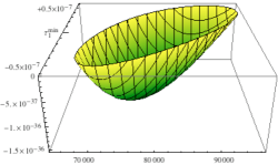
(a) $V_{F}(\mathcal{V},\tau_{1})$

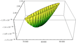
(b) $V_{F}(\mathcal{V},\tau_{2})$

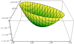
(c) $V_{F}(\tau_{1},\tau_{2})$

Figure 2: F-term potential of the GUT model 1 in the vicinity of the minimum.

The various masses are computed using the formulas from above. Let us however emphasise that for the gaugino and scalar masses it is crucial to work with precise values for $T_{1}^{*}$, $T_{2}^{*}$ and $\mathcal{V}^{*}$ in order to numerically obtain certain cancellations.

$$\begin{array}[]{@{\hspace{9pt}}lclll@{\hspace{9pt}}||@{\hspace{9pt}} lclll@{\hspace{9pt}}||@{\hspace{9pt}} lclll@{\hspace{9pt}}}\hskip 9.0pt\lx@intercol\hfil\mbox{Fundamental Masses}\hfil\hskip 9.0pt\vrule\vrule\hskip 9.0pt&\lx@intercol\hfil\mbox{Moduli Masses}\hfil\hskip 9.0pt\vrule\vrule\hskip 9.0pt&\lx@intercol\hfil\mbox{Soft Masses}\hfil\hskip 9.0pt\\ \hline\cr\hline\cr\hskip 9.0pt\lx@intercol M_{\rm s}&=&1.2\,\cdot&10^{16}&{\rm GeV}\hfil\hskip 9.0pt\vrule\vrule\hskip 9.0&M_{U}&=&3.1\,\cdot&10^{13}&{\rm GeV}\hfil\hskip 9.0pt\vrule\vrule\hskip 9.0&m_{1/2}^{\rm gravity}&=&1.1\,\cdot&10^{-5}&{\rm GeV}\hfil\hskip 9.0\\ \hskip 9.0pt\lx@intercol M_{3/2}&=&1.6\,\cdot&10^{4}&{\rm GeV}\hfil\hskip 9.0pt\vrule\vrule\hskip 9.0&M_{T_{1}}&=&1.2\,\cdot&10^{9}&{\rm GeV}\hfil\hskip 9.0pt\vrule\vrule\hskip 9.0&m_{1/2,\,\scriptscriptstyle SU(3)}^{\rm anomaly}&=&1.2\,\cdot&10^{-3}&{\rm GeV}\hfil\hskip 9.0\\ \hskip 9.0pt\lx@intercol&&&&\hfil\hskip 9.0pt\vrule\vrule\hskip 9.0&M_{T_{2}}&=&1.6\,\cdot&10^{4}&{\rm GeV}\hfil\hskip 9.0pt\vrule\vrule\hskip 9.0&m_{0}^{\rm gravity}&=&64&&{\rm GeV}\hfil\hskip 9.0\\ \hskip 9.0pt\lx@intercol&&&&\hfil\hskip 9.0pt\vrule\vrule\hskip 9.0&M_{T_{\rm b}}&=&56&&{\rm GeV}\hfil\hskip 9.0pt\vrule\vrule\hskip 9.0\end{array}$$

Let us comment on these scales:

• By construction, the string scale $M_{\rm s}$ coincides with the GUT scale and the gravitino mass $M_{3/2}$ is in the TeV regime.

• The closed sector moduli masses are ordered from heavy to light and take acceptable values except for $T_{\rm b}$ which is too small. For $M_{s}=M_{X}$, the lower bound for moduli masses not to be in conflict with cosmology is around $1\,{\rm TeV}$. Therefore, in this model we face the Cosmological Moduli Problem (CMP) [36, 37].

• In addition, the gaugino as well as the scalar masses are far too small. The main reason is that we realised the MSSM on the cycle $\Gamma_{1}$ which is related to the race-track modulus $T_{1}$. For this modulus we observe numerical cancellations giving $F^{1}\simeq 2\cdot 10^{-22}\,M_{\rm Pl}\sim 10^{-8}\,M_{3/2}$, i.e. supersymmetry breaking on the race-track cycle is eight orders of magnitude smaller than naively expected. The explanation is that the exact race-track minimum, in leading order given by the globally supersymmetric minimum (2.9), is almost supersymmetric. For the gravity mediated gaugino masses we therefore obtain a strong suppression

  $$\begin{split}m_{1/2}^{\rm gravity}=\frac{1}{2\,\tau_{1}}\>F^{1}\sim\frac{1}{2\cdot 25}\>2\cdot 10^{-22}\>M_{\rm Pl}\sim 10^{-5}\,{\rm GeV}\;.\end{split}$$ (3.10)

• For the anomaly mediated gaugino masses $m_{1/2}^{\rm anomaly}$, we find the expected cancellation of $M_{3/2}$ at leading order (see [35] for a detailed derivation), however the sub-leading order in $\mathcal{V}$ dominates over $F^{1}$

  $$\begin{split}m_{1/2,\,\scriptscriptstyle SU(3)}^{\rm anomaly}&\sim\frac{\alpha_{a}}{4\pi}\>\biggl{(}3\,T_{G}\,M_{3/2}\,\Bigl{(}1-1+\mathcal{O}\bigl{(}\mathcal{V}^{-1}\bigr{)}\Bigr{)}+2\,\lambda\,T_{R}\>\frac{F^{1}}{2\,\tau_{1}}\biggr{)}\\ &\sim\frac{1}{300}\>\biggl{(}3\cdot 3\cdot 10^{4}\,{\rm GeV}\cdot 10^{-5}+2\,\lambda\cdot 6\cdot\frac{2\cdot 10^{-22}\,M_{\rm Pl}}{2\cdot 25}\biggr{)}\\[3.0pt] &\sim 10^{-3}\,{\rm GeV}\;.\end{split}$$ (3.11)

  This value is of course still too small but note it is larger than the gravity mediated term. The gaugino masses are thus dominantly generated via anomaly mediation.

• A similar mechanism is at work for the scalar masses where $M_{3/2}^{2}$ is cancelled at leading order and subleading corrections in $\mathcal{V}$ give the main contribution (see again [35] for a detailed derivation of this expression)

  $$\begin{split}\bigl{(}m_{0}^{\rm gravity}\bigr{)}^{2}&\sim M_{3/2}^{2}\,\Bigl{(}1-1+\mathcal{O}\bigl{(}\mathcal{V}^{-1}\bigr{)}\Bigr{)}+\lambda\,\biggl{(}\frac{F^{1}}{2\,\tau_{1}}\biggr{)}^{2}\\ &\sim\bigl{(}10^{4}\,{\rm GeV}\bigr{)}^{2}\cdot 10^{-5}+\lambda\,\biggl{(}\frac{2\cdot 10^{-22}\,M_{\rm Pl}}{2\cdot 25}\biggr{)}^{2}\\[3.0pt] &\sim\bigl{(}10^{3/2}\,{\rm GeV}\bigr{)}^{2}\;.\end{split}$$ (3.12)

In conclusion, although we were able to easily arrange for $M_{\rm s}\simeq M_{X}$, $\alpha^{-1}\simeq\alpha^{-1}_{X}\simeq 25$ and a gravitino mass in the TeV range, the soft terms are much too small. In order to obtain realistic soft masses, two options seem viable. Either we take the present setup and scale the mass parameters by a factor of $10^{6}$, or we wrap the MSSM branes not only along $\Gamma_{1}$ but on $\Gamma_{1}+\Gamma_{2}$ giving also a contribution from $F^{2}$ to the soft terms. In the following two subsections, we discuss these two possibilities in more detail.

3.2 Model 2: A Mixed Anomaly-Gravity Mediated Model

Recall that the minimum for the race-track modulus $T_{1}$ is approximately supersymmetric. To construct a model with gaugino masses in the TeV range, we use the same set of parameters (3.8) of the previous setup but scale $\mathcal{A}$ and $\mathcal{B}$ to somewhat more unrealistic values

$$\begin{split}\mathcal{A}=1.6\;\times\;8\cdot 10^{5}\;,\qquad\mathcal{B}=0.2\;\times\;8\cdot 10^{5}\;.\end{split}$$ (3.13)

The minimum of the resulting F-term potential is not changed except for the value of $V_{F}$ in the minimum

$$\begin{split}\mathcal{V}^{*}=78559\;,\quad T_{1}^{*}=25.18\;,\quad T_{2}^{*}=2.88\;,\quad V_{F}^{*}=-9.5\cdot 10^{-25}\,M_{\rm Pl}^{4}\;.\end{split}$$ (3.14)

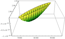
(b) $V_{F}(\mathcal{V},\tau_{2})$

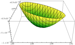
(c) $V_{F}(\tau_{1},\tau_{2})$

Figure 3: F-term potential of the GUT model 2 in the vicinity of the minimum.

Three plots showing the potential in the vicinity of the minimum can be found in figures 3 on page 3 and the mass scales for the new setup are the following:

$$\begin{array}[]{@{\hspace{9pt}}lclll@{\hspace{9pt}}||@{\hspace{9pt}} lclll@{\hspace{9pt}}||@{\hspace{9pt}} lclll@{\hspace{9pt}}}\hskip 9.0pt\lx@intercol\hfil\mbox{Fundamental Masses}\hfil\hskip 9.0pt\vrule\vrule\hskip 9.0pt&\lx@intercol\hfil\mbox{Moduli Masses}\hfil\hskip 9.0pt\vrule\vrule\hskip 9.0pt&\lx@intercol\hfil\mbox{Soft Masses}\hfil\hskip 9.0pt\\ \hline\cr\hline\cr\hskip 9.0pt\lx@intercol M_{\rm s}&=&1.2\,\cdot&10^{16}&{\rm GeV}\hfil\hskip 9.0pt\vrule\vrule\hskip 9.0&M_{U}&=&3.1\,\cdot&10^{13}&{\rm GeV}\hfil\hskip 9.0pt\vrule\vrule\hskip 9.0&m_{1/2}^{\rm gravity}&=&8.6&&{\rm GeV}\hfil\hskip 9.0\\ \hskip 9.0pt\lx@intercol M_{3/2}&=&1.3\,\cdot&10^{10}&{\rm GeV}\hfil\hskip 9.0pt\vrule\vrule\hskip 9.0&M_{T_{1}}&=&9.9\,\cdot&10^{14}&{\rm GeV}\hfil\hskip 9.0pt\vrule\vrule\hskip 9.0&m_{1/2,\,\scriptscriptstyle SU(3)}^{\rm anomaly}&=&962&&{\rm GeV}\hfil\hskip 9.0\\ \hskip 9.0pt\lx@intercol&&&&\hfil\hskip 9.0pt\vrule\vrule\hskip 9.0&M_{T_{2}}&=&1.3\,\cdot&10^{10}&{\rm GeV}\hfil\hskip 9.0pt\vrule\vrule\hskip 9.0&m_{0}^{\rm gravity}&=&5.1\,\cdot&10^{7}&{\rm GeV}\hfil\hskip 9.0\\ \hskip 9.0pt\lx@intercol&&&&\hfil\hskip 9.0pt\vrule\vrule\hskip 9.0&M_{T_{\rm b}}&=&4.5\,\cdot&10^{7}&{\rm GeV}\hfil\hskip 9.0pt\vrule\vrule\hskip 9.0\end{array}$$

We again comment on these scales:

• Since the value of the volume modulus is not changed compared to the previous setup, we similarly obtain $M_{\rm s}\simeq M_{X}$. However, the gravitino mass is in an intermediate regime due to the change in $W_{0}^{\rm eff}$.

• With the gravitino masses in the intermediate regime, the Cosmological Moduli Problem has been evaded, as $T_{\rm b}$ is much heavier then the TeV scale. We also see that $M_{T_{1}}>M_{U}$, but since we have a well-defined expansion in $1/\mathcal{V}$ we can safely stabilise $U$ and then study the stabilisation of $T_{1}$.

• Concerning the gravity mediated gaugino mass, the scaling (3.13) results in a value of $W_{0}^{\rm eff}$ which is $8\cdot 10^{5}$ times larger than in the previous setup leading to $F^{1}\sim 10^{-16}\,M_{\rm Pl}$. The gravity mediated gaugino mass $m_{1/2}^{\rm gravity}$ is still too small but the anomaly mediated masses are now in the TeV regime.

• As expected from the first example, the gravity mediated scalar masses are at $m^{\rm gravity}_{0}\sim 10^{7}\,{\rm GeV}$ and therefore much heavier than the gaugino masses. However, they come in complete $SU(5)$ multiplets and therefore do not spoil gauge coupling unification.

• With this hierarchy between the gaugino masses and the scalar masses, we have a dynamical realisation of the split supersymmetry scenario [38]. The Higgs sector masses, i.e. the canonically normalised $\hat{\mu}$-term and the soft term $\mu B$, are expected to be of the same order of magnitude as the scalar masses, simply for the reason that here both $F^{\rm b}\sim M_{3/2}$ and $F^{1}$ contribute. Therefore, in order to keep these at the weak scale, a fine-tuning of the supersymmetric $\mu$-term is necessary.

To summarise, tuning the initial parameters such that $\alpha^{-1}\simeq\alpha_{X}^{-1}\simeq 25$ and $M_{s}=M_{X}$, and localising the MSSM solely on the race-track cycle $\Gamma_{1}$, we find a high suppression of the gravity mediated gaugino masses due to the quasi-supersymmetry of the race-track minimum. Fixing the gaugino masses at the TeV scale leads to an intermediate supersymmetry breaking scenario with gravitino masses and scalar masses in the intermediate regime. Due to the large value of $M_{3/2}$, this evades the CMP and gives a stringy realisation of the split supersymmetry scenario proposed in [38].

3.3 Model 3: An LVS like Supergravity Mediated Model

We now consider the second possibility from the end of section 3.1 which indeed realises our initial goal, namely to naturally find large volume minima with the string scale at the GUT scale, gauge coupling unification and soft masses in the TeV regime. This provides a concrete moduli stabilisation scenario for which the analysis of [41] is applicable. There, the computation of soft masses and running to the weak scale has been studied quite systematically for moduli dominated supersymmetry breaking in F-theory respectively Type IIB orientifold compactifications realising the MSSM.

We modify our original setup such that the soft terms are dominantly generated via $T_{2}$ similarly to the original LVS. To do so, we place the MSSM $D7$-branes on the combination of cycles $\Gamma_{1}+\Gamma_{2}$. A concrete set of parameters realising this setup without fine-tuning is

$$\begin{array}[]{@{}lcllcllcllcllcllcl@{}}\mathcal{A}&=&1.5\,,&\mathcal{B}&=&0.25\,,&\mathcal{C}_{1}&=&1\,,&\mathcal{C}_{2}&=&3\,,&a&=&\frac{2\pi}{8}\,,&b&=&\frac{2\pi}{9}\,,\\[4.0pt] g_{s}&=&\frac{2}{5}\,,&\eta_{\rm b}&=&1\,,&\eta_{1}&=&\frac{1}{40}\,,&\eta_{2}&=&\frac{1}{6}\,,&\chi&=&\lx@intercol-153\,.\hfil\lx@intercol\end{array}$$ (3.15)

The minimum of the scalar F-term potential is again determined with the help of Mathematica giving

$$\begin{split}\mathcal{V}^{*}=92158\;,\quad T_{1}^{*}=21.58\;,\quad T_{2}^{*}=2.91\;,\quad V_{F}^{*}=-1.4\cdot 10^{-34}\,M_{\rm Pl}^{4}\;,\end{split}$$ (3.16)

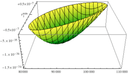
(a) $V_{F}(\mathcal{V},\tau_{1})$

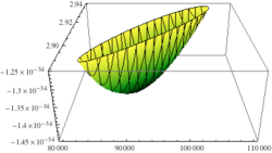
(b) $V_{F}(\mathcal{V},\tau_{2})$

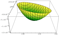
(c) $V_{F}(\tau_{1},\tau_{2})$

Figure 4: F-term potential of the GUT model 3 in the vicinity of the minimum.

so that the gauge coupling of the D7-branes $\alpha^{-1}=\tau_{1}+\tau_{2}=24.8$ is again the unified gauge coupling at the GUT scale. Three plots showing the potential in the vicinity of the minimum can be found in figures 4 on page 4. The mass scales in this setup are calculated as follows:

$$\begin{array}[]{@{\hspace{9pt}}lclll@{\hspace{9pt}}||@{\hspace{9pt}} lclll@{\hspace{9pt}}||@{\hspace{9pt}} lclll@{\hspace{9pt}}}\hskip 9.0pt\lx@intercol\hfil\mbox{Fundamental Masses}\hfil\hskip 9.0pt\vrule\vrule\hskip 9.0pt&\lx@intercol\hfil\mbox{Moduli Masses}\hfil\hskip 9.0pt\vrule\vrule\hskip 9.0pt&\lx@intercol\hfil\mbox{Soft Masses}\hfil\hskip 9.0pt\\ \hline\cr\hline\cr\hskip 9.0pt\lx@intercol M_{\rm s}&=&1.1\,\cdot&10^{16}&{\rm GeV}\hfil\hskip 9.0pt\vrule\vrule\hskip 9.0&M_{U}&=&2.6\,\cdot&10^{13}&{\rm GeV}\hfil\hskip 9.0pt\vrule\vrule\hskip 9.0&m_{1/2}^{\rm gravity}&=&819&&{\rm GeV}\hfil\hskip 9.0\\ \hskip 9.0pt\lx@intercol M_{3/2}&=&168&&{\rm TeV}\hfil\hskip 9.0pt\vrule\vrule\hskip 9.0&M_{T_{1}}&=&1.5\,\cdot&10^{10}&{\rm GeV}\hfil\hskip 9.0pt\vrule\vrule\hskip 9.0&m_{1/2,\,\scriptscriptstyle SU(3)}^{\rm anomaly}&=&10&&{\rm GeV}\hfil\hskip 9.0\\ \hskip 9.0pt\lx@intercol&&&&\hfil\hskip 9.0pt\vrule\vrule\hskip 9.0&M_{T_{2}}&=&168&&{\rm TeV}\hfil\hskip 9.0pt\vrule\vrule\hskip 9.0&m_{0}^{\rm gravity}&=&817&&{\rm GeV}\hfil\hskip 9.0\\ \hskip 9.0pt\lx@intercol&&&&\hfil\hskip 9.0pt\vrule\vrule\hskip 9.0&M_{T_{\rm b}}&=&553&&{\rm GeV}\hfil\hskip 9.0pt\vrule\vrule\hskip 9.0\end{array}$$

Let us again comment on the various scales arising in this large volume minimum:

• We arranged the parameters for the present setup such that $M_{\rm s}\simeq M_{X}$ together with the gravitino mass in the TeV range.

• The closed sector moduli masses take (almost) acceptable values with $M_{T_{\rm b}}$ close to the regime where the Cosmological Moduli Problem may be avoided. (Note that we were not careful with factors of $2\pi$.)

• The soft masses are dominantly generated via the supersymmetry breaking of $T_{2}$ specified by $F^{2}\sim 10^{-14}M_{\rm Pl}$. Since $T_{2}$ is stabilised as in the original LARGE Volume Scenario, similar mechanisms generating the soft masses are at work [35]. In particular, using the fact that $F^{1}\sim 10^{-20}M_{\rm Pl}\ll F^{2}$, the common term determining the gaugino as well as the scalar masses can be expressed as

  $$\begin{split}\frac{F^{1}+F^{2}}{2\,\bigl{(}\tau_{1}+\tau_{2}\bigr{)}}\sim\frac{F^{2}}{2\,\bigl{(}\tau_{1}+\tau_{2}\bigr{)}}\sim\frac{\tau_{2}}{\tau_{1}+\tau_{2}}\>\frac{M_{3/2}}{\ln\left(M_{\rm Pl}/M_{3/2}\right)}\;.\end{split}$$ (3.17)

  Here we used that $F^{2}\simeq 2\tau_{2}\,M_{3/2}/\ln\left(M_{\rm Pl}/M_{3/2}\right)$ which was obtained in [42]. For the gravity mediated gaugino mass we thus find

  $$\begin{split}m_{1/2}^{\rm gravity}=\frac{F^{1}+F^{2}}{2\,\bigl{(}\tau_{1}+\tau_{2}\bigr{)}}\>\sim\frac{3}{25}\>\frac{1.7\cdot 10^{5}\,{\rm GeV}}{\ln\bigl{(}10^{18}\cdot 10^{-5}\bigr{)}}\sim 700\,{\rm GeV}\;.\end{split}$$ (3.18)

• For the anomaly mediated gaugino mass we use equation (3.11) to obtain

  $$m_{1/2,\,\scriptscriptstyle SU(3)}^{\rm anomaly} \sim\frac{\alpha_{a}}{4\pi}\>\biggl{(}3\,T_{G}\,M_{3/2}\,\Bigl{(}1-1+\mathcal{O}\bigl{(}\mathcal{V}^{-1}\bigr{)}\Bigr{)}+2\,\lambda\,T_{R}\>\frac{F^{1}+F^{2}}{2\,\bigl{(}\tau_{1}+\tau_{2}\bigr{)}}\biggr{)}$$

  $$\sim\frac{1}{300}\>\biggl{(}3\cdot 3\cdot 10^{5}\,{\rm GeV}\cdot 10^{-6}+2\,\lambda\cdot 6\cdot 700\,{\rm GeV}\biggr{)}$$ (3.19)

  $$\sim 10\,{\rm GeV}\;,$$

  with $\lambda=1/3$ [35]. Note that again the contribution of $M_{3/2}$ is cancelled at leading order but the subleading correction $M_{3/2}/\mathcal{V}$ is suppressed compared to $F^{2}$.

  Furthermore, in this supersymmetry breaking scheme, the anomaly mediated gaugino masses are significantly smaller than the gravity mediated ones. This is contrast to the so-called mirage mediation scheme arising for instance in the original KKLT scenario [43, 44, 45], where both are of the same order of magnitude.

• Finally, we consider the gravity mediated scalar masses. Referring to formula (3.12), we obtain

  $$\begin{split}\bigl{(}m_{0}^{\rm gravity}\bigr{)}^{2}&\sim M_{3/2}^{2}\,\Bigl{(}1-1+\mathcal{O}\bigl{(}\mathcal{V}^{-1}\bigr{)}\Bigr{)}+\lambda\,\biggl{(}\frac{F^{1}+F^{2}}{2\,\bigl{(}\tau_{1}+\tau_{2}\bigr{)}}\biggr{)}^{2}\\[3.0pt] &\sim\bigl{(}10^{5}\,{\rm GeV}\bigr{)}^{2}\cdot 10^{-6}+\lambda\,\bigl{(}700\,{\rm GeV}\bigr{)}^{2}\\[4.0pt] &\sim\bigl{(}10^{2}\,{\rm GeV}\bigr{)}^{2}\;.\end{split}$$ (3.20)

  Note that for the scalar masses, the contribution from $M_{3/2}$ is cancelled at leading order but now the subleading corrections scale as $M_{3/2}/\sqrt{\mathcal{V}}$. Therefore, by accident, the two terms in the equation above are of the same order which is in contrast to the relation $m_{0}^{\rm gravity}=m_{1/2}^{\rm gravity}/\sqrt{3}$ obtained in the LVS [35].

• Assuming that the supersymmetric $\mu$-term vanishes, the canonical normalised Higgs parameters are also in the TeV regime. This would solve the $\mu$-problem via the Giudice-Masiero mechanism [46].

In summary, by wrapping the MSSM supporting $D7$-branes along $\Gamma_{1}+\Gamma_{2}$, we obtain a LARGE Volume Scenario with supergravity mediated soft masses in the TeV region and $M_{\rm s}=M_{X}$. This is different compared to the original LVS where the string scale is usually at an intermediate scale. Along the lines of [9, 41], the next step is to calculate the soft-terms at the weak scale to see whether distinctive patterns for the supersymmetric phenomenology to be tested at the LHC can be obtained.

4 Comment on the Cosmological Constant

For the GUT setup discussed in the previous section, the tree-level cosmological constant is $V_{F}^{*}=-1.4\cdot 10^{-34}M_{\rm Pl}^{4}$ and therefore a high degree of fine-tuning in the uplift potential (2.13) is needed to obtain $\Lambda\simeq+10^{-120}\,M_{\rm Pl}^{4}$. After such a fine-tuning has been achieved, a LARGE volume scenario with $M_{\rm s}\simeq M_{X}$ contains a natural candidate serving as a quintessence field [47, 48, 49]. Indeed, taking into account also non-perturbative corrections corresponding to the large four-cycle $\Gamma_{\rm b}$, the scalar potential depending on the (canonically normalised) axion $\sigma_{\rm b}$ takes the form

$$\begin{split}\frac{V_{Q}}{M_{\rm Pl}^{4}}\simeq\left(\frac{M_{\rm Pl}\,M_{3/2}}{M_{X}^{2}}\right)\,\>e^{-\frac{2\pi}{L}\tau_{\rm b}}\>\biggl{(}1-\cos\biggl{(}\frac{2\pi}{L}\,\sigma_{\rm b}\biggr{)}\biggr{)}\;.\end{split}$$ (4.1)

For the minimum $\mathcal{V}^{*}\simeq\tau_{\rm b}^{2/3}\simeq 92158$ of our model from section 3.3 and $L$ of the order $L=40\ldots 50$, the prefactor in (4.1) is of the right order of magnitude.

Although the GUT models from the previous section may contain a quintessence field, let us now take a different point of view. Since in our scenario we have exponential control over $W_{0}^{\rm eff}$ and $A^{\rm eff}$, one might ask whether it is possible to dynamically find a minimum $V_{F}^{*}\simeq-\lvert W^{\rm eff}_{0}\rvert^{2}\,\mathcal{V}^{-3}\simeq-10^{-120}M_{\rm Pl}^{4}$ realised without fine-tuning. Ignoring the weak scale for a moment, for the string scale we have $M_{\rm s}\sim\mathcal{V}^{-1/2}M_{\rm Pl}>{\rm TeV}$ which implies that $\mathcal{V}<10^{30}$. To keep the tuning of $a,b,\mathcal{A},\mathcal{B}$ moderate, we identify $\lvert W_{0}^{\rm eff}\rvert\sim 10^{-15}$ and thus $\mathcal{V}\sim 10^{30}$ as a natural choice to realise $V_{F}^{*}\simeq-10^{-120}M_{\rm Pl}^{4}$. A set of parameters dynamically leading to such values is for instance

$$\begin{array}[]{@{}lcllcllcllcllcllcl@{}}\mathcal{A}&=&1\,,&\mathcal{B}&=&0.1\,,&\mathcal{C}_{1}&=&1\,,&\mathcal{C}_{2}&=&3\,,&a&=&\frac{2\pi}{13}\,,&b&=&\frac{2\pi}{14}\,,\\[4.0pt] g_{s}&=&\frac{1}{5}\,,&\eta_{\rm b}&=&1\,,&\eta_{1}&=&\frac{1}{30}\,,&\eta_{2}&=&\frac{1}{6}\,,&\chi&=&\lx@intercol-452\,,\hfil\lx@intercol\end{array}$$

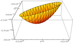
(b) $V_{F}(\mathcal{V},\tau_{2})$

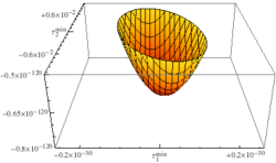
(c) $V_{F}(\tau_{1},\tau_{2})$

Figure 5: F-term potential of the $\Lambda$ model in the vicinity of the minimum.

and the plots showing the potential in the vicinity of the minimum can be found in figures 5 on page 5. The numerical values specifying the minimum are

$$\begin{split}\mathcal{V}^{*}=6.4\cdot 10^{28}\;,\quad T_{1}^{*}=68.84\;,\quad T_{2}^{*}=11.53\;,\quad V_{F}^{*}=-7.8\cdot 10^{-121}M_{\rm Pl}^{4}\;,\end{split}$$ (4.2)

and because the AdS minimum is at $V_{F}^{*}\sim-10^{-120}M_{\rm Pl}^{4}$, the warp factor $a=10^{-15}$ in the uplift potential (2.13) does not involve any fine-tuning of the flux parameters $K$ and $M$.

We conclude that there exist vacua of the scalar potential (2) whose tree-level cosmological constant has the right order of magnitude. However, this clearly does not solve the cosmological constant problem, as we have not yet identified the Standard Model and the origin of the weak scale. Once we try to introduce the MSSM into this set-up, we are confronted with the usual problems. Let us briefly explain three possibilities:

• Localising the MSSM on $D7$-branes wrapping the cycles $\Gamma_{(1,2)}$ leads to soft masses below the gravitino mass scale $M_{3/2}\simeq 10^{-18}\,{\rm eV}$ which itself is ridiculously small.

• Since $M_{\rm s}\sim{\rm TeV}$, we could break supersymmetry at the string scale and place a non-supersymmetric anti $D3$-brane configuration realising the MSSM at the bottom of a throat, i.e. on the TeV brane in the RS scenario. The uncancelled NS-NS tadpole of the non-supersymmetric brane configuration would be the red-shifted uplift term. However, all mass scales in the throat are red-shifted as well [4] so that the stringy excitations such as squarks have masses $M_{\tilde{Q}}\simeq a\,M_{\rm s}\simeq\Lambda^{1/4}=10^{-3}\,{\rm eV}$.

• A third option is to place an explicitly supersymmetry breaking D-brane configuration in the bulk, i.e. on the Planck brane in the RS scenario. Then the superpartners have string scale masses in the TeV region, but we get an additional positive contribution $V\sim\mathcal{O}(M_{\rm s}^{4})$ to the scalar potential.

In conclusion, even though we have exponential control over the effective parameters $W_{0}^{\rm eff}$ and $A^{\rm eff}$, the cosmological constant problem is not even touched. It can be phrased as the problem of hiding the TeV scale supersymmetry breaking of the Standard Model such that it does not induce a large contribution to the tree-level value $\Lambda_{0}$.

5 Summary and Conclusions

In this paper, we have studied string theory compactifications of type IIB orientifolds where the complex structure moduli are assumend to be stabilised by fluxes such that $W_{\rm flux}\rvert_{\rm min.}=0$. In addition, we considered a compactification manifold of swiss-cheese type where gaugino condensation on two stacks of $D7$-branes leads to a race-track superpotential. Taking into account instanton corrections to the gauge kinetic function manifesting themselves as poly-instanton corrections to the race-track superpotential, we constructed a scenario featuring exponential control over the parameters $W_{0}^{\rm eff}$ and $A^{\rm eff}$ in an effective superpotential of the form $W^{\rm eff}=W_{0}^{\rm eff}-A^{\rm eff}\exp(-a\,T)$. Such superpotentials are used for moduli stabilisation in KKLT and LARGE Volume Scenarios. However, in our setup we can arrange for exponential small values of these parameters without fine-tuning.

Using this setup, we were able to find minima of the resulting scalar potential realising supersymmetric GUT scenarios featuring $M_{\rm s}=M_{X}\simeq 1.2\cdot 10^{16}\,{\rm GeV}$, $\alpha^{-1}\simeq\alpha^{-1}_{X}\simeq 25$ and a gravitino mass in the TeV region without fine-tuning. However, despite the phenomenological interesting value of $M_{3/2}$, the soft terms in our first setup are strongly suppressed. The reason is that the race-track modulus is stabilised in a nearly supersymmetric minimum giving F-terms which are much smaller than expected. We proposed two resolutions of this issue and constructed the corresponding setups:

• First, we scaled our parameters such that effectively $W_{0}^{\rm eff}$ is scaled by a factor of $10^{6}$ leading to a larger gravitino mass but also to larger soft masses. The gaugino masses are dominantly generated by anomaly-mediation while the scalar masses are generated by gravity mediation leading to a stringy realisation of split supersymmetry if the Higgs and Higgsino masses are tuned to small values.

• The second possibility we considered was to generate the soft terms not by the F-term of the race-track modulus but also by the F-term of the small LVS Kähler modulus. The gaugino as well as the scalar masses are then generated by gravity mediation similarly to the original LARGE Volume Scenario. The lightest modulus was on the edge of posing problems with cosmology (CMP) and the $\mu$-problem could be solved by the Giudice-Masiero mechanism.

Clearly, a more detailed analysis of the phenomenological implications of these setups along the lines of [9, 41] would be very interesting. Moreover, it remains to be seen whether one can indeed construct global string or F-theory compactifications realising all the features we assumed for this scenario. Not the least challenge is to concretely evade the problem of intrinsic tension between moduli stabilisation via instantons and a chiral MSSM sector raised in [29].

Finally, in the last section we mentioned that for our GUT models there is, similarly to the LARGE Volume Scenarios, a natural candidate for a quintessence field. Taking a different point of view, we were also able to construct a setup with tree-level cosmological constant at the order of $\Lambda_{0}\sim-10^{-120}M^{4}_{\rm Pl}$ which can be uplifted to a positive value without fine-tuning. However, although we obtained an encouraging value for $\Lambda_{0}$, introducing the Standard Model in this setup will spoil this feature.

Acknowledgements

We gratefully acknowledge discussions with N. Akerblom, E. Dudas, T. Grimm, D. Lüst, M. Schmidt-Sommerfeld and T. Weigand. We also thank S. P. de Alwis for pointing out a possible unclarity in the first version of this paper.

(a) $V_{F}(\mathcal{V},\tau_{1})$

(a) $V_{F}(\mathcal{V},\tau_{1})$

References

- [1] N. Arkani-Hamed, S. Dimopoulos, and G. R. Dvali, “The hierarchy problem and new dimensions at a millimeter,” Phys. Lett. B429 (1998) 263–272, hep-ph/9803315.
- [2] I. Antoniadis, N. Arkani-Hamed, S. Dimopoulos, and G. R. Dvali, “New dimensions at a millimeter to a Fermi and superstrings at a TeV,” Phys. Lett. B436 (1998) 257–263, hep-ph/9804398.
- [3] I. Antoniadis, “A Possible new dimension at a few TeV,” Phys. Lett. B246 (1990) 377–384.
- [4] L. Randall and R. Sundrum, “A large mass hierarchy from a small extra dimension,” Phys. Rev. Lett. 83 (1999) 3370–3373, hep-ph/9905221.
- [5] S. Kachru, R. Kallosh, A. Linde, and S. P. Trivedi, “De Sitter vacua in string theory,” Phys. Rev. D68 (2003) 046005, hep-th/0301240.
- [6] V. Balasubramanian, P. Berglund, J. P. Conlon, and F. Quevedo, “Systematics of moduli stabilisation in Calabi-Yau flux compactifications,” JHEP 03 (2005) 007, hep-th/0502058.
- [7] M. Cicoli, J. P. Conlon, and F. Quevedo, “General Analysis of LARGE Volume Scenarios with String Loop Moduli Stabilisation,” 0805.1029.
- [8] J. P. Conlon, F. Quevedo, and K. Suruliz, “Large-volume flux compactifications: Moduli spectrum and D3/D7 soft supersymmetry breaking,” JHEP 08 (2005) 007, hep-th/0505076.
- [9] J. P. Conlon, C. H. Kom, K. Suruliz, B. C. Allanach, and F. Quevedo, “Sparticle Spectra and LHC Signatures for Large Volume String Compactifications,” JHEP 08 (2007) 061, 0704.3403.
- [10] R. Blumenhagen and M. Schmidt-Sommerfeld, “Power Towers of String Instantons for N=1 Vacua,” 0803.1562.
- [11] B. S. Acharya, K. Bobkov, G. L. Kane, P. Kumar, and J. Shao, “Explaining the electroweak scale and stabilizing moduli in M theory,” Phys. Rev. D76 (2007) 126010, hep-th/0701034.
- [12] S. Gukov, C. Vafa, and E. Witten, “CFT’s from Calabi-Yau four-folds,” Nucl. Phys. B584 (2000) 69–108, hep-th/9906070.
- [13] O. DeWolfe, A. Giryavets, S. Kachru, and W. Taylor, “Enumerating flux vacua with enhanced symmetries,” JHEP 02 (2005) 037, hep-th/0411061.
- [14] K. Becker, M. Becker, M. Haack, and J. Louis, “Supersymmetry breaking and alpha’-corrections to flux induced potentials,” JHEP 06 (2002) 060, hep-th/0204254.
- [15] P. G. Camara, E. Dudas, T. Maillard, and G. Pradisi, “String instantons, fluxes and moduli stabilization,” Nucl. Phys. B795 (2008) 453–489, 0710.3080.
- [16] M. Billo et al., “Classical gauge instantons from open strings,” JHEP 02 (2003) 045, hep-th/0211250.
- [17] R. Blumenhagen, M. Cvetič, and T. Weigand, “Spacetime instanton corrections in 4D string vacua - the seesaw mechanism for D-brane models,” Nucl. Phys. B771 (2007) 113–142, hep-th/0609191.
- [18] L. E. Ibanez and A. M. Uranga, “Neutrino Majorana masses from string theory instanton effects,” JHEP 03 (2007) 052, hep-th/0609213.
- [19] B. Florea, S. Kachru, J. McGreevy, and N. Saulina, “Stringy instantons and quiver gauge theories,” JHEP 05 (2007) 024, hep-th/0610003.
- [20] N. Akerblom, R. Blumenhagen, D. Lüst, E. Plauschinn, and M. Schmidt-Sommerfeld, “Non-perturbative SQCD Superpotentials from String Instantons,” JHEP 04 (2007) 076, hep-th/0612132.
- [21] M. Bianchi and E. Kiritsis, “Non-perturbative and Flux superpotentials for Type I strings on the orbifold,” Nucl. Phys. B782 (2007) 26–50, hep-th/0702015.
- [22] M. Cvetič, R. Richter, and T. Weigand, “Computation of D-brane instanton induced superpotential couplings - Majorana masses from string theory,” Phys. Rev. D76 (2007) 086002, hep-th/0703028.
- [23] R. Argurio, M. Bertolini, G. Ferretti, A. Lerda, and C. Petersson, “Stringy Instantons at Orbifold Singularities,” JHEP 06 (2007) 067, 0704.0262.
- [24] M. Bianchi, F. Fucito, and J. F. Morales, “D-brane Instantons on the orientifold,” JHEP 07 (2007) 038, 0704.0784.
- [25] L. E. Ibanez, A. N. Schellekens, and A. M. Uranga, “Instanton Induced Neutrino Majorana Masses in CFT Orientifolds with MSSM-like spectra,” JHEP 06 (2007) 011, 0704.1079.
- [26] N. Akerblom, R. Blumenhagen, D. Lüst, and M. Schmidt-Sommerfeld, “Instantons and Holomorphic Couplings in Intersecting D- brane Models,” JHEP 08 (2007) 044, 0705.2366.
- [27] T. W. Grimm, “Non-Perturbative Corrections and Modularity in N=1 Type IIB Compactifications,” JHEP 10 (2007) 004, 0705.3253.
- [28] I. R. Klebanov and M. J. Strassler, “Supergravity and a confining gauge theory: Duality cascades and chiSB-resolution of naked singularities,” JHEP 08 (2000) 052, hep-th/0007191.
- [29] R. Blumenhagen, S. Moster, and E. Plauschinn, “Moduli Stabilisation versus Chirality for MSSM like Type IIB Orientifolds,” JHEP 01 (2008) 058, 0711.3389.
- [30] M. Berg, M. Haack, and E. Pajer, “Jumping Through Loops: On Soft Terms from Large Volume Compactifications,” JHEP 09 (2007) 031, 0704.0737.
- [31] K. Choi, A. Falkowski, H. P. Nilles, and M. Olechowski, “Soft supersymmetry breaking in KKLT flux compactification,” Nucl. Phys. B718 (2005) 113–133, hep-th/0503216.
- [32] L. Randall and R. Sundrum, “Out of this world supersymmetry breaking,” Nucl. Phys. B557 (1999) 79–118, hep-th/9810155.
- [33] J. A. Bagger, T. Moroi, and E. Poppitz, “Anomaly mediation in supergravity theories,” JHEP 04 (2000) 009, hep-th/9911029.
- [34] J. P. Conlon, D. Cremades, and F. Quevedo, “Kaehler potentials of chiral matter fields for Calabi-Yau string compactifications,” JHEP 01 (2007) 022, hep-th/0609180.
- [35] J. P. Conlon, S. S. Abdussalam, F. Quevedo, and K. Suruliz, “Soft SUSY breaking terms for chiral matter in IIB string compactifications,” JHEP 01 (2007) 032, hep-th/0610129.
- [36] T. Banks, D. B. Kaplan, and A. E. Nelson, “Cosmological implications of dynamical supersymmetry breaking,” Phys. Rev. D49 (1994) 779–787, hep-ph/9308292.
- [37] B. de Carlos, J. A. Casas, F. Quevedo, and E. Roulet, “Model independent properties and cosmological implications of the dilaton and moduli sectors of 4-d strings,” Phys. Lett. B318 (1993) 447–456, hep-ph/9308325.
- [38] N. Arkani-Hamed and S. Dimopoulos, “Supersymmetric unification without low energy supersymmetry and signatures for fine-tuning at the LHC,” JHEP 06 (2005) 073, hep-th/0405159.
- [39] I. Antoniadis and S. Dimopoulos, “Splitting supersymmetry in string theory,” Nucl. Phys. B715 (2005) 120–140, hep-th/0411032.
- [40] E. Dudas and S. K. Vempati, “Large D-terms, hierarchical soft spectra and moduli stabilisation,” Nucl. Phys. B727 (2005) 139–162, hep-th/0506172.
- [41] L. Aparicio, D. G. Cerdeno, and L. E. Ibanez, “Modulus-dominated SUSY-breaking soft terms in F-theory and their test at LHC,” 0805.2943.
- [42] J. P. Conlon and F. Quevedo, “Gaugino and scalar masses in the landscape,” JHEP 06 (2006) 029, hep-th/0605141.
- [43] M. Endo, M. Yamaguchi, and K. Yoshioka, “A bottom-up approach to moduli dynamics in heavy gravitino scenario: Superpotential, soft terms and sparticle mass spectrum,” Phys. Rev. D72 (2005) 015004, hep-ph/0504036.
- [44] K. Choi, K. S. Jeong, and K.-i. Okumura, “Phenomenology of mixed modulus-anomaly mediation in fluxed string compactifications and brane models,” JHEP 09 (2005) 039, hep-ph/0504037.
- [45] K. Choi and H. P. Nilles, “The gaugino code,” JHEP 04 (2007) 006, hep-ph/0702146.
- [46] G. F. Giudice and A. Masiero, “A Natural Solution to the mu Problem in Supergravity Theories,” Phys. Lett. B206 (1988) 480–484.
- [47] K. Choi, “String or M theory axion as a quintessence,” Phys. Rev. D62 (2000) 043509, hep-ph/9902292.
- [48] P. Svrcek, “Cosmological constant and axions in string theory,” hep-th/0607086.
- [49] F. Quevedo, “LARGE volume string scenarios (talk at the String Phenomenology Conference 2008 in Philadelphia),” http://www.math.upenn.edu/StringPhenom2008/.