Manifold Learning: The Price of Normalization

Abstract

We analyze the performance of a class of manifold-learning algorithms that find their output by minimizing a quadratic form under some normalization constraints. This class consists of Locally Linear Embedding (LLE), Laplacian Eigenmap, Local Tangent Space Alignment (LTSA), Hessian Eigenmaps (HLLE), and Diffusion maps. We present and prove conditions on the manifold that are necessary for the success of the algorithms. Both the finite sample case and the limit case are analyzed. We show that there are simple manifolds in which the necessary conditions are violated, and hence the algorithms cannot recover the underlying manifolds. Finally, we present numerical results that demonstrate our claims.

Keywords: dimensionality reduction, manifold learning, Laplacian eigenmap, diffusion maps, locally linear embedding, local tangent space alignment,hessian eigenmap

1 Introduction

Many seemingly complex systems described by high-dimensional data sets are in fact governed by a surprisingly low number of parameters. Revealing the low-dimensional representation of such high-dimensional data sets not only leads to a more compact description of the data, but also enhances our understanding of the system. Dimension-reducing algorithms attempt to simplify the system’s representation without losing significant structural information. Various dimension-reduction algorithms were developed recently to perform embeddings for manifold-based data sets. These include the following algorithms: Locally Linear Embedding (LLE, Roweis and Saul, 2000), Isomap (Tenenbaum et al., 2000), Laplacian Eigenmaps (LEM, Belkin and Niyogi, 2003), Local Tangent Space Alignment (LTSA, Zhang and Zha, 2004), Hessian Eigenmap (HLLE, Donoho and Grimes, 2004), Semi-definite Embedding (SDE, Weinberger and Saul, 2006) and Diffusion Maps (DFM, Coifman and Lafon, 2006).

These manifold-learning algorithms compute an embedding for some given input. It is assumed that this input lies on a low-dimensional manifold, embedded in some high-dimensional space. Here a manifold is defined as a topological space that is locally equivalent to a Euclidean space. It is further assumed that the manifold is the image of a low-dimensional domain. In particular, the input points are the image of a sample taken from the domain. The goal of the manifold-learning algorithms is to recover the original domain structure, up to some scaling and rotation. The non-linearity of these algorithms allows them to reveal the domain structure even when the manifold is not linearly embedded.

The central question that arises when considering the output of a manifold-learning algorithm is, whether the algorithm reveals the underlying low-dimensional structure of the manifold. The answer to this question is not simple. First, one should define what “revealing the underlying lower-dimensional description of the manifold” actually means. Ideally, one could measure the degree of similarity between the output and the original sample. However, the original low-dimensional data representation is usually unknown. Nevertheless, if the low-dimensional structure of the data is known in advance, one would expect it to be approximated by the dimension-reducing algorithm, at least up to some rotation, translation, and global scaling factor. Furthermore, it would be reasonable to expect the algorithm to succeed in recovering the original sample’s structure asymptotically, namely, when the number of input points tends to infinity. Finally, one would hope that the algorithm would be robust in the presence of noise.

Previous papers have addressed the central question posed earlier. Zhang and Zha (2004) presented some bounds on the local-neighborhoods’ error-estimation for LTSA. However, their analysis says nothing about the global embedding. Huo and Smith (2006) proved that, asymptotically, LTSA recovers the original sample up to an affine transformation. They assume in their analysis that the level of noise tends to zero when the number of input points tends to infinity. Bernstein et al. (2000.) proved that, asymptotically, the embedding given by the Isomap algorithm (Tenenbaum et al., 2000) recovers the geodesic distances between points on the manifold.

In this paper we develop theoretical results regarding the performance of a class of manifold-learning algorithms, which includes the following five algorithms: Locally Linear Embedding (LLE), Laplacian Eigenmap (LEM), Local Tangent Space Alignment (LTSA), Hessian Eigenmaps (HLLE), and Diffusion maps (DFM).

We refer to this class of algorithms as the normalized-output algorithms. The normalized-output algorithms share a common scheme for recovering the domain structure of the input data set. This scheme is constructed in three steps. In the first step, the local neighborhood of each point is found. In the second step, a description of these neighborhoods is computed. In the third step, a low-dimensional output is computed by solving some convex optimization problem under some normalization constraints. A detailed description of the algorithms is given in Section 2.

In Section 3 we discuss informally the criteria for determining the success of manifold-learning algorithms. We show that one should not expect the normalized-output algorithms to recover geodesic distances or local structures. A more reasonable criterion for success is a high degree of similarity between the output of the algorithms and the original sample, up to some affine transformation; the definition of similarity will be discussed later. We demonstrate that under certain circumstances, this high degree of similarity does not occur. In Section 4 we find necessary conditions for the successful performance of LEM and DFM on the two-dimensional grid. This section serves as an explanatory introduction to the more general analysis that appears in Section 5. Some of the ideas that form the basis of the analysis in Section 4 were discussed independently by both Gerber et al. (2007) and ourselves (Goldberg et al., 2007). Section 5 finds necessary conditions for the successful performance of all the normalized-output algorithms on general two-dimensional manifolds. In Section 6 we discuss the performance of the algorithms in the asymptotic case. Concluding remarks appear in Section 7. The detailed proofs appear in the Appendix.

Our paper has two main results. First, we give well-defined necessary conditions for the successful performance of the normalized-output algorithms. Second, we show that there exist simple manifolds that do not fulfill the necessary conditions for the success of the algorithms. For these manifolds, the normalized-output algorithms fail to generate output that recovers the structure of the original sample. We show that these results hold asymptotically for LEM and DFM. Moreover, when noise, even of small variance, is introduced, LLE, LTSA, and HLLE will fail asymptotically on some manifolds. Throughout the paper, we present numerical results that demonstrate our claims.

2 Description of Output-normalized Algorithms

In this section we describe in short the normalized-output algorithms. The presentation of these algorithms is not in the form presented by the respective authors. The form used in this paper emphasizes the similarities between the algorithms and is better-suited for further derivations. In Appendix A.1 we show the equivalence of our representation of the algorithms and the representations that appear in the original papers.

Let $X=[x_{1},\ldots,x_{N}]^{\prime},\,x_{i}\in\mathbb{R}^{\mathcal{D}}$ be the input data where $\mathcal{D}$ is the dimension of the ambient space and $N$ is the size of the sample. The normalized-output algorithms attempt to recover the underlying structure of the input data $X$ in three steps.

In the first step, the normalized-output algorithms assign neighbors to each input point $x_{i}$ based on the Euclidean distances in the high-dimensional space. This can be done, for example, by choosing all the input points in an $r$-ball around $x_{i}$ or alternatively by choosing $x_{i}$’s $K$-nearest-neighbors. The neighborhood of $x_{i}$ is given by the matrix $X_{i}=[x_{i},x_{i,1},\ldots,x_{i,K}]^{\prime}$ where $x_{i,j}:\,j=1,\ldots,K$ are the neighbors of $x_{i}$. Note that $K=K(i)$ can be a function of $i$, the index of the neighborhood, yet we omit this index to simplify the notation. For each neighborhood, we define the radius of the neighborhood as

$$r(i)=\max_{j,k\in\{0,\ldots,K\}}\left\|x_{i,j}-x_{i,k}\right\|$$ (1)

where we define $x_{i,0}=x_{i}$. Finally, we assume throughout this paper that the neighborhood graph is connected.

In the second step, the normalized-output algorithms compute a description of the local neighborhoods that were found in the previous step. The description of the $i$-th neighborhood is given by some weight matrix $W_{i}$. The matrices $W_{i}$ for the different algorithms are presented.

• LEM and DFM: $W_{i}$ is a $K\times(K+1)$ matrix,

  $$W_{i}=\left(\begin{array}[]{ccccc}w_{i,1}^{1/2}&-w_{i,1}^{1/2}&0&\cdots&0\\ w_{i,2}^{1/2}&0&-w_{i,2}^{1/2}&\ddots&\vdots\\ \vdots&\vdots&\ddots&\ddots&0\\ w_{i,K}^{1/2}&0&\cdots&0&-w_{i,K}^{1/2}\\ \end{array}\right)\;.$$

  For LEM $w_{i,j}=1$ is a natural choice, yet it is also possible to define the weights as $\tilde{w}_{i,j}=e^{-\left\|x_{i}-x_{i,j}\right\|^{2}/\varepsilon}$, where $\varepsilon$ is the width parameter of the kernel. For the case of DFM,

  $$w_{i,j}=\frac{k_{\varepsilon}(x_{i},x_{i,j})}{q_{\varepsilon}(x_{i})^{\alpha}q_{\varepsilon}(x_{i,j})^{\alpha}}\,,$$ (2)

  where $k_{\varepsilon}$ is some rotation-invariant kernel, $q_{\varepsilon}(x_{i})=\sum_{j}k_{\varepsilon}(x_{i},x_{i,j})$ and $\varepsilon$ is again a width parameter. We will use $\alpha=1$ in the normalization of the diffusion kernel, yet other values of $\alpha$ can be considered (see details in Coifman and Lafon, 2006). For both LEM and DFM, we define the matrix $D$ to be a diagonal matrix where $d_{ii}=\sum_{j}w_{i,j}$.

• LLE: $W_{i}$ is a $1\times(K+1)$ matrix,

  $$W_{i}=\left(\begin{array}[]{cccc}1&-w_{i,1}&\cdots&-w_{i,K}\\ \end{array}\right)\,.$$

  The weights $w_{i,j}$ are chosen so that $x_{i}$ can be best linearly reconstructed from its neighbors. The weights minimize the reconstruction error function

  $$\Delta^{i}\left(w_{i,1},\ldots,w_{i,K}\right)=\|x_{i}-\sum_{j}w_{i,j}x_{i,j}\|^{2}$$ (3)

  under the constraint $\sum_{j}w_{i,j}=1$. In the case where there is more than one solution that minimizes $\Delta^{i}$, regularization is applied to force a unique solution (for details, see Saul and Roweis, 2003).

• LTSA: $W_{i}$ is a $(K+1)\times(K+1)$ matrix,

  $$W_{i}=(I-P_{i}{P_{i}}^{\prime})H\,.$$

  Let $U_{i}L_{i}{V_{i}}^{\prime}$ be the SVD of $X_{i}-\textbf{1}{\bar{x}_{i}}^{\prime}$ where $\bar{x}_{i}$ is the sample mean of $X_{i}$ and 1 is a vector of ones (for details about SVD, see, for example, Golub and Loan, 1983). Let $P_{i}=[u_{(1)},\ldots,u_{(d)}]$ be the matrix that holds the first $d$ columns of $U_{i}$ where $d$ is the output dimension. The matrix $H=I-\frac{1}{K}\textbf{1}\textbf{1}^{\prime}$ is the centering matrix. See also Huo and Smith (2006) regarding this representation of the algorithm.

• HLLE: $W_{i}$ is a $d(d+1)/2\times(K+1)$ matrix,

  $$W_{i}=(\textbf{0},H^{i})$$

  where 0 is a vector of zeros and $H^{i}$ is the $\frac{d(d+1)}{2}\times K$ Hessian estimator.
  The estimator can be calculated as follows. Let $U_{i}L_{i}{V_{i}}^{\prime}$ be the SVD of $X_{i}-\textbf{1}{\bar{x}_{i}}^{\prime}$. Let

  $$M_{i}=[\textbf{1},U_{i}^{(1)},\ldots,U_{i}^{(d)},\textrm{diag}(U_{i}^{(1)}U_{i}^{(1)}{}^{\prime}),\textrm{diag}(U_{i}^{(1)}U_{i}^{(2)}{}^{\prime}),\ldots,\textrm{diag}(U_{i}^{(d)}U_{i}^{(d)}{}^{\prime})]\,,$$

  where the operator diag returns a column vector formed from the diagonal elements of the matrix. Let $\widetilde{M}_{i}$ be the result of the Gram-Schmidt orthonormalization on $M_{i}$. Then $H^{i}$ is defined as the transpose of the last $d(d+1)/2$ columns of $\widetilde{M}_{i}$.

The third step of the normalized-output algorithms is to find a set of points $Y=[y_{1},\ldots,y_{N}]^{\prime},\,y_{i}\in\mathbb{R}^{d}$ where $d\leq\mathcal{D}$ is the dimension of the manifold. $Y$ is found by minimizing a convex function under some normalization constraints, as follows. Let $Y$ be any $N\times d$ matrix. We define the $i$-th neighborhood matrix $Y_{i}=[y_{i},y_{i,1},\ldots,y_{i,K}]^{\prime}$ using the same pairs of indices $i,j$ as in $X_{i}$. The cost function for all of the normalized-output algorithms is given by

$$\Phi(Y)=\sum_{i=1}^{N}\phi(Y_{i})=\sum_{i=1}^{N}\left\|W_{i}Y_{i}\right\|^{2}_{F}\,,$$ (4)

under the normalization constraints

$$\left\{\begin{array}[]{c}Y^{\prime}DY=I\\ Y^{\prime}D\textbf{1}=\textbf{0}\end{array}\right.\;\mathrm{for\,\,LEM\,\,and\,\,DFM,\;\;}\left\{\begin{array}[]{c}\textrm{Cov}(Y)=I\\ Y^{\prime}\textbf{1}=\textbf{0}\end{array}\right.\mathrm{\;for\,\,LLE,\,\,LTSA\,\,and\,\,HLLE,}$$ (5)

where $\left\|\;\right\|_{F}$ stands for the Frobenius norm, and $W_{i}$ is algorithm-dependent.

Define the output matrix $Y$ to be the matrix that achieves the minimum of $\Phi$ under the normalization constraints of Eq. 5 ($Y$ is defined up to rotation). Then we have the following: the embeddings of LEM and LLE are given by the according output matrices $Y$; the embeddings of LTSA and HLLE are given by the according output matrices $\frac{1}{\sqrt{N}}Y$; and the embedding of DFM is given by a linear transformation of $Y$ as discussed in Appendix A.1. The discussion of the algorithms’ output in this paper holds for any affine transformation of the output (see Section 3). Thus, without loss of generality, we prefer to discuss the output matrix $Y$ directly, rather than the different embeddings. This allows a unified framework for all five normalized-output algorithms.

3 Embedding quality

In this section we discuss possible definitions of “successful performance” of manifold-learning algorithms. To open our discussion, we present a numerical example. We chose to work with LTSA rather arbitrarily. Similar results can be obtained using the other algorithms.

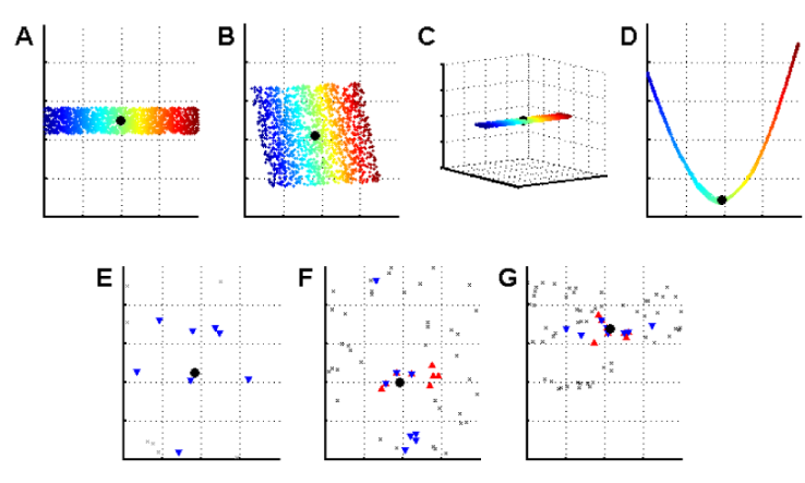
Figure 1: The output of LTSA (B) for the (two-dimensional) input shown in (A), where the input is a uniform sample from the strip $[0,1]\times[0,6]$. Ideally one would expect the two to be identical. The normalization constraint shortens the horizontal distances and lengthens the vertical distances, leading to the distortion of geodesic distances. (E) and (F) focus on the points shown in black in (A) and (B), respectively. The blue triangles in (E) and (F) are the $8$-nearest-neighborhood of the point denoted by the full black circle. The red triangles in (F) indicate the neighborhood computed for the corresponding point (full black circle) in the output space. Note that less than half of the original neighbors of the point remain neighbors in the output space. The input (A) with the addition of Gaussian noise normal to the manifold and of variance $10^{-4}$ is shown in (C). The output of LTSA for the noisy input is shown in (D). (G) shows a closeup of the neighborhood of the point indicated by the black circle in (D).

The example we consider is a uniform sample from a two-dimensional strip, shown in Fig. 1A. Note that in this example, $\mathcal{D}=d$; i.e., the input data is identical to the original data. Fig. 1B presents the output of LTSA on the input in Fig. 1A. The most obvious difference between input and output is that while the input is a strip, the output is roughly square. While this may seem to be of no importance, note that it means that the algorithm, like all the normalized-output algorithms, does not preserve geodesic distances even up to a scaling factor. By definition, the geodesic distance between two points on a manifold is the length of the shortest path on the manifold between the two points. Preservation of geodesic distances is particularly relevant when the manifold is isometrically embedded. In this case, assuming the domain is convex, the geodesic distance between any two points on the manifold is equal to the Euclidean distance between the corresponding domain points. Geodesic distances are conserved, for example, by the Isomap algorithm (Tenenbaum et al., 2000).

Figs. 1E and 1F present closeups of Figs. 1A and 1B, respectively. Here, a less obvious phenomenon is revealed: the structure of the local neighborhood is not preserved by LTSA. By local structure we refer to the angles and distances (at least up to a scale) between all points within each local neighborhood. Mappings that preserve local structures up to a scale are called conformal mappings (see for example de Silva and Tenenbaum, 2003; Sha and Saul, 2005). In addition to the distortion of angles and distances, the $K$-nearest-neighbors of a given point on the manifold do not necessarily correspond to the $K$-nearest-neighbors of the respective output point, as shown in Figs. 1E and 1F. Accordingly, we conclude that the original structure of the local neighborhoods is not necessarily preserved by the normalized-output algorithms.

The above discussion highlights the fact that one cannot expect the normalized-output algorithms to preserve geodesic distances or local neighborhood structure. However, it seems reasonable to demand that the output of the normalized-output algorithms resemble an affine transformation of the original sample. In fact, the output presented in Fig. 1B is an affine transformation of the input, which is the original sample, presented in Fig. 1A. A formal similarity criterion based on affine transformations is given by Huo and Smith (2006). In the following, we will claim that a normalized-output algorithm succeeds (or fails) based on the existence (or lack thereof) of resemblance between the output and the original sample, up to an affine transformation.

Fig. 1D presents the output of LTSA on a noisy version of the input, shown in Fig. 1C. In this case, the algorithm prefers an output that is roughly a one-dimensional curve embedded in $\mathbb{R}^{2}$. While this result may seem incidental, the results of all the other normalized-output algorithms for this example are essentially the same.

Using the affine transformation criterion, we can state that LTSA succeeds in recovering the underlying structure of the strip shown in Fig. 1A. However, in the case of the noisy strip shown in Fig. 1C, LTSA fails to recover the structure of the input. We note that all the other normalized-output algorithms perform similarly.

For practical purposes, we will now generalize the definition of failure of the normalized-output algorithms. This definition is more useful when it is necessary to decide whether an algorithm has failed, without actually computing the output. This is useful, for example, when considering the outputs of an algorithm for a class of manifolds.

We now present the generalized definition of failure of the algorithms. Let $X=X_{N\times d}$ be the original sample. Assume that the input is given by $\psi(X)\subset\mathbb{R}^{\mathcal{D}}$, where $\psi:\mathbb{R}^{d}\rightarrow\mathbb{R}^{\mathcal{D}}$ is some smooth function, and $\mathcal{D}\geq d$ is the dimension of the input. Let $Y=Y_{N\times d}$ be an affine transformation of the original sample $X$, such that the normalization constraints of Eq. 5 hold. Note that $Y$ is algorithm-dependent, and that for each algorithm, $Y$ is unique up to rotation and translation. When the algorithm succeeds it is expected that the output will be similar to a normalized version of $X$, namely to $Y$. Let $Z=Z_{N\times d}$ be any matrix that satisfies the same normalization constraints. We say that the algorithm has failed if $\Phi(Y)>\Phi(Z)$, and $Z$ is substantially different from $Y$, and hence also from $X$. In other words, we say that the algorithm has failed when a substantially different embedding $Z$ has a lower cost than the most appropriate embedding $Y$. A precise definition of “substantially different” is not necessary for the purposes of this paper. It is enough to consider $Z$ substantially different from $Y$ when $Z$ is of lower dimension than $Y$, as in Fig. 1D.

We emphasize that the matrix $Z$ is not necessarily similar to the output of the algorithm in question. It is a mathematical construction that shows when the output of the algorithm is not likely to be similar to $Y$, the normalized version of the true manifold structure. The following lemma shows that if $\Phi(Y)>\Phi(Z)$, the inequality is also true for a small perturbation of $Y$. Hence, it is not likely that an output that resembles $Y$ will occur when $\Phi(Y)>\Phi(Z)$ and $Z$ is substantially different from $Y$.

Lemma 3.1

Let $Y$ be an $N\times d$ matrix. Let $\widetilde{Y}=Y+\varepsilon E$ be a perturbation of $Y$, where $E$ is an $N\times d$ matrix such that $\left\|E\right\|_{F}=1$ and where $\varepsilon>0$. Let $S$ be the maximum number of neighborhoods to which a single input point belongs. Then for LLE with positive weights $w_{i,j}$, LEM, DFM, LTSA, and HLLE, we have

$$\Phi(\widetilde{Y})>(1-4\varepsilon)\Phi(Y)-4\varepsilon C_{a}S\,,$$

where $C_{a}$ is a constant that depends on the algorithm.

The use of positive weights in LLE is discussed in Saul and Roweis (2003, Section 5); a similar result for LLE with general weights can be obtained if one allows a bound on the values of $w_{i,j}$. The proof of Lemma 3.1 is given in Appendix A.2.

4 Analysis of the two-dimensional grid

In this section we analyze the performance of LEM on the two-dimensional grid. In particular, we argue that LEM cannot recover the structure of a two-dimensional grid in the case where the aspect ratio of the grid is greater than $2$. Instead, LEM prefers a one-dimensional curve in $\mathbb{R}^{2}$. Implications also follow for DFM, as explained in Section 4.3, followed by a discussion of the other normalized-output algorithms. Finally, we present empirical results that demonstrate our claims.

In Section 5 we prove a more general statement regarding any two-dimensional manifold. Necessary conditions for successful performance of the normalized-output algorithms on such manifolds are presented. However, the analysis in this section is important in itself for two reasons. First, the conditions for the success of LEM on the two-dimensional grid are more limiting. Second, the analysis is simpler and points out the reasons for the failure of all the normalized-output algorithms when the necessary conditions do not hold.

4.1 Possible embeddings of a two-dimensional grid

We consider the input data set $X$ to be the two-dimensional grid $[-m,\ldots,m]\times[-q,\ldots,q]$, where $m\geq q$. We denote $x_{ij}=(i,j)$. For convenience, we regard $X=(X^{(1)},X^{(2)})$ as an $N\times 2$ matrix, where $N=(2m+1)(2q+1)$ is the number of points in the grid. Note that in this specific case, the original sample and the input are the same.

In the following we present two different embeddings, $Y$ and $Z$. Embedding $Y$ is the grid itself, normalized so that $\mathrm{Cov}(Y)=I$. Embedding $Z$ collapses each column to a point and positions the resulting points in the two-dimensional plane in a way that satisfies the constraint $\mathrm{Cov}(Z)=I$ (see Fig. 2 for both). The embedding $Z$ is a curve in $\mathbb{R}^{2}$ and clearly does not preserve the original structure of the grid.

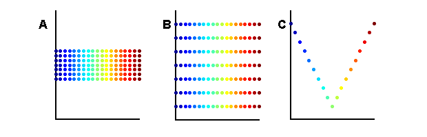
Figure 2: (A) The input grid. (B) Embedding $Y$, the normalized grid. (C) Embedding $Z$, a curve that satisfies $\mathrm{Cov}(Z)=I$.

We first define the embeddings more formally. We start by defining $\widehat{Y}=X(X^{\prime}DX)^{-1/2}$. Note that this is the only linear transformation of $X$ (up to rotation) that satisfies the conditions $\widehat{Y}^{\prime}D\textbf{1}=\textbf{0}$ and $\widehat{Y}^{\prime}D\widehat{Y}=I$, which are the normalization constraints for LEM (see Eq. 5). However, the embedding $\widehat{Y}$ depends on the matrix $D$, which in turn depends on the choice of neighborhoods. Recall that the matrix $D$ is a diagonal matrix, where $d_{ii}$ equals the number of neighbors of the $i$-th point. Choose $r$ to be the radius of the neighborhoods. Then, for all inner points $x_{ij}$, the number of neighbors $K(i,j)$ is a constant, which we denote as $K$. We shall call all points with less than $K$ neighbors boundary points. Note that the definition of boundary points depends on the choice of $r$. For inner points of the grid we have $d_{ii}\equiv K$. Thus, when $K\ll N$ we have $X^{\prime}DX\approx KX^{\prime}X$.

We define $Y=X\textrm{Cov}(X)^{-1/2}$. Note that $Y^{\prime}\textbf{1}=0$, $\textrm{Cov}(Y)=I$ and for $K\ll N$, $Y\approx\sqrt{KN}\widehat{Y}$. In this section we analyze the embedding $Y$ instead of $\widehat{Y}$, thereby avoiding the dependence on the matrix $D$ and hence simplifying the notation. This simplification does not significantly change the problem and does not affect the results we present. Similar results are obtained in the next section for general two-dimensional manifolds, using the exact normalization constraints (see Section 5.2).

Note that $Y$ can be described as the set of points $[-m/\sigma,\ldots,m/\sigma]\times[-q/\tau,\ldots,q/\tau]$, where $y_{ij}=(i/\sigma,j/\tau)$. The constants $\sigma^{2}=\textrm{Var}(X^{(1)})$ and $\tau^{2}=\textrm{Var}(X^{(2)})$ ensure that the normalization constraint $\mathrm{Cov}(Y)=I$ holds. Straightforward computation (see Appendix A.3) shows that

$$\sigma^{2}=\frac{(m+1)m}{3}\,;\;\tau^{2}=\frac{(q+1)q}{3}\,.$$ (6)

The definition of the embedding $Z$ is as follows:

$$z_{ij}=\left\{\begin{array}[]{cc}\left(\frac{i}{\sigma},\frac{-2i}{\rho}-\bar{z}^{(2)}\right)&i\leq 0\\ \\ \left(\frac{i}{\sigma},\frac{2i}{\rho}-\bar{z}^{(2)}\right)&i\geq 0\end{array}\right.\,,$$ (7)

where $\bar{z}^{(2)}=\frac{(2q+1)2}{N\rho}\sum_{i=1}^{m}(2i)$ ensures that $Z^{\prime}\textbf{1}=\textbf{0}$, and $\sigma$ (the same $\sigma$ as before; see below) and $\rho$ are chosen so that sample variance of $Z^{(1)}$ and $Z^{(2)}$ is equal to one. The symmetry of $Z^{(1)}$ about the origin implies that $\textrm{Cov}(Z^{(1)},Z^{(2)})=0$, hence the normalization constraint $\textrm{Cov}(Z)=I$ holds. $\sigma$ is as defined in Eq. 6, since $Z^{(1)}=Y^{(1)}$ (with both defined similarly to $X^{(1)}$). Finally, note that the definition of $z_{ij}$ does not depend on $j$.

4.2 Main result for LEM on the two-dimensional grid

We estimate $\Phi(Y)$ by $N\phi(Y_{ij})$ (see Eq. 4), where $y_{ij}$ is an inner point of the grid and $Y_{ij}$ is the neighborhood of $y_{ij}$; likewise, we estimate $\Phi(Z)$ by $N\phi(Z_{ij})$ for an inner point $z_{ij}$. For all inner points, the value of $\phi(Y_{ij})$ is equal to some value $\phi$. For boundary points, $\phi(Y_{ij})$ is bounded by $\phi$ multiplied by some constant that depends only on the number of neighbors. Hence, for large $m$ and $q$, the difference between $\Phi(Y)$ and $N\phi(Y_{ij})$ is negligible.

The main result of this section states:

Theorem 4.1

Let $y_{ij}$ be an inner point and let the ratio $\frac{m}{q}$ be greater than $2$. Then

$$\phi(Y_{ij})>\phi(Z_{ij})$$

for neighborhood-radius $r$ that satisfies $1\leq r\leq 3$, or similarly, for $K$-nearest neighborhoods where $K=4,8,12$.

This indicates that for aspect ratios $\frac{m}{q}$ that are greater than $2$ and above, mapping $Z$, which is essentially one-dimensional, is preferred to $Y$, which is a linear transformation of the grid. The case of general $r$-ball neighborhoods is discussed in Appendix A.4 and indicates that similar results should be expected.

The proof of the theorem is as follows. It can be shown analytically (see Fig. 3) that

$$\phi(Y_{ij})=F(K)\left(\frac{1}{\sigma^{2}}+\frac{1}{\tau^{2}}\right)\,,$$ (8)

where

$$F(4)=2\,;\;\;F(8)=6\,;\;\;F(12)=14\,.$$ (9)

For higher $K$, $F(K)$ can be approximated for any $r$-ball neighborhood of $y_{ij}$ (see Appendix A.4).

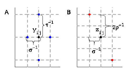
Figure 3: (A) The normalized grid at an inner point $y_{ij}$. The $4$-nearest-neighbors of $y_{ij}$ are marked in blue. Note that the neighbors from the left and from the right are at a distance of $1/\sigma$, while the neighbors from above and below are at a distance of $1/\tau$. The value of $\phi(Y_{ij})$ is equal to the sum of squared distances of $y_{ij}$ to its neighbors. Hence, we obtain that $\phi(Y_{ij})=2/\sigma^{2}+2/\tau^{2}$ when $K=4$ and $\phi(Y_{ij})=2/\sigma^{2}+2/\tau^{2}+4(1/\sigma^{2}+1/\tau^{2})$ when $K=8$. (B) The curve embedding at an inner point $z_{ij}$. The neighbors of $z_{ij}$ from the left and from the right are marked in red. The neighbors from above and below are embedded to the same point as $z_{ij}$. Note that the squared distance between $z_{ij}$ and $z_{(i\pm 1)j}$ equals $1/\sigma^{2}+4/\rho^{2}$. Hence, $\phi(Z_{ij})=2(1/\sigma^{2}+4/\rho^{2})$ when $K=4$, and $\phi(Z_{ij})=6(1/\sigma^{2}+4/\rho^{2})$ when $K=8$.

It can be shown (see Fig. 3) that

$$\phi(Z_{ij})=\widetilde{F}(K)\left(\frac{1}{\sigma^{2}}+\frac{4}{\rho^{2}}\right)\,,$$ (10)

where $\widetilde{F}(K)=F(K)$ for $K=4,8,12$. For higher $K$, it can be shown (see Appendix A.4) that $\widetilde{F}(K)\approx F(K)$ for any $r$-ball neighborhood.

A careful computation (see Appendix A.5) shows that

$$\rho>\sigma\,,$$ (11)

and therefore

$$\phi(Z_{ij})<\frac{5F(K)}{\sigma^{2}}\,.$$ (12)

Assume that $\frac{m}{q}>2$. Since both $m$ and $q$ are integers, we have that $m+1\geq 2(q+1)$. Hence, using Eq. 6 we have

$$\sigma^{2}=\frac{m(m+1)}{3}>\frac{4q(q+1)}{3}=4\tau^{2}\,.$$

Combining this result with Eqs. 8 and 12 we have

$$\frac{m}{q}>2\Rightarrow\phi(Y_{ij})>\phi(Z_{ij})\,.$$

which proves Theorem 4.1.

4.3 Implications to other algorithms

We start with implications regarding DFM. There are two main differences between LEM and DFM. The first difference is the choice of the kernel. LEM chooses $w_{i,j}=1$, which can be referred to as the “window” kernel (a Gaussian weight function was also considered by Belkin and Niyogi, 2003). DFM allows a more general rotation-invariant kernel, which includes the “window” kernel of LEM. The second difference is that DFM renormalizes the weights $k_{\varepsilon}(x_{i},x_{i,j})$ (see Eq. 2). However, for all the inner points of the grid with neighbors that are also inner points, the renormalization factor $(q_{\varepsilon}(x_{i})^{-1}q_{\varepsilon}(x_{i,j})^{-1})$ is a constant. Therefore, if DFM chooses the “window” kernel, it is expected to fail, like LEM. In other words, when DFM using the “window” kernel is applied to a grid with aspect ratio slightly greater than $2$ or above, DFM will prefer the embedding $Z$ over the embedding $Y$ (see Fig 2). For a more general choice of kernel, the discussion in Appendix A.4 indicates that a similar failure should occur. This is because the relation between the estimations of $\Phi(Y)$ and $\Phi(Z)$ presented in Eqs. 8 and 10 holds for any rotation-invariant kernel (see Appendix A.4). This observation is also evident in numerical examples, as shown in Figs. 4 and 5.

In the cases of LLE with no regularization, LTSA, and HLLE, it can be shown that $\Phi(Y)\equiv 0$. Indeed, for LTSA and HLLE, the weight matrix $W_{i}$ projects on a space that is perpendicular to the SVD of the neighborhood $X_{i}$, thus $\left\|W_{i}X_{i}\right\|_{F}^{2}=0$. Since $Y_{i}=X_{i}\textrm{Cov}(X)^{-1/2}$, we have $\left\|W_{i}Y_{i}\right\|_{F}^{2}=0$, and, therefore, $\Phi(Y)\equiv 0$. For the case of LLE with no regularization, when $K\geq 3$, each point can be reconstructed perfectly from its neighbors, and the result follows. Hence, a linear transformation of the original data should be the preferred output. However, the fact that $\Phi(Y)\equiv 0$ relies heavily on the assumption that both the input $X$ and the output $Y$ are of the same dimension (see Theorem 5.1 for manifolds embedded in higher dimensions), which is typically not the case in dimension-reducing applications.

4.4 Numerical results

For the following numerical results, we used the Matlab implementation written by the respective algorithms’ authors as provided by Wittman (retrieved Jan. 2007) (a minor correction was applied to the code of HLLE).

We ran the LEM algorithm on data sets with aspect ratios above and below $2$. We present results for both a grid and a uniformly sampled strip. The neighborhoods were chosen using $K$-nearest neighbors with $K=4,8,16$, and $64$. We present the results for $K=8$; the results for $K=4,16$, and $64$ are similar. The results for the grid and the random sample are presented in Figs. 4 and 5, respectively.

We ran the DFM algorithm on the same data sets. We used the normalization constant $\alpha=1$ and the kernel width $\sigma=2$; the results for $\sigma=1,4$, and $8$ are similar. The results for the grid and the random sample are presented in Figures 4 and 5, respectively.

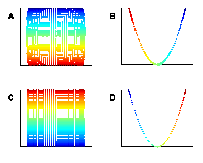
Figure 4: The output of LEM on a grid of dimensions $81\times 41$ is presented in (A). The result of LEM for the grid of dimensions $81\times 39$ is presented in (B). The number of neighbors in both computations is $8$. The output for DFM on the same data sets using $\sigma=2$ appears in (C) and (D), respectively.

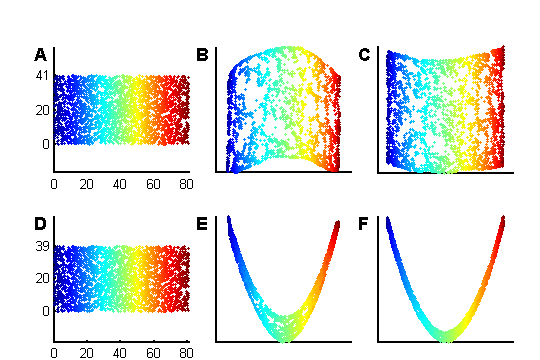
Figure 5: (A) and (D) show the same 3000 points, uniformly-sampled from the unit square, scaled to the areas $[0,81]\times[0,41]$ and $[0,81]\times[0,39]$, respectively. (B) and (E) show the outputs of LEM for inputs (A) and (D), respectively. The number of neighbors is both computations is $8$. (C) and (F) show the output for DFM on the same data sets using $\sigma=2$. Note the sharp change in output structure for extremely similar inputs.

Both examples clearly demonstrate that for aspect ratios sufficiently greater than $2$, both LEM and DFM prefer a solution that collapses the input data to a nearly one-dimensional output, normalized in $\mathbb{R}^{2}$. This is exactly as expected, based on our theoretical arguments.

Finally, we ran LLE, HLLE, and LTSA on the same data sets. In the case of the grid, both LLE and LTSA (roughly) recovered the grid shape for $K=4,8,16$, and $64$, while HLLE failed to produce any output due to large memory requirements. In the case of the random sample, both LLE and HLLE succeeded for $K=16,64$ but failed for $K=4,8$. LTSA succeeded for $K=8,16$, and $64$ but failed for $K=4$. The reasons for the failure for lower values of $K$ are not clear, but may be due to roundoff errors. In the case of LLE, the failure may also be related to the use of regularization in LLE’s second step.

5 Analysis for general two-dimensional manifolds

The aim of this section is to present necessary conditions for the success of the normalized-output algorithms on general two-dimensional manifolds embedded in high-dimensional space. We show how this result can be further generalized to manifolds of higher dimension. We demonstrate the theoretical results using numerical examples.

5.1 Two different embeddings for a two-dimensional manifold

We start with some definitions. Let $X=[x_{1},\ldots,x_{N}]^{\prime},\,x_{i}\in\mathbb{R}^{2}$ be the original sample. Without loss of generality, we assume that

$$\bar{x}=\mathbf{0};\;\;\;\;\;\mathrm{Cov}(X)\equiv\Sigma=\left(\begin{array}[]{cc}\sigma^{2}&0\\ 0&\tau^{2}\\ \end{array}\right)\,.$$

As in Section 4, we assume that $\sigma>\tau$. Assume that the input for the normalized-output algorithms is given by $\psi(X)\subset\mathbb{R}^{\mathcal{D}}$ where $\psi:\mathbb{R}^{2}\rightarrow\mathbb{R}^{\mathcal{D}}$ is a smooth function and $\mathcal{D}\geq 2$ is the dimension of the input. When the mapping $\psi$ is an isometry, we expect $\Phi(X)$ to be small. We now take a close look at $\Phi(X)$.

$$\Phi(X)=\sum_{i=1}^{N}\left\|W_{i}X_{i}\right\|^{2}_{F}=\sum_{i=1}^{N}\left\|W_{i}X_{i}^{(1)}\right\|^{2}+\sum_{i=1}^{N}\left\|W_{i}X_{i}^{(2)}\right\|^{2}\,,$$

where $X_{i}^{(j)}$ is the $j$-th column of the neighborhood $X_{i}$. Define $e_{i}^{(j)}=\left\|W_{i}X_{i}^{(j)}\right\|^{2}$, and note that $e_{i}^{(j)}$ depends on the different algorithms through the definition of the matrices $W_{i}$. The quantity $e_{i}^{(j)}$ is the portion of error obtained by using the $j$-th column of the $i$-th neighborhood when using the original sample as output. Denote $\bar{e}^{(j)}=\frac{1}{N}\sum_{i}e_{i}^{(j)}$, the average error originating from the $j$-th column.

We define two different embeddings for $\psi(X)$, following the logic of Sec. 4.1. Let

$$Y=X\Sigma^{-1/2}$$ (13)

be the first embedding. Note that $Y$ is just the original sample up to a linear transformation that ensures that the normalization constraints $\textrm{Cov}(Y)=I$ and $Y^{\prime}\textbf{1}=\textbf{0}$ hold. Moreover, $Y$ is the only transformation of $X$ that satisfies these conditions, which are the normalization constraints for LLE, HLLE, and LTSA. In Section 5.2 we discuss the modified embeddings for LEM and DFM.

The second embedding, $Z$, is given by

$$z_{i}=\left\{\begin{array}[]{cc}\left(\frac{x_{i}^{(1)}}{\sigma},\frac{-x_{i}^{(1)}}{\rho}-\bar{z}^{(2)}\right)&x_{i}^{(1)}<0\\ \\ \left(\frac{x_{i}^{(1)}}{\sigma},\frac{\kappa x_{i}^{(1)}}{\rho}-\bar{z}^{(2)}\right)&x_{i}^{(1)}\geq 0\end{array}\right.\,.$$ (14)

Here

$$\kappa=\Big{(}\sum_{i:x_{i}^{(1)}<0}\Big{(}x_{i}^{(1)}\Big{)}^{2}\Big{)}^{1/2}\Big{(}\sum_{i:x_{i}^{(1)}\geq 0}\Big{(}x_{i}^{(1)}\Big{)}^{2}\Big{)}^{-1/2}\,$$ (15)

ensures that $\mathrm{Cov}(Z^{(1)},Z^{(2)})=0$, and $\bar{z}^{(2)}=\frac{1}{N}(\sum_{x_{i}^{(1)}\geq 0}\frac{\kappa x_{i}^{(1)}}{\rho}+\sum_{x_{i}^{(1)}<0}\frac{-x_{i}^{(1)}}{\rho})$ and $\rho$ are chosen so that the sample mean and variance of $Z^{(2)}$ are equal to zero and one, respectively. We assume without loss of generality that $\kappa\geq 1$.

Note that $Z$ depends only on the first column of $X$. Moreover, each point $z_{i}$ is just a linear transformation of $x_{i}^{(1)}$. In the case of neighborhoods $Z_{i}$, the situation can be different. If the first column of $X_{i}$ is either non-negative or non-positive, then $Z_{i}$ is indeed a linear transformation of $X_{i}^{(1)}$. However, if $X_{i}^{(1)}$ is located on both sides of zero, $Z_{i}$ is not a linear transformation of $X_{i}^{(1)}$. Denote by $N_{0}$ the set of indices $i$ of neighborhoods $Z_{i}$ that are not linear transformations of $X_{i}^{(1)}$. The number $|N_{0}|$ depends on the number of nearest neighbors $K$. Recall that for each neighborhood, we defined the radius $r(i)=\max_{j,k\in\{0,\ldots,K\}}\left\|x_{i,j}-x_{i,k}\right\|$. Define $r_{\max}=\max_{i\in N_{0}}r(i)$ to be the maximum radius of neighborhoods $i$, such that $i\in N_{0}$.

5.2 The embeddings for LEM and DFM

So far we have claimed that given the original sample $X$, we expect the output to resemble $Y$ (see Eq. 13). However, $Y$ does not satisfy the normalization constraints of Eq. 5 for the cases of LEM and DFM. Define $\hat{Y}$ to be the only affine transformation of $X$ (up to rotation) that satisfies the normalization constraint of LEM and DFM. When the original sample is given by $X$, we expect the output of LEM and DFM to resemble $\hat{Y}$. We note that unlike the matrix $Y$ that was defined in terms of the matrix $X$ only, $\hat{Y}$ depends also on the choice of neighborhoods through the matrix $D$ that appears in the normalization constraints.

We define $\hat{Y}$ more formally. Denote $\widetilde{X}=X-\frac{1}{\textbf{1}^{\prime}D\textbf{1}}\textbf{1}\textbf{1}^{\prime}DX$. Note that $\widetilde{X}$ is just a translation of $X$ that ensures that $\widetilde{X}^{\prime}D\textbf{1}=\textbf{0}$. The matrix $\widetilde{X}^{\prime}D\widetilde{X}$ is positive definite and therefore can be presented by $\Gamma\widehat{\Sigma}\Gamma^{\prime}$ where $\Gamma$ is a $2\times 2$ orthogonal matrix and

$$\widehat{\Sigma}=\left(\begin{array}[]{cc}\hat{\sigma}^{2}&0\\ 0&\hat{\tau}^{2}\\ \end{array}\right)\,,$$

where $\hat{\sigma}\geq\hat{\tau}$. Define $\widehat{X}=\widetilde{X}\Gamma$; then $\widehat{Y}=\widehat{X}\widehat{\Sigma}^{-1/2}$ is the only affine transformation of $X$ that satisfies the normalization constraints of LEM and DFM; namely, we have $\widehat{Y}^{\prime}D\widehat{Y}=I$ and $\widehat{Y}^{\prime}D\textbf{1}=\textbf{0}$.

We define $\widehat{Z}$ similarly to Eq. 14,

$$\hat{z}_{i}=\left\{\begin{array}[]{cc}\left(\frac{\hat{x}_{i}^{(1)}}{\hat{\sigma}},\frac{-\hat{x}_{i}^{(1)}}{\hat{\rho}}-\hat{\bar{z}}^{(2)}\right)&\hat{x}_{i}^{(1)}<0\\ \\ \left(\frac{\hat{x}_{i}^{(1)}}{\hat{\sigma}},\frac{\hat{\kappa}\hat{x}_{i}^{(1)}}{\hat{\rho}}-\hat{\bar{z}}^{(2)}\right)&\hat{x}_{i}^{(1)}\geq 0\end{array}\right.\,,$$

where $\hat{\kappa}$ is defined by Eq. 15 with respect to $\widehat{X}$, $\hat{\bar{z}}^{(2)}=\frac{1}{N}(\sum_{x_{i}^{(1)}\geq 0}\frac{d_{ii}\hat{\kappa}x_{i}^{(1)}}{\rho}+\sum_{x_{i}^{(1)}<0}\frac{-d_{ii}x_{i}^{(1)}}{\rho})$ and $\hat{\rho}^{2}=\kappa^{2}\sum_{\hat{x}_{i}^{(1)}\geq 0}d_{ii}\left(\hat{x}_{i}^{(1)}\right)^{2}+\sum_{\hat{x}_{i}^{(1)}\leq 0}d_{ii}\left(\hat{x}_{i}^{(1)}\right)^{2}$.

A similar analysis to that of $Y$ and $Z$ can be performed for $\widehat{Y}$ and $\widehat{Z}$. The same necessary conditions for success are obtained, with $\sigma$, $\tau$, and $\rho$ replaced by $\hat{\sigma}$, $\hat{\tau}$, and $\hat{\rho}$, respectively. In the case where the distribution of the original points is uniform, the ratio $\frac{\hat{\sigma}}{\hat{\tau}}$ is close to the ratio $\frac{\sigma}{\tau}$ and thus the necessary conditions for the success of LEM and DFM are similar to the conditions in Corollary 5.2.

5.3 Characterization of the embeddings

The main result of this section provides necessary conditions for the success of the normalized-output algorithms. Following Section 3, we say that the algorithms fail if $\Phi(Y)>\Phi(Z)$, where $Y$ and $Z$ are defined in Eqs. 13 and 14, respectively. Thus, a necessary condition for the success of the normalized-output algorithms is that $\Phi(Y)\leq\Phi(Z)$.

Theorem 5.1

Let $X$ be a sample from a two-dimensional domain and let $\psi(X)$ be its embedding in high-dimensional space. Let $Y$ and $Z$ be defined as above. Then

$$\frac{\kappa^{2}}{\rho^{2}}\left(\bar{e}^{(1)}+\frac{|N_{0}|}{N}c_{a}r_{\max}^{2}\right)<\frac{\bar{e}^{(2)}}{\tau^{2}}\quad\Longrightarrow\quad\Phi(Y)>\Phi(Z)\,,$$

where $c_{a}$ is a constant that depends on the specific algorithm. For the algorithms LEM and DFM a more restrictive condition can be defined:

$$\frac{\kappa^{2}}{\rho^{2}}\bar{e}^{(1)}<\frac{\bar{e}^{(2)}}{\tau^{2}}\quad\Longrightarrow\quad\Phi(Y)>\Phi(Z)\,.$$

For the proof, see Appendix A.6.

Adding some assumptions, we can obtain a simpler criterion. First note that, in general, $\bar{e}^{(1)}$ and $\bar{e}^{(2)}$ should be of the same order, since it can be assumed that, locally, the neighborhoods are uniformly distributed. Second, following Lemma A.2 (see Appendix A.8), when $X^{(1)}$ is a sample from a symmetric unimodal distribution it can be assumed that $\kappa\approx 1$ and $\rho^{2}>\frac{\sigma^{2}}{8}$. Then we have the following corollary:

Corollary 5.2

Let $X,Y,Z$ be as in Theorem 5.1. Let $c=\sigma/\tau$ be the ratio between the variance of the first and second columns of $X$. Assume that $\bar{e}^{(1)}<\sqrt{2}\bar{e}^{(2)}$, $\kappa<\sqrt[4]{2}$, and $\rho^{2}>\frac{\sigma^{2}}{8}$. Then

$$4\left(1+\frac{|N_{0}|}{N}\frac{c_{a}r_{\max}^{2}}{\sqrt{2}\bar{e}^{(2)}}\right)<c\Rightarrow\Phi(Y)>\Phi(Z)\,.$$

For LEM and DFM, we can write

$$4<c\Rightarrow\Phi(Y)>\Phi(Z)\,.$$

We emphasize that both Theorem 5.1 and Corollary 5.2 do not state that $Z$ is the output of the normalized-output algorithms. However, when the difference between the right side and the left side of the inequalities is large, one cannot expect the output to resemble the original sample (see Lemma 3.1). In these cases we say that the algorithms fail to recover the structure of the original domain.

5.4 Generalization of the results to manifolds of higher dimensions

The discussion above introduced necessary conditions for the normalized-output algorithms’ success on two-dimensional manifolds embedded in $\mathbb{R}^{\mathcal{D}}$. Necessary conditions for success on general $d$-dimensional manifolds, $d\geq 3$, can also be obtained. We present here a simple criterion to demonstrate the fact that there are $d$-dimensional manifolds that the normalized-output algorithms cannot recover.

Let $X=[X^{(1)},\ldots,X^{(d)}]$ be a $N\times d$ sample from a $d$-dimensional domain. Assume that the input for the normalized-output algorithms is given by $\psi(X)\subset\mathbb{R}^{\mathcal{D}}$ where $\psi:\mathbb{R}^{d}\rightarrow\mathbb{R}^{\mathcal{D}}$ is a smooth function and $\mathcal{D}\geq d$ is the dimension of the input. We assume without loss of generality that $X^{\prime}\textbf{1}=\textbf{0}$ and that $\textrm{Cov}(X)$ is a diagonal matrix. Let $Y=X\textrm{Cov}(X)^{-1/2}$. We define the matrix $Z=[Z^{(1)},\ldots,Z^{(d)}]$ as follows. The first column of $Z$, $Z^{(1)}$, equals the first column of $Y$, namely, $Z^{(1)}=Y^{(1)}$. We define the second column $Z^{(2)}$ similarly to the definition in Eq. 14:

$$Z^{(2)}_{i}=\left\{\begin{array}[]{cc}\frac{-x_{i}^{(1)}}{\rho}-\bar{z}^{(2)}&x_{i}^{(1)}<0\\ \\ \frac{\kappa x_{i}^{(1)}}{\rho}-\bar{z}^{(2)}&x_{i}^{(1)}\geq 0\end{array}\right.\,,$$

where $\kappa$ is defined as in Eq. 15, and $\bar{z}^{(2)}$ and $\rho$ are chosen so that the sample mean and variance of $Z^{(2)}$ are equal to zero and one, respectively. We define the next $d-2$ columns of $Z$ by

$$Z^{(j)}=\frac{Y^{(j)}-\sigma_{2j}Z^{(2)}}{\sqrt{1-\sigma_{2j}^{2}}}\,;\quad j=3,\ldots,d\,,$$

where $\sigma_{2j}=Z^{(2)}{}^{\prime}Y^{(j)}$. Note that $Z^{\prime}\textbf{1}=\textbf{0}$ and $\textrm{Cov}(Z)=I$. Denote $\sigma_{\max}=\max_{j\in\{3,\ldots,d\}}\sigma_{2j}$.

We bound $\Phi(Z)$ from above:

$$\Phi(Z) = \Phi(Y^{(1)})+\Phi(Z^{(2)})+\sum_{i=1}^{N}\left(\frac{1}{1-\sigma_{2j}^{2}}\right)\sum_{j=3}^{d}\left\|W_{i}\left(Y_{i}^{(j)}-\sigma_{2j}Z_{i}^{(2)}\right)\right\|^{2}$$

$$\leq \Phi(Y^{(1)})+\Phi(Z^{(2)})+\frac{1}{1-\sigma_{\max}^{2}}\sum_{i=1}^{N}\sum_{j=3}^{d}\left\|W_{i}Y_{i}^{(j)}\right\|^{2}+\frac{\sigma_{\max}^{2}}{1-\sigma_{\max}^{2}}\sum_{i=1}^{N}\sum_{j=3}^{d}\left\|W_{i}Z_{i}^{(2)}\right\|^{2}$$

$$= \Phi(Y^{(1)})+\frac{1+(d-3)\sigma_{\max}^{2}}{1-\sigma_{\max}^{2}}\Phi(Z^{(2)})+\frac{1}{1-\sigma_{\max}^{2}}\sum_{j=3}^{d}\Phi(Y^{(j)})\,.$$

Since we may write $\Phi(Y)=\sum_{j=1}^{d}\Phi(Y^{(j)})$, we have

$$\frac{1+(d-3)\sigma_{\max}^{2}}{1-\sigma_{\max}^{2}}\Phi(Z^{(2)})<\Phi(Y^{(2)})+\frac{\sigma_{\max}^{2}}{1-\sigma_{\max}^{2}}\sum_{j=3}^{d}\Phi(Y^{(j)})\Rightarrow\Phi(Z)<\Phi(Y)\,.$$

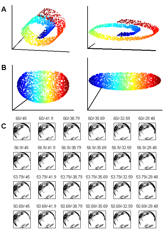
Figure 6: The data sets for the first example appear in panel A. In the left appears the $1600$-point original swissroll and in the right appears the same swissroll, after its first dimension was stretched by a factor of $3$. The data for the second example appear in panel B. In the left appears a $2400$-point uniform sample from the “fishbowl”, and in the right appears the same “fishbowl”, after its first dimension was stretched by a factor of $4$. In panel C appears the upper left corner of the array of $100\times 100$ pixel images of the globe. Above each image we write the elevation and azimuth.

When the sample is taken from a symmetric distribution with respect to the axes, one can expect $\sigma_{\max}$ to be small. In the specific case of the $d$-dimensional grid, $\sigma_{\max}=0$. Indeed, $Y^{(j)}$ is symmetric around zero, and all values of $Z^{(2)}$ appear for a given value of $Y^{(j)}$. Hence, both LEM and DFM are expected to fail whenever the ratio between the length of the grid in the first and second coordinates is slightly greater than $2$ or more, regardless of the length of grid in the other coordinates, similar to the result presented in Theorem 4.1. Corresponding results for the other normalized-output algorithms can also be obtained, similar to the derivation of Corollary 5.2.

5.5 Numerical results

We ran all five normalized-output algorithms, along with Isomap, on three data sets. We used the Matlab implementations written by the algorithms’ authors as provided by Wittman (retrieved Jan. 2007).

The first data set is a $1600$-point sample from the swissroll as obtained from Wittman (retrieved Jan. 2007). The results for the swissroll are given in Fig. 7, A1-F1. The results for the same swissroll, after its first dimension was stretched by a factor $3$, are given in Fig. 7, A2-F2. The original and stretched swissrolls are presented in Fig. 6A. The results for $K=8$ are given in Fig. 7. We also checked for $K=12,16$; but “short-circuits” occur (see Balasubramanian et al., 2002, for a definition and discussion of “short-circuits”).

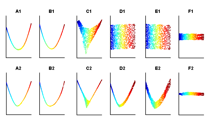
Figure 7: The output of LEM on $1600$ points sampled from a swissroll is presented in A1. The output of LEM on the same swissroll after stretching its first dimension by a factor of $3$ is presented in A2. Similarly, the outputs of DFM, LLE, LTSA, HLLE, and Isomap are presented in B1-2, C1-2, D1-2, E1-2, and F1-2, respectively. We used $K=8$ for all algorithms except DFM, where we used $\sigma=2$.

The second data set consists of $2400$ points, uniformly sampled from a “fishbowl”, where a “fishbowl” is a two-dimensional sphere minus a neighborhood of the northern pole (see Fig. 6B for both the “fishbowl” and its stretched version). The results for $K=8$ are given in Fig. 8. We also checked for $K=12,16$; the results are roughly similar. Note that the “fishbowl” is a two-dimensional manifold embedded in $\mathbb{R}^{3}$, which is not an isometry. While our theoretical results were proved under the assumption of isometry, this example shows that the normalized-output algorithms prefer to collapse their output even in more general settings.

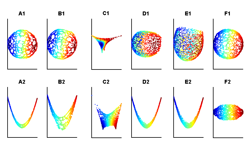
Figure 8: The output of LEM on $2400$ points sampled from a “fishbowl” is presented in A1. The output of LEM on the same “fishbowl” after stretching its first dimension by a factor of $4$ is presented in A2. Similarly, the outputs of DFM, LLE, LTSA, HLLE, and Isomap are presented in B1-2, C1-2, D1-2, E1-2, and F1-2, respectively. We used $K=8$ for all algorithms except DFM, where we used $\sigma=2$.

The third data set consists of $900$ images of the globe, each of $100\times 100$ pixels (see Fig. 6C). The images, provided by Hamm et al. (2005), were obtained by changing the globe’s azimuthal and elevation angles. The parameters of the variations are given by a $30\times 30$ array that contains $-45$ to $45$ degrees of azimuth and $-30$ to $60$ degrees of elevation. We checked the algorithms both on the entire set of images and on a strip of $30\times 10$ angular variations. The results for $K=8$ are given in Fig. 9. We also checked for $K=12,16$; the results are roughly similar.

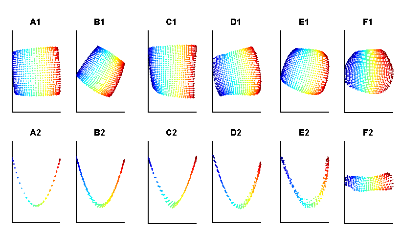
Figure 9: The output of LEM on the $30\times 30$ array of the globe rotation images is presented in A1; the output of LEM on the array of $30\times 10$ is presented in A2. Similarly, the outputs of DFM, LLE, LTSA, HLLE, and Isomap are presented in B1-2, C1-2, D1-2, E1-2, and F1-2 respectively. We used $K=8$ for all algorithms except DFM, where we chose $\sigma$ to be the root of the average distance between neighboring points.

These three examples, in addition to the noisy version of the two-dimensional strip discussed in Section 3 (see Fig. 1), clearly demonstrate that when the aspect ratio is sufficiently large, all the normalized-output algorithms prefer to collapse their output.

6 Asymptotics

In the previous sections we analyzed the phenomenon of global distortion obtained by the normalized-output algorithms on a finite input sample. However, it is of great importance to explore the limit behavior of the algorithms, i.e., the behavior when the number of input points tends to infinity. We consider the question of convergence in the case of input that consists of a $d$-dimensional manifold embedded in $\mathbb{R}^{\mathcal{D}}$, where the manifold is isometric to a convex subset of Euclidean space. By convergence we mean recovering the original subset of $\mathbb{R}^{d}$ up to a non-singular affine transformation.

Some previous theoretical works presented results related to the convergence issue. Huo and Smith (2006) proved convergence of LTSA under some conditions. However, to the best of our knowledge, no proof or contradiction of convergence has been given for any other of the normalized-output algorithms. In this section we discuss the various algorithms separately. We also discuss the influence of noise on the convergence. Using the results from previous sections, we show that there are classes of manifolds on which the normalized-output algorithms cannot be expected to recover the original sample, not even asymptotically.

6.1 LEM and DFM

Let $x_{1},x_{2},\ldots$ be a uniform sample from the two-dimensional strip $S=[0,L]\times[0,1]$. Let $X_{n}=[x_{1},\ldots,x_{n}]^{\prime}$ be the sample of size $n$. Let $K=K(n)$ be the number of nearest neighbors. Then when $K\ll n$ there exists with probability one an $N$, such that for all $n>N$ the assumptions of Corollary 5.2 hold. Thus, if $L>4$ we do not expect either LEM or DFM to recover the structure of the strip as the number of points in the sample tends to infinity. Note that this result does not depend on the number of neighbors or the width of the kernel, which can be changed as a function of the number of points $n$, as long as $K\ll n$. Hence, we conclude that LEM and DFM generally do not converge, regardless of the choice of parameters.

In the rest of this subsection we present further explanations regarding the failure of LEM and DFM based on the asymptotic behavior of the graph Laplacian (see Belkin and Niyogi, 2003, for details). Although it was not mentioned explicitly in this paper, it is well known that the outputs of LEM and DFM are highly related to the lower non-negative eigenvectors of the normalized graph Laplacian matrix (see Appendix A.1). It was shown by Belkin and Niyogi (2005), Hein et al. (2005), and Singer (2006) that the graph Laplacian operator converges to the continuous Laplacian operator. Thus, taking a close look at the eigenfunctions of the continuous Laplacian operator may reveal some additional insight into the behavior of both LEM and DFM.

Our working example is the two-dimensional strip $S=[0,L]\times[0,1]$, which can be considered as the continuous counterpart of the grid $X$ defined in Section 4. Following Coifman and Lafon (2006) we impose the Neumann boundary condition (see details therein). The eigenfunctions $\varphi_{i,j}(x_{1},x_{2})$ and eigenvalues $\lambda_{i,j}$ on the strip $S$ under these conditions are given by

$$\varphi_{i,j}(x_{1},x_{2})=\cos\left(\frac{i\pi}{L}x_{1}\right)\cos\left(j\pi x_{2}\right)\;\;\;\lambda_{i,j}=\left(\frac{i\pi}{L}\right)^{2}+\left(j\pi\right)^{2}\;\;\;\mathrm{for}\;i,j=0,1,2,\ldots\,.$$

When the aspect ratio of the strip satisfies $L>M\in\mathbb{N}$, the first $M$ non-trivial eigenfunctions are $\varphi_{i,0},\;i=1,\ldots,M$, which are functions only of the first variable $x_{1}$. Any embedding of the strip based on the first $M$ eigenfunctions is therefore a function of only the first variable $x_{1}$. Specifically, whenever $L>2$ the two-dimensional embedding is a function of the first variable only, and therefore clearly cannot establish a faithful embedding of the strip. Note that here we have obtained the same ratio constant $L>2$ computed for the grid (see Section 4 and Figs. 4 and 5) and not the looser constant $L>4$ that was obtained in Corollary 5.2 for general manifolds.

6.2 LLE, LTSA and HLLE

As mentioned in the beginning of this section, Huo and Smith (2006) proved the convergence of the LTSA algorithm. The authors of HLLE proved that the continuous manifold can be recovered by finding the null space of the continuous Hessian operator (see Donoho and Grimes, 2004, Corollary). However, this is not a proof that the algorithm HLLE converges. In the sequel, we try to understand the relation between Corollary 5.2 and the convergence proof of LTSA.

Let $x_{1},x_{2},\ldots$ be a sample from a compact and convex domain $\Omega$ in $\mathbb{R}^{2}$. Let $X_{n}=[x_{1},\ldots,x_{n}]^{\prime}$ be the sample of size $n$. Let $\psi$ be an isometric mapping from $\mathbb{R}^{2}$ to $\mathbb{R}^{\mathcal{D}}$, where $\mathcal{D}>2$. Let $\psi(X_{n})$ be the input for the algorithms. We assume that there is an $N$ such that for all $n>N$ the assumptions of Corollary 5.2 hold. This assumption is reasonable, for example, in the case of a uniform sample from the strip $S$. In this case Corollary 5.2 states that $\Phi(Z_{n})<\Phi(Y_{n})$ whenever

$$4\left(1+\frac{|n_{0}|}{n}\frac{c_{a}r_{\max,n}^{2}}{\sqrt{2}\bar{e}_{n}^{(2)}}\right)<c_{n}\,,$$

where $c_{n}$ is the ratio between the variance of $X_{n}^{(1)}$ and $X_{n}^{(2)}$ assumed to converge to a constant $c$. The expression $\frac{|n_{0}|}{n}$ is the fraction of neighborhoods $X_{i,n}$ such that $X_{i,n}^{(1)}$ is located on both sides of zero. $r_{\max,n}$ is the maximum radius of neighborhood in $n_{0}$. Note that we expect both $\frac{|n_{0}|}{n}$ and $r_{\max,n}$ to be bounded whenever the radius of the neighborhoods does not increase. Thus, Corollary 5.2 tells us that if $\{\bar{e}_{n}^{(2)}\}$ is bounded from below, we cannot expect convergence from LLE, LTSA or HLLE when $c$ is large enough.

The consequence of this discussion is that a necessary condition for the convergence of LLE, LTSA and HLLE is that $\{\bar{e}_{n}^{(2)}\}$ (and hence, from the assumptions of Corollary 5.2, also $\{\bar{e}_{n}^{(1)}\}$) converges to zero. If the two-dimensional manifold $\psi(\Omega)$ is not contained in a linear two-dimensional subspace of $\mathbb{R}^{\mathcal{D}}$, the mean error $\bar{e}_{n}^{(2)}$ is typically not zero due to curvature. However, if the radii of the neighborhoods tend to zero while the number of points in each neighborhood tends to infinity, we expect $\bar{e}_{n}^{(2)}\rightarrow 0$ for both LTSA and HLLE. This is because the neighborhood matrices $W_{i}$ are based on the linear approximation of the neighborhood as captured by the neighborhood SVD. When the radius of the neighborhood tends to zero, this approximation gets better and hence the error tends to zero. The same reasoning works for LLE, although the use of regularization in the second step of LLE may prevent $\bar{e}_{n}^{(2)}$ from converging to zero (see Section 2).

We conclude that a necessary condition for convergence is that the radii of the neighborhoods tend to zero. In the presence of noise, this requirement cannot be fulfilled. Assume that each input point is of the form $\psi(x_{i})+\varepsilon_{i}$ where $\varepsilon_{i}\in\mathbb{R}^{\mathcal{D}}$ is a random error that is independent of $\varepsilon_{j}$ for $j\neq i$. We may assume that $\varepsilon_{i}\sim N(0,\alpha^{2}I)$, where $\alpha$ is a small constant. If the radius of the neighborhood is smaller than $\alpha$, the neighborhood cannot be approximated reasonably by a two-dimensional projection. Hence, in the presence of noise of a constant magnitude, the radii of the neighborhoods cannot tend to zero. In that case, LLE, LTSA and HLLE might not converge, depending on the ratio $c$. This observation seems to be known also to Huo and Smith, who wrote:

“… we assume $\alpha=o(r)$; i.e., we have $\frac{\alpha}{r}\rightarrow 0$, as $r\rightarrow 0$.

It is reasonable to require that the error bound ($\alpha$) be smaller than the size of the neighborhood ($r$), which is reflected in the above condition. Notice that this condition is also somewhat nonstandard, since the magnitude of the errors is assumed to depend on $n$, but it seems to be necessary to ensure the consistency of LTSA.”

Summarizing, convergence may be expected when $n\rightarrow\infty$, if no noise is introduced. If noise is introduced and if $\sigma/\tau$ is large enough (depending on the level of noise $\alpha$), convergence cannot be expected (see Fig. 1).

7 Concluding remarks

In the introduction to this paper we posed the following question: Do the normalized-output algorithms succeed in revealing the underlying low-dimensional structure of manifolds embedded in high-dimensional spaces? More specifically, does the output of the normalized-output algorithms resemble the original sample up to affine transformation?

The answer, in general, is no. As we have seen, Theorem 5.1 and Corollary 5.2 show that there are simple low-dimensional manifolds, isometrically embedded in high-dimensional spaces, for which the normalized-output algorithms fail to find the appropriate output. Moreover, the discussion in Section 6 shows that when noise is introduced, even of small magnitude, this result holds asymptotically for all the normalized-output algorithms. We have demonstrated these results numerically for four different examples: the swissroll, the noisy strip, the (non-isometrically embedded) “fishbowl”, and a real-world data set of globe images. Thus, we conclude that the use of the normalized-output algorithms on arbitrary data can be problematic.

The main challenge raised by this paper is the need to develop manifold-learning algorithms that have low computational demands, are robust against noise, and have theoretical convergence guarantees. Existing algorithms are only partially successful: normalized-output algorithms are efficient, but are not guaranteed to converge, while Isomap is guaranteed to converge, but is computationally expensive. A possible way to achieve all of the goals simultaneously is to improve the existing normalized-output algorithms. While it is clear that, due to the normalization constraints, one cannot hope for geodesic distances preservation nor for neighborhoods structure preservation, success as measured by other criteria may be achieved. A suggestion of improvement for LEM appears in Gerber et al. (2007), yet this improvement is both computationally expensive and lacks a rigorous consistency proof. We hope that future research finds additional ways to improve the existing methods, given the improved understanding of the underlying problems detailed in this paper.

Acknowledgments

We are grateful to the anonymous reviewers of present and earlier versions of this manuscript for their helpful suggestions. We thank an anonymous referee for pointing out errors in the proof of Lemma 3.1. We thank J. Hamm for providing the database of globe images. This research was supported in part by Israeli Science Foundation grant and in part by NSF, grant DMS-0605236.

A Detailed proofs and discussions

A.1 The equivalence of the algorithms’ representations

For LEM, note that according to our representation, one needs to minimize

$$\Phi(Y)=\sum_{i=1}^{N}\left\|W_{i}Y_{i}\right\|^{2}_{F}=\sum_{i=1}^{N}\sum_{j=1}^{K}w_{i,j}\|y_{i}-y_{i,j}\|^{2}\,,$$

under the constraints $Y^{\prime}D\textbf{1}=\textbf{0}$ and $Y^{\prime}DY=I$. Define $\hat{w}_{rs}=w_{r,j}$ if $s$ is the $j$-th neighbor of $r$ and zero otherwise. Define $\hat{D}$ to be the diagonal matrix such that $d_{rr}=\sum_{s=1}^{N}\hat{w}_{rs}$; note that $\hat{D}=D$. Using these definitions, one needs to minimize $\Phi(Y)=\sum_{r,s}\hat{w}_{rs}\|y_{r}-y_{s}\|^{2}$ under the constraints $Y^{\prime}\hat{D}\textbf{1}=\textbf{0}$ and $Y^{\prime}\hat{D}Y=I$, which is the the authors’ representation of the algorithm.

For DFM, as for LEM, we define the weights $\hat{w}_{rs}$. Define the $N\times N$ matrix $\hat{W}=\left(\hat{w}_{rs}\right)$. Define the matrix $D^{-1}\hat{W}$; note that this matrix is a Markovian matrix and that $v^{(0)}\equiv\textbf{1}$ is its eigenvector corresponding to eigenvalue $1$, which is the largest eigenvalue of the matrix. Let $v^{(p)}$, $p=1,\ldots,d$ be the next $d$ eigenvectors, corresponding to the next $d$ largest eigenvalues $\lambda_{p}$, normalized such that $v^{(p)}{}^{\prime}Dv^{(p)}=1$. Note that the vectors $v^{(0)},\ldots,v^{(d)}$ are also the eigenvectors of $I-D^{-1}W$ corresponding to the $d+1$ lowest eigenvalues. Thus, the matrix $[v^{(1)},\ldots,v^{(d)}]$ (up to rotation) can be computed by minimizing $\textrm{tr}\left(Y^{\prime}(D-W)Y\right)$ under the constraints $Y^{\prime}DY=I$ and $Y^{\prime}D\textbf{1}=\textbf{0}$. Simple computation shows (see Belkin and Niyogi, 2003, Eq. 3.1) that $\textrm{tr}\left(Y^{\prime}(D-W)Y\right)=\frac{1}{2}\sum_{r,s}\hat{w}_{rs}\|y_{r}-y_{s}\|^{2}$. We already showed that $\Phi(Y)=\sum_{r,s}\hat{w}_{rs}\|y_{r}-y_{s}\|^{2}$. Hence, minimizing $\textrm{tr}\left(Y^{\prime}(D-W)Y\right)$ under the constraints $Y^{\prime}DY=I$ and $Y^{\prime}D\textbf{1}=\textbf{0}$ is equivalent to minimizing $\Phi(Y)$ under the same constraints. The embedding suggested by Coifman and Lafon (2006) (up to rotation) is the matrix $\left[\lambda_{1}\frac{v^{(1)}}{\left\|v^{(1)}\right\|},\ldots,\lambda_{d}\frac{v^{(d)}}{\left\|v^{(d)}\right\|}\right]$. Note that this embedding can be obtained from the output matrix $Y$ by a simple linear transformation.

For LLE, note that according to our representation, one needs to minimize

$$\Phi(Y)=\sum_{i=1}^{N}\left\|W_{i}Y_{i}\right\|^{2}_{F}=\sum_{i=1}^{N}\|y_{i}-\sum_{j=1}^{K}w_{i,j}y_{i,j}\|^{2}$$

under the constraints $Y^{\prime}\textbf{1}=\textbf{0}$ and $\textrm{Cov}(Y)=I$, which is the minimization problem given by Roweis and Saul (2000).

The representation of LTSA is similar to the representation that appears in the original paper, differing only in the weights’ definition. We defined the weights $W_{i}$ following Huo and Smith (2006), who showed that both definitions are equivalent.

For HLLE, note that according to our representation, one needs to minimize

$$\Phi(Y)=\sum_{i=1}^{N}\left\|W_{i}Y_{i}\right\|^{2}_{F}=\sum_{i=1}^{N}\textrm{tr}\left(Y_{i}^{\prime}H_{i}^{\prime}H_{i}Y_{i}\right)$$

under the constraint $\textrm{Cov}(Y)=I$. This is equivalent (up to a multiplication by $\sqrt{(}N)$) to minimizing $\textrm{tr}\left(Y^{\prime}\mathcal{H}Y\right)$ under the constraint $Y^{\prime}Y=I$, where $\mathcal{H}$ is the matrix that appears in the original definition of the algorithm. This minimization can be calculated by finding the $d+1$ lowest eigenvectors of $\mathcal{H}$, which is the embedding suggested by Donoho and Grimes (2004).

A.2 Proof of Lemma 3.1

We begin by estimating $\Phi(\widetilde{Y})$.

$$\Phi(\widetilde{Y}) = \sum_{i=1}^{N}\left\|W_{i}Y_{i}+\varepsilon W_{i}E_{i}\right\|_{F}^{2}=\sum_{i=1}^{N}\sum_{j=0}^{K}\left\|W_{i}y_{i,j}+\varepsilon W_{i}e_{i,j}\right\|^{2}$$

$$\geq \sum_{i=1}^{N}\sum_{j=0}^{K}\left(\left\|W_{i}y_{i,j}\right\|^{2}-2\varepsilon|(W_{i}y_{i,j})^{\prime}W_{i}e_{i,j}|\right)$$

$$\geq \sum_{i=1}^{N}\sum_{j=0}^{K}\left((1-4\varepsilon)\left\|W_{i}y_{i,j}\right\|^{2}-4\varepsilon\left\|W_{i}e_{i,j}\right\|^{2}\right)$$

$$= (1-4\varepsilon)\sum_{i=1}^{N}\left\|W_{i}Y_{i}\right\|_{F}^{2}-4\varepsilon\sum_{i=1}^{N}\left\|W_{i}E_{i}\right\|_{F}^{2}$$

$$\geq (1-4\varepsilon)\Phi(Y)-4\varepsilon\sum_{i=1}^{N}\left\|W_{i}\right\|_{F}^{2}\left\|E_{i}\right\|_{F}^{2}\,,$$

where $e_{i,j}$ denotes the $j$-th row of $E_{i}$.

We bound $\left\|W_{i}\right\|_{F}^{2}$ for each of the algorithms by a constant $C_{a}$. It can be shown that for LEM and DFM, $C_{a}\leq 2K$; for LTSA, $C_{a}\leq K$; for HLLE $C_{a}\leq\frac{d(d+1)}{2}$. For LLE in the case of positive weights $w_{i,j}$, we have $C_{a}\leq 2$. Thus, substituting $C_{a}$ in Eq. A.2, we obtain

$$\Phi(\widetilde{Y}) \geq (1-4\varepsilon)\Phi(Y)-4\varepsilon C_{a}\sum_{i=1}^{N}\sum_{j=0}^{K}\left\|e_{i,j}\right\|^{2}$$

$$\geq (1-4\varepsilon)\Phi(Y)-4\varepsilon C_{a}S\left\|E\right\|_{F}^{2}=(1-4\varepsilon)\Phi(Y)-4\varepsilon C_{a}S\,.$$

The last inequality holds true since $S$ is the maximum number of neighborhoods to which a single observation belongs.

A.3 Proof of Eq. 6

By definition $\sigma^{2}=\mathrm{Var}(X^{(1)})$ and hence,

$$\sigma^{2} = \frac{1}{N}\sum_{i=-m}^{m}\sum_{j=-q}^{q}\left(x_{ij}^{(1)}\right)^{2}$$

$$= \frac{1}{(2m+1)(2q+1)}\sum_{i=-m}^{m}\sum_{j=-q}^{q}i^{2}$$

$$= \frac{2}{2m+1}\sum_{i=1}^{m}i^{2}$$

$$= \frac{2}{2m+1}\frac{(2m+1)(m+1)m}{6}$$

$$= \frac{(m+1)m}{3}\,.$$

The computation for $\tau$ is similar.

A.4 Estimation of $F(K)$ and $\widetilde{F}(K)$ for a ball of radius $r$

Calculation of $\phi(Y_{ij})$ for general $K$ can be different for different choices of neighborhoods. Therefore, we restrict ourselves to estimating $\phi(Y_{ij})$ when the neighbors are all the points inside an $r$-ball in the original grid. Recall that $\phi(Y_{ij})$ for an inner point is equal to the sum of the squared distance between $y_{ij}$ and its neighbors. The function

$$f(x_{1},x_{2})=\left(\frac{x_{1}}{\sigma}\right)^{2}+\left(\frac{x_{2}}{\tau}\right)^{2}$$

agrees with the squared distance for points on the grid, where $x_{1}$ and $x_{2}$ indicate the horizontal and vertical distances from $x_{ij}$ in the original grid, respectively. We estimate $\phi(Y_{ij})$ using integration of $f(x_{1},x_{2})$ on $B(r)$, a ball of radius $r$, which yields

$$\phi(Y_{ij})\approx\int\limits_{(x_{1}^{2}+x_{2}^{2})<r^{2}}f(x_{1},x_{2})\mathrm{d}x_{1}\mathrm{d}x_{2}=\frac{\pi r^{4}}{4}\left(\frac{1}{\sigma^{2}}+\frac{1}{\tau^{2}}\right)\,.$$ (17)

Thus, we obtain $F(K)\approx\frac{\pi r^{4}}{4}$.

We estimate $\phi(Z_{ij})$ similarly. We define the continuous version of the squared distance in the case of the embedding $Z$ by

$$g(x_{1},x_{2})=x_{1}^{2}\left(\frac{1}{\sigma^{2}}+\frac{4}{\rho^{2}}\right)\,.$$

Integration yields

$$\phi(Z_{ij})\approx\int\limits_{(x_{1}^{2}+x_{2}^{2})<r^{2}}g(x_{1},x_{2})\mathrm{d}x_{1}\mathrm{d}x_{2}=\frac{\pi r^{4}}{4}\left(\frac{1}{\sigma^{2}}+\frac{4}{\rho^{2}}\right)\,.$$ (18)

Hence, we obtain $\widetilde{F}(K)\approx\frac{\pi r^{4}}{4}$ and the relations between Eqs. 8 and 10 are preserved for a ball of general radius.

For DFM, a general rotation-invariant kernel was considered for the weights. As with Eqs. 17 and 18, the approximations of $\phi(Y_{ij})$ and $\phi(Z_{ij})$ for the general case with neighborhood radius $r$ are given by

$$\int\limits_{(x_{1}^{2}+x_{2}^{2})<r^{2}}f(x_{1},x_{2})k(x_{1},x_{2})\mathrm{d}x_{1}\mathrm{d}x_{2}=\left(\pi\int\limits_{0<t<r}k(t^{2})t^{3}\mathrm{d}t\right)\left(\frac{1}{\sigma^{2}}+\frac{1}{\tau^{2}}\right)$$

and

$$\int\limits_{(x_{1}^{2}+x_{2}^{2})<r^{2}}g(x_{1},x_{2})k(x_{1},x_{2})\mathrm{d}x_{1}\mathrm{d}x_{2}=\left(\pi\int\limits_{0<t<r}k(t^{2})t^{3}\mathrm{d}t\right)\left(\frac{1}{\sigma^{2}}+\frac{4}{\rho^{2}}\right)\,.$$

Note that the ratio between these approximations of $\phi(Y_{ij})$ and $\phi(Z_{ij})$ is preserved. In light of these computations it seems that for the general case of rotation-invariant kernels, $\phi(Y_{ij})>\phi(Z_{ij})$ for aspect ratio sufficiently greater than $2$.

A.5 Proof of Eq. 11

Direct computation shows that

$$\bar{z}^{(2)}=\frac{(2q+1)2}{N\rho}\sum_{i=1}^{m}(2i)=\frac{2m(m+1)}{(2m+1)\rho}\,.$$

Recall that by definition $\rho$ ensures that $\textrm{Var}(Z^{(2)})=1$. Hence,

$$1 = \frac{1}{N}\sum_{i=-m}^{m}\sum_{j=-q}^{q}\frac{(2i)^{2}}{\rho^{2}}-\left(\bar{z}^{(2)}\right)^{2}$$

$$= \frac{2}{2m+1}\frac{4m(m+1)(2m+1)}{6\rho^{2}}-\frac{4m^{2}(m+1)^{2}}{(2m+1)^{2}\rho^{2}}$$

$$= \frac{4m(m+1)}{3\rho^{2}}-\frac{4m^{2}(m+1)^{2}}{(2m+1)^{2}\rho^{2}}\,.$$

Further computation shows that

$$(m+1)m>\frac{4(m+1)^{2}m^{2}}{(2m+1)^{2}}\,.$$

Hence,

$$\rho^{2}>\frac{4(m+1)m}{3}-(m+1)m=\sigma^{2}\,.$$

A.6 Proof of Theorem 5.1

The proof consists of computing $\Phi(Y)$ and bounding $\Phi(Z)$ from above. We start by computing $\Phi(Y)$.

$$\Phi(Y) = \sum_{i=1}^{N}\left\|W_{i}Y_{i}\right\|_{F}^{2}=\sum_{i=1}^{N}\left\|W_{i}X_{i}^{(1)}/\sigma\right\|^{2}+\sum_{i=1}^{N}\left\|W_{i}X_{i}^{(2)}/\tau\right\|^{2}$$

$$= N\frac{\bar{e}^{(1)}}{\sigma^{2}}+N\frac{\bar{e}^{(2)}}{\tau^{2}}\,.$$

The computation of $\Phi(Z)$ is more delicate because it involves neighborhoods $Z_{i}$ that are not linear transformations of their original sample counterparts.

$$\Phi(Z) = \sum_{i=1}^{N}\left\|W_{i}Z_{i}\right\|_{F}^{2}=\sum_{i=1}^{N}\left\|W_{i}Z_{i}^{(1)}\right\|^{2}+\sum_{i=1}^{N}\left\|W_{i}Z_{i}^{(2)}\right\|^{2}$$ (19)

$$= N\frac{\bar{e}^{(1)}}{\sigma^{2}}+\sum_{i:x_{i}^{(1)}<0\;,\;i\notin N_{0}}\left\|W_{i}X_{i}^{(1)}/\rho\right\|^{2}+\sum_{i:x_{i}^{(1)}>0\;,\;i\notin N_{0}}\left\|\kappa W_{i}X_{i}^{(1)}/\rho\right\|^{2}+\sum_{i\in N_{0}}\left\|W_{i}Z_{i}^{(2)}\right\|^{2}$$

$$< N\frac{\bar{e}^{(1)}}{\sigma^{2}}+N\frac{\kappa^{2}\bar{e}^{(1)}}{\rho^{2}}+\sum_{i\in N_{0}}\left\|W_{i}Z_{i}^{(2)}\right\|^{2}\,.$$ (20)

Note that $\max_{j,k\in\{0,\ldots,K\}}\left\|z_{i,j}-z_{i,k}\right\|\leq\kappa r(i)/\rho$. Hence, using Lemma A.1 we get

$$\left\|W_{i}Z_{i}^{(2)}\right\|^{2}<\frac{c_{a}\kappa^{2}r(i)^{2}}{\rho^{2}}\,,$$ (21)

where $c_{a}$ is a constant that depends on the specific algorithm. Combining Eqs. 20 and 21 we obtain

$$\Phi(Z)<N\frac{\bar{e}^{(1)}}{\sigma^{2}}+N\frac{\kappa^{2}\bar{e}^{(1)}}{\rho^{2}}+|N_{0}|c_{a}r_{\max}^{2}\frac{\kappa^{2}}{\rho^{2}}\,.$$

In the specific case of LEM and DFM, a tighter bound can be obtained for $\left\|W_{i}Z_{i}^{(2)}\right\|^{2}$. Note that for LEM and DFM

$$\left\|W_{i}Z_{i}^{(2)}\right\|^{2} = \sum_{j=1^{K}}w_{i,j}(z_{i}^{(2)}-z_{i,j}^{(2)})^{2}$$

$$\leq \sum_{j=1}^{K}w_{i,j}\frac{\kappa^{2}}{\rho^{2}}(x_{i}^{(2)}-x_{i,j}^{(2)})^{2}=\frac{\kappa^{2}}{\rho^{2}}e_{i}^{(1)}\,.$$

Combining Eq. 19 and the last inequality we obtain in this case that

$$\Phi(Z)\leq N\frac{\bar{e}^{(1)}}{\sigma^{2}}+N\frac{\kappa^{2}\bar{e}^{(1)}}{\rho^{2}}\,,$$

which completes the proof.

A.7 Lemma A.1

Lemma A.1

Let $X_{i}=[x_{i},x_{i,1},\dots,x_{i,K}]^{\prime}$ be a local neighborhood. Let $r_{i}=\max_{j,k}\left\|x_{i,j}-x_{i,k}\right\|$. Then

$$\left\|W_{i}X_{i}\right\|^{2}_{F}<c_{a}r_{i}^{2}\,,$$

where $c_{a}$ is a constant that depends on the algorithm.

Proof  We prove this lemma for each of the different algorithms separately.

• LEM and DFM:

  $$\left\|W_{i}X_{i}\right\|^{2}_{F}=\sum_{j=1}^{K}w_{i,j}\left\|x_{i,j}-x_{i}\right\|^{2}\leq\left(\sum_{j=1}^{K}w_{i,j}\right)r_{i}^{2}\leq Kr_{i}^{2}\,,$$

  where the last inequality holds since $w_{i,j}\leq 1$. Hence $c_{a}=K$.

• LLE:

  $$\left\|W_{i}X_{i}\right\|^{2}_{F} = \Big{|}\Big{|}\sum_{j=1}^{K}w_{i,j}(x_{i,j}-x_{i})\Big{|}\Big{|}^{2}\leq\Big{|}\Big{|}\frac{1}{K}\sum_{j=1}^{K}(x_{i,j}-x_{i})\Big{|}\Big{|}^{2}$$

  $$\leq \frac{1}{K^{2}}\sum_{j=1}^{K}\left\|x_{i,j}-x_{i}\right\|^{2}\leq\frac{r_{i}^{2}}{K}\,,$$

  where the first inequality holds since $w_{i,j}$ were chosen to minimize $\left\|\sum_{j=1}^{K}\tilde{w}_{i,j}(x_{i,j}-x_{i})\right\|^{2}$. Hence $c_{a}=1/K$.

• LTSA:

  $$\left\|W_{i}X_{i}\right\|^{2}_{F} = \left\|(I-P_{i}P_{i}^{\prime})HX_{i}\right\|^{2}_{F}\leq\left\|(I-P_{i}P_{i}^{\prime})\right\|^{2}_{F}\left\|HX_{i}\right\|^{2}_{F}$$

  $$\leq K\sum_{j}\left\|x_{i,j}-\bar{x_{i}}\right\|^{2}\leq K^{2}r_{i}^{2}\,.$$

  The first equality is just the definition of $W_{i}$ (see Sec. 2). The matrix $I-P_{i}P_{i}^{\prime}$ is a projection matrix and its square norm is the dimension of its range, which is smaller than $K+1$. Hence $c_{a}=K^{2}$.

• HLLE:

  $$\left\|W_{i}X_{i}\right\|^{2}_{F}=\left\|W_{i}HX_{i}\right\|^{2}_{F}\leq\left\|W_{i}\right\|^{2}_{F}\left\|HX_{i}\right\|^{2}_{F}\leq\frac{d(d+1)}{2}(K+1)r_{i}^{2}\,.$$

  The first equality holds since $W_{i}H=W_{i}(I-\frac{1}{K}\textbf{11}^{\prime})=W_{i}$, since the rows of $W_{i}$ are orthogonal to the vector 1 by definition (see Sec. 2). Hence $c_{a}=\frac{d(d+1)}{2}(K+1)$.

 

A.8 Lemma A.2

Lemma A.2

Let $X$ be a random variable symmetric around zero with unimodal distribution. Assume that $\textrm{Var}(X)=\sigma^{2}$. Then $\textrm{Var}(|X|)\geq\frac{\sigma^{2}}{4}$.

Proof  First note that that the equality holds for $X\sim U(-\sqrt{3}\sigma,\sqrt{3}\sigma)$, where $U$ denotes the uniform distribution. Assume by contradiction that there is a random variable $X$, symmetric around zero and with unimodal distribution such that $\textrm{Var}(|X|)<\frac{\sigma^{2}}{4}-\varepsilon$, where $\varepsilon>0$. Since $\textrm{Var}(|X|)=E(|X|^{2})-E(|X|)^{2}$, and $E(|X|^{2})=E(X^{2})=\textrm{Var}(X)=\sigma^{2}$, we have $E(|X|)^{2}>\frac{3\sigma^{2}}{4}+\varepsilon$.

We approximate $X$ by $X_{n}$, where $X_{n}$ is a mixture of uniform random variables, defined as follows. Define $X_{n}\sim\sum_{i=1}^{n}p_{i}^{n}U(-c_{i}^{n},c_{i}^{n})$ where $p_{i}^{n}>0$, $\sum_{i=1}^{n}p_{i}^{n}=1$. Note that $E(X_{n})=0$ and that $\textrm{Var}(X_{n})=\sum_{i=1}^{n}p_{i}^{n}(c_{i}^{n})^{2}/3$. For large enough $n$, we can choose $p_{i}^{n}$ and $c_{i}^{n}$ such that $\textrm{Var}(X_{n})=\sigma^{2}$ and $E(|X-X_{n}|)<\frac{\varepsilon}{2E(|X|)}$.

Consider the random variable $|X_{n}|$. Note that using the definitions above we may write $|X_{n}|=\sum_{i=1}^{n}p_{i}^{n}U(0,c_{i}^{n})$, hence $E(|X_{n}|)=\frac{1}{2}\sum_{i=1}^{n}p_{i}^{n}c_{i}^{n}$. We bound this expression from below. We have

$$E(|X_{n}|)^{2} = E(|X_{n}-X+X|)^{2}\geq(E(|X|)-E(|X_{n}-X|))^{2}$$

$$\geq E(|X|)^{2}-2E(|X|)E(|X_{n}-X|)>\frac{3\sigma^{2}}{4}\,.$$

Let $X_{n-1}=\sum_{i=1}^{n-1}p_{i}^{n-1}U(-c_{i}^{n-1},c_{i}^{n-1})$ where

$$p_{i}^{n-1}=\left\{\begin{array}[]{ll}p_{i}^{n}&i<n-1\\ p_{n-1}^{n}+p_{n}^{n}&i=n-1\end{array}\right.\,,$$

and

$$c_{i}^{n-1}=\left\{\begin{array}[]{ll}\;c_{i}^{n}&i<n-1\\ \sqrt{\left((c_{n-1}^{n}\right)^{2}+\left(c_{n}^{n}\right)^{2}}&i=n-1\end{array}\right.\,.$$

Note that $\textrm{Var}(X_{n-1})=\sigma^{2}$ by construction and $X_{n-1}$ is symmetric around zero with unimodal distribution. Using the triangle inequality we obtain

$$E(|X_{n-1}|)=\frac{1}{2}\sum_{i=1}^{n-1}p_{i}^{n-1}c_{i}^{n-1}\geq\frac{1}{2}\sum_{i=1}^{n}p_{i}^{n}c_{i}^{n}=E(|X_{n}|)\,.$$

Using the same argument recursively, we obtain that $E(|X_{1}|)\geq E(|X_{n}|)$. However, $X_{1}\sim U(-\sqrt{3}\sigma,\sqrt{3}\sigma)$ and hence $E(|X_{1}|)^{2}=\frac{3\sigma^{2}}{4}$. Since by Eq. A.8, $E(|X_{n}|)^{2}>\frac{3\sigma^{2}}{4}$ we have a contradiction.

References

- Balasubramanian et al. (2002) M. Balasubramanian, E. L. Schwartz, J. B. Tenenbaum, V. de Silva, and J. C. Langford. The isomap algorithm and topological stability. Science, 295(5552):7, 2002.
- Belkin and Niyogi (2005) M. Belkin and P. Niyogi. Towards a theoretical foundation for Laplacian-based manifold methods. In COLT, pages 486–500, 2005.
- Belkin and Niyogi (2003) M. Belkin and P. Niyogi. Laplacian eigenmaps for dimensionality reduction and data representation. Neural Comp., 15(6):1373–1396, 2003.
- Bernstein et al. (2000.) M. Bernstein, V. de Silva, J. C. Langford, and J. B. Tenenbaum. Graph approximations to geodesics on embedded manifolds. Technical report, Stanford University, Stanford, Available at http://isomap.stanford.edu, 2000.
- Coifman and Lafon (2006) R. R. Coifman and S. Lafon. Diffusion maps. Applied and Computational Harmonic Analysis, 21(1):5–30, 2006.
- de Silva and Tenenbaum (2003) V. de Silva and J. B. Tenenbaum. Global versus local methods in nonlinear dimensionality reduction. In Advances in Neural Information Processing Systems 15, volume 15, pages 721–728. MIT Press, 2003.
- Donoho and Grimes (2004) D. L. Donoho and C. Grimes. Hessian eigenmaps: Locally linear embedding techniques for high-dimensional data. Proc. Natl. Acad. Sci. U.S.A., 100(10):5591–5596, 2004.
- Gerber et al. (2007) S. Gerber, T. Tasdizen, and R. Whitaker. Robust non-linear dimensionality reduction using successive 1-dimensional Laplacian eigenmaps. In Zoubin Ghahramani, editor, Proceedings of the 24th Annual International Conference on Machine Learning (ICML 2007), pages 281–288. Omnipress, 2007.
- Goldberg et al. (2007) Y. Goldberg, A. Zakai, and Y. Ritov. Does the Laplacian Eigenmap algorithm work? Mimeo, May, 2007.
- Golub and Loan (1983) G. H. Golub and C. F. Van Loan. Matrix Computations. Johns Hopkins University Press, Baltimore, Maryland, 1983.
- Hamm et al. (2005) J. Hamm, D. Lee, and L. K. Saul. Semisupervised alignment of manifolds. In Robert G. Cowell and Zoubin Ghahramani, editors, Proceedings of the Tenth International Workshop on Artificial Intelligence and Statistics, pages 120–127, 2005.
- Hein et al. (2005) M. Hein, J. Y. Audibert, and U. von Luxburg. From graphs to manifolds - weak and strong pointwise consistency of graph Laplacians. In COLT, pages 470–485, 2005.
- Huo and Smith (2006) X. Huo and A. K. Smith. Performance analysis of a manifold learning algorithm in dimension reduction. Technical Paper, Statistics in Georgia Tech, Georgia Institute of Technology, March 2006.
- Roweis and Saul (2000) S. T. Roweis and L. K. Saul. Nonlinear dimensionality reduction by locally linear embedding. Science, 290(5500):2323–2326, 2000.
- Saul and Roweis (2003) L. K. Saul and S. T. Roweis. Think globally, fit locally: unsupervised learning of low dimensional manifolds. J. Mach. Learn. Res., 4:119–155, 2003.
- Sha and Saul (2005) F. Sha and L. K. Saul. Analysis and extension of spectral methods for nonlinear dimensionality reduction. In Machine Learning, Proceedings of the Twenty-Second International Conference (ICML), pages 784–791, 2005.
- Singer (2006) A. Singer. From graph to manifold Laplacian: the convergence rate. Applied and Computational Harmonic Analysis, 21(1):135–144, 2006.
- Tenenbaum et al. (2000) J. B. Tenenbaum, V. de Silva, and J. C. Langford. A global geometric framework for nonlinear dimensionality reduction. Science, 290(5500):2319–2323, 2000.
- Weinberger and Saul (2006) K. Q. Weinberger and L. K. Saul. Unsupervised learning of image manifolds by semidefinite programming. International Journal of Computer Vision, 70(1):77–90, 2006.
- Wittman (retrieved Jan. 2007) T. Wittman. MANIfold learning matlab demo. http://www.math.umn.edu/~wittman/mani/, retrieved Jan. 2007.
- Zhang and Zha (2004) Z. Y. Zhang and H. Y. Zha. Principal manifolds and nonlinear dimensionality reduction via tangent space alignment. SIAM J. Sci. Comp, 26(1):313–338, 2004.