Abstract

We calculate the one-photon loop radiative corrections to charged pion Compton scattering, $\pi^{-}\gamma\to\pi^{-}\gamma$. Ultraviolet and infrared divergencies are both treated in dimensional regularization. Analytical expressions for the ${\cal O}(\alpha)$ corrections to the invariant Compton scattering amplitudes, $A(s,u)$ and $B(s,u)$, are presented for 11 classes of contributing one-loop diagrams. Infrared finiteness of the virtual radiative corrections is achieved (in the standard way) by including soft photon radiation below an energy cut-off $\lambda$, and its relation to the experimental detection threshold is discussed. We find that the radiative corrections are maximal in backward directions, reaching e.g. $-2.4\%$ for a center-of-mass energy of $\sqrt{s}=4m_{\pi}$ and $\lambda=5\,$MeV. Furthermore, we extend our calculation of the radiative corrections by including the leading pion structure effect (at low energies) in form of its electric and magnetic polarizability difference, $\alpha_{\pi}-\beta_{\pi}\simeq 6\cdot 10^{-4}\,$fm³. We find that this structure effect does not change the relative size and angular dependence of the radiative corrections to pion Compton scattering. Our results are particularly relevant for analyzing the COMPASS experiment at CERN which aims at measuring the pion electric and magnetic polarizabilities with high statistics using the Primakoff effect.

PACS: 12.20.-m, 12.20.Ds, 13.40.Ks, 14.70.Bh

1 Introduction and summary

Pion Compton scattering, $\pi^{-}\gamma\to\pi^{-}\gamma$, allows one to extract the electric and magnetic polarizabilities of the (charged) pion. In a classical picture these polarizabilities characterize the deformation response (i.e. induced dipole moments) of a composite system in external electric and magnetic fields. In the proper quantum field theoretical formulation the electric and magnetic polarizabilities, $\alpha_{\pi}$ and $\beta_{\pi}$, are defined as expansion coefficients of the Compton scattering amplitudes at threshold. However, since pion targets are not directly available, real pion Compton scattering has been approached using different artifices, such as high-energy pion-nucleus bremsstrahlung $\pi^{-}Z\to\pi^{-}Z\gamma$, radiative pion photoproduction off the proton $\gamma p\to\gamma\pi^{+}n$, and the crossed channel two-photon reaction $\gamma\gamma\to\pi^{+}\pi^{-}$.

From the theoretical side there is an extraordinary interest in a precise (experimental) determination of the pion polarizabilities. Within the framework of current algebra [1] it has been shown (long ago) that the polarizability difference $\alpha_{\pi}-\beta_{\pi}$ of the charged pion is directly related to the axial-vector-to-vector form factor ratio $h_{A}/h_{V}\simeq 0.44$ measured in the radiative pion decay $\pi^{+}\to e^{+}\nu_{e}\gamma$ [2]. At leading (nontrivial) order the result of chiral perturbation theory [3], $\alpha_{\pi}-\beta_{\pi}=\alpha(\bar{l}_{6}-\bar{l}_{5})/(24\pi^{2}f_{\pi}^{2}m_{\pi})+{\cal O}(m_{\pi})$, is of course the same after identifying the combination of low-energy constants as $\bar{l}_{6}-\bar{l}_{5}=6h_{A}/h_{V}+{\cal O}(m^{2}_{\pi})$. Recently, the systematic corrections to this current algebra result have been worked out in refs.[4, 5] by performing a full two-loop calculation of pion Compton scattering in chiral perturbation theory. The outcome of that extensive analysis is that altogether the higher order corrections are rather small and the value $\alpha_{\pi}-\beta_{\pi}=(5.7\pm 1.0)\cdot 10^{-4}\,$fm³ [5] for the pion polarizability difference stands now as a firm prediction of the (chiral-invariant) theory. The non-vanishing value $\alpha_{\pi}+\beta_{\pi}=(0.16\pm 0.1)\cdot 10^{-4}\,$fm³ for the pion polarizability sum (obtained also at two-loop order) is presumably too small to cause an observable effect in low-energy pion Compton scattering.

However, the chiral prediction $\alpha_{\pi}-\beta_{\pi}=(5.7\pm 1.0)\cdot 10^{-4}\,$fm³ is in conflict with the existing experimental determinations of $\alpha_{\pi}-\beta_{\pi}=(15.6\pm 7.8)\cdot 10^{-4}\,$fm³ from Serpukhov [6] and $\alpha_{\pi}-\beta_{\pi}=(11.6\pm 3.4)\cdot 10^{-4}\,$fm³ from Mainz [7], which amount to values more than twice as large. These existing experimental determinations of $\alpha_{\pi}-\beta_{\pi}$ certainly raise doubt as to their correctness since they violate the chiral low-energy theorem notably by a factor 2. In that contradictory situation it is promising that the ongoing COMPASS [8] experiment at CERN aims at measuring the pion polarizabilities with high statistics using the Primakoff effect. The scattering of high-energy negative pions in the Coulomb field of a heavy nucleus gives (in the region of sufficiently small photon virtualities) access to cross sections for $\pi^{-}\gamma$ reactions. As an alternative, one could also directly analyze the bremsstrahlung process $\pi^{-}Z\to\pi^{-}Z\gamma$, omitting the whole kinematical extrapolation from virtual to real photons. In the appendix we will write down the corresponding fivefold differential cross section $d^{5}\sigma/d\omega d\Omega_{\gamma}d\Omega_{\pi}$ including Born terms, the pion polarizability difference $\alpha_{\pi}-\beta_{\pi}$, and an (equally) important pion-loop correction.

In any case, the effects of the pion’s low-energy structure on (real or virtual) Compton scattering observables turn out to be relatively small. For center-of-mass energies $\sqrt{s}<4m_{\pi}$ (i.e. sufficiently below the prominent $\rho(770)$-resonance) the differential cross sections $d\sigma/d\Omega_{\rm cm}$ in backward directions are reduced at most by about $11\%$ in comparison to the ones of a structureless pion [9]. Therefore, a precise knowledge of the pure QED radiative corrections to pion Compton scattering is indispensable if one wants to extract the pion polarizabilities from the data with good accuracy. In certain kinematical regions the effects from the pion’s low-energy structure and the pure QED radiative corrections may become of comparable size. Although calculations of radiative corrections are abundant in the literature, we are not aware of a detailed and utilizable exposition of the radiative corrections to scalar (spin-0) boson Compton scattering. The case of spin-1/2 electron Compton scattering has been treated already in the early days of quantum electrodynamics by Brown and Feynman [10]. The radiative corrections to the Thomson limit, valid close to threshold, have been reported in ref.[11]. In the work of Akhundov et al. [12] the one-photon loop diagrams to virtual pion Compton scattering have been considered, but no accessible sources to the corresponding analytical expressions (which are necessary for an implementation into data analyses) are given. Since those previous results were mainly presented in numerical form it is difficult to implement them independently into future data analyses. As a consequence of that deficit the radiative corrections to pion Compton scattering are sometimes merely adapted from the known ones for myons by simply replacing the mass: $m_{\mu}\to m_{\pi}$. Of course, such a substitutional procedure mistreats profound differences in the couplings of photons to scalar spin-0 bosons and spin-1/2 fermions.

The purpose of the present paper is to fill this gap and to present a detailed calculation of the one-photon loop radiative corrections to pion Compton scattering, $\pi^{-}\gamma\to\pi^{-}\gamma$. We give closed-form analytical expressions for the ${\cal O}(\alpha)$ corrections to the two invariant amplitudes $A(s,u)$ and $B(s,u)$ as they emerge from 11 classes of contributing one-loop diagrams. Ultraviolet and infrared divergencies are both treated by the method of dimensional regularization which ensures gauge invariance at every step. While the ultraviolet divergences can be absorbed in renormalization constants, the cancellation of infrared divergencies requires the inclusion of soft photon radiation below an experimental detection threshold $\lambda$. The total finite radiative correction depends then logarithmically on the small energy resolution scale $\lambda$. We find that the radiative corrections become maximal in backward directions, reaching about $-2.4\%$ at a center-of-mass energy of $\sqrt{s}=4m_{\pi}$ for $\lambda=5\,$MeV. With such a size and kinematical signature the radiative corrections are not negligible in comparison to the effects from the pion polarizabilities, which also show up preferentially in the backward directions. Furthermore, we include in our calculation of the radiative corrections also the leading pion structure effect through a two-photon contact-vertex proportional to the pion polarizability difference $\alpha_{\pi}-\beta_{\pi}\simeq 6\cdot 10^{-4}\,$fm³. We find that these structure effects do not modify the relative size and angular dependence of the radiative corrections. Our results can be utilized for analyzing the COMPASS experiment at CERN.

2 Pion Compton scattering amplitude

We start out with defining the invariant amplitudes for the (real) pion Compton scattering process: $\pi^{-}(p_{1})+\gamma(k_{1},\epsilon_{1})\to\pi^{-}(p_{2})+\gamma(k_{2},\epsilon_{2})$. It is advantageous to work in the center-of-mass frame and to choose (in this frame) the Coulomb gauge $\epsilon_{1,2}^{0}=0$ for the (transverse) photon polarization vectors. The corresponding T-matrix reads then:

$$T_{\pi\gamma}=8\pi\alpha\bigg{\{}-\vec{\epsilon}_{1}\cdot\vec{\epsilon}_{2}^{\,\,*}\,A(s,u)+\vec{\epsilon}_{1}\cdot\vec{k}_{2}\,\vec{\epsilon}_{2}^{\,\,*}\cdot\vec{k}_{1}\,{2\over t}\Big{[}A(s,u)+B(s,u)\Big{]}\bigg{\}}\,,$$ (1)

with $\alpha=e^{2}/4\pi=1/137.036$, and $s=(p_{1}+k_{1})^{2}\geq m_{\pi}^{2}$ and $t=(k_{1}-k_{2})^{2}\leq 0$ the two independent Mandelstam variables. The inequalities refer to the physical region of pion Compton scattering and the third (dependent) Mandelstam variable $u=(p_{1}-k_{2})^{2}\leq m_{\pi}^{2}$ is given by $u=2m_{\pi}^{2}-s-t$. As indicated in eq.(1) we view the two (dimensionless) invariant amplitudes, $A(s,u)$ and $B(s,u)$, as functions of $s$ and $u$. The (three) tree diagrams of scalar quantum electrodynamics lead to the following contributions:

$$A(s,u)^{(\rm tree)}=1\,,\qquad B(s,u)^{(\rm tree)}={s-m_{\pi}^{2}\over u-m_{\pi}^{2}}\,.$$ (2)

Note that the contribution of the $s$-channel pole diagram vanishes, since the couplings of the initial and final state photon are both equal to zero in Coulomb gauge, $\epsilon_{1}\cdot(2p_{1}+k_{1})=0=\epsilon_{2}\cdot(2p_{2}+k_{2})$, in the center-of-mass frame. Performing the sums over transverse photon polarizations and applying flux and appropriate two-body phase space factors the differential cross section at tree level reads:

$${d\sigma^{(\rm pt)}\over d\Omega_{\rm cm}}={\alpha^{2}[s^{2}(1+z)^{2}+m_{\pi}^{4}(1-z)^{2}]\over s[s(1+z)+m_{\pi}^{2}(1-z)]^{2}}\,,$$ (3)

where $t=(s-m_{\pi}^{2})^{2}(z-1)/2s$ has been expressed in terms of the cosine of the cms scattering angle $z=\cos\theta_{\rm cm}=\hat{k}_{1}\cdot\hat{k}_{2}$. When including the one-photon loop radiative corrections into the invariant amplitudes, $A(s,u)$ and $B(s,u)$, the differential cross section gets modified by an additive interference term (see eq.(3) in ref.[9]):

$${d\sigma_{\rm int}\over d\Omega_{\rm cm}} = {\alpha^{2}\over s[s(1+z)+m_{\pi}^{2}(1-z)]}\bigg{\{}2m_{\pi}^{2}(1-z)\,{\rm Re}\,A(s,u)^{(\gamma-\rm loop)}$$

$$+(1+z)[m_{\pi}^{2}(1-z)-s(1+z)]\,{\rm Re}\,B(s,u)^{(\gamma-\rm loop)}\bigg{\}}\,,$$

of order $\alpha^{3}$. Its ratio to the point-like cross section in eq.(3) defines the (virtual part of the) radiative correction factor $\delta_{\rm virt}\sim\alpha$ as a function of the center-of-mass energy $\sqrt{s}$ and $z=\cos\theta_{\rm cm}$.

Before we turn to the explicit evaluation of the one-photon loop diagrams in the next section we add several remarks about regularization and renormalization. We use the method of dimensional regularization to treat both ultraviolet and infrared divergencies (where the latter are caused by the masslessness of the photon). The method consists in calculating loop integrals in $d$ spacetime dimensions and expanding the results around $d=4$. Divergent pieces of one-loop integrals generically show up in form of the composite constant:

$$\xi={1\over d-4}+{1\over 2}(\gamma_{E}-\ln 4\pi)+\ln{m_{\pi}\over\mu}\,,$$ (5)

containing a simple pole at $d=4$. In addition, $\gamma_{E}=0.5772\dots$ is the Euler-Mascheroni number and $\mu$ an arbitrary mass scale introduced in dimensional regularization in order to keep the mass dimension of the loop integrals independent of $d$. Ultraviolet (UV) and infrared (IR) divergencies are distinguished by the feature of whether the condition for convergence of the $d$-dimensional integral is $d<4$ or $d>4$. We discriminate them in the notation by putting appropriate subscripts, i.e. $\xi_{UV}$ and $\xi_{IR}$. In the actual calculation an infrared divergent term originates typically from a Feynman parameter integral of the form: $\int_{0}^{1}dy\,y^{d-5}=1/(d-4)_{IR}$.

Since scalar quantum electrodynamics is a multiplicatively renormalizable field theory, all (ultraviolet) divergencies can be absorbed in renormalization constants $Z_{j}$ (see appendix A in ref.[13]). These establish the (formal) relations between (renormalized) physical quantities ($m_{\pi},e$, etc.) and the bare ones. In the present context, we want to remind the reader only about the cancellation between self-energy corrections and vertex corrections for the electric charge $e$. For that purpose, consider the coupling of a zero-momentum photon with polarization vector $\epsilon$ to an on-shell pion of momentum $p$. The tree level coupling $-2ie\,\epsilon\cdot p$ supplemented by the one-photon loop corrections to it takes the following form:

$$-2ie\,\epsilon\cdot p\,\bigg{\{}1+{\alpha\over 4\pi}\Big{[}(4\xi_{IR}-4\xi_{UV})+(6\xi_{UV}-7)+(7-4\xi_{IR}-2\xi_{UV})\Big{]}\bigg{\}}\,,$$ (6)

where the terms in round brackets correspond to the three diagrams shown in Fig. 1 in that order (including for the first two their horizontally reflected partners). The same cancellation mechanism ($Z_{1}=Z_{2}$) is at work in spinor electrodynamics [13], where the central one-photon loop diagram in Fig. 1 is absent, and the balance in the square bracket of eq.(6) reads: $(4\xi_{IR}+2\xi_{UV}-4)+(4-4\xi_{IR}-2\xi_{UV})=0$. The effect of the pionic vacuum polarization (on the photon propagator) is canceled by the counterterm $Z_{3}-1=\alpha\xi_{UV}/6\pi$, corresponding the $1/4$ of the value in spinor electrodynamics [13].

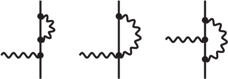
Figure 1: One-photon loop diagrams contributing to charge renormalization in scalar QED. Additional diagrams obtained by a horizontal reflection are not shown. A self-energy correction on an external line (left graph) brings $1/2$ of the pion wavefunction renormalization. In total the effects sum to zero.

3 Evaluation of one-photon loop diagrams

In this section, we present analytical results for the radiative corrections of order $\alpha$ to the invariant amplitudes $A(s,u)$ and $B(s,u)$ of pion Compton scattering. Our convenient choice of Coulomb gauge (in the center-of-mass frame) eliminates still all $s$-channel pole diagrams since for these either the initial state or final state photon coupling vanishes identically. Dropping also the diagrams with a tadpole-type self-energy insertion (the loop consisting of a single virtual photon line, which is set to zero in dimensional regularization) we are left with the 20 one-photon loop diagrams shown in Fig. 2. For the purpose of an ordering scheme they have been divided into classes I-XI. Due to an increasing number of internal pion propagators their evaluation rises in complexity. In order to simplify all calculations, we exploit gauge invariance and employ the Feynman gauge where the photon propagator is just proportional to the Minkowski metric tensor $g^{\mu\nu}$. Moreover, for a concise presentation of the one-loop amplitudes, $A(s,u)^{(\gamma-\rm loop)}$ and $B(s,u)^{(\gamma-\rm loop)}$, it is most helpful to work with the dimensionless kinematical variables $\hat{s}=s/m_{\pi}^{2}\geq 1$, $\hat{t}=t/m_{\pi}^{2}\leq 0$ and $\hat{u}=u/m_{\pi}^{2}\leq 1$, which obey the relation $\hat{s}+\hat{t}+\hat{u}=2$.

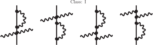
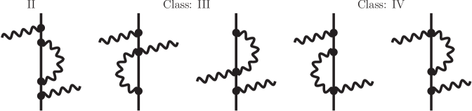
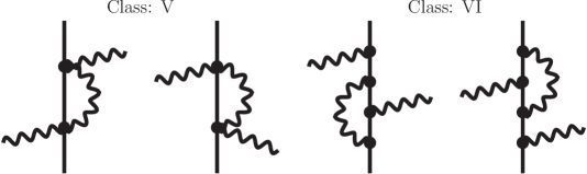
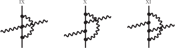
Figure 2: One-photon loop diagrams for radiative corrections to pion Compton scattering.

We can now enumerate the analytical expressions for the 11 classes of contributing one-photon loop diagrams. For notational simplicity we drop the arguments $s$ and $u$ of the invariant amplitudes $A(s,u)$ and $B(s,u)$, as well as a superscript indicating the class of diagrams.

Class I: For this class of diagrams the tree level amplitudes in eq.(2) get multiplied by the wavefunction renormalization factor of the pion:

$$A={\alpha\over\pi}\Big{(}\xi_{IR}-\xi_{UV}\Big{)}\,,\qquad B={\alpha\over\pi}\,{\hat{s}-1\over\hat{u}-1}\Big{(}\xi_{IR}-\xi_{UV}\Big{)}\,.$$ (7)

Class II: This $u$-channel pole diagram involves the once-subtracted (off-shell) self-energy of the pion:

$$A=0\,,\qquad B={\alpha\over 2\pi}\,{\hat{t}\over\hat{u}-1}\bigg{[}2\xi_{UV}-2+{\hat{u}+1\over\hat{u}}\ln(1-\hat{u})\bigg{]}\,.$$ (8)

Class III: These $u$-channel pole diagrams generate a constant vertex correction factor:

$$A=0\,,\qquad B={\alpha\over 2\pi}\,{\hat{t}\over\hat{u}-1}\bigg{[}-3\xi_{UV}+{7\over 2}\bigg{]}\,.$$ (9)

Class IV: These $u$-channel pole diagrams generate a $\hat{u}$-dependent vertex correction factor:

$$A=0\,,\qquad B={\alpha\over 2\pi}\,{\hat{t}\over\hat{u}-1}\bigg{[}-3\xi_{UV}+3+{1\over 2\hat{u}}+{1-\hat{u}\over 2\hat{u}^{2}}(3\hat{u}+1)\ln(1-\hat{u})\bigg{]}\,.$$ (10)

Class V: The sum of photon rescatterings in the $s$- and $u$-channel gives:

$$A=-B={\alpha\over 2\pi}\bigg{[}4\xi_{UV}-4+{\hat{s}-1\over\hat{s}}\ln(1-\hat{s})+{\hat{u}-1\over\hat{u}}\ln(1-\hat{u})\bigg{]}\,.$$ (11)

Class VI: These $u$-channel pole diagrams generate again a $\hat{u}$-dependent vertex correction factor:

$$A=0\,,\qquad B={\alpha\over 2\pi}\,{\hat{t}\over\hat{u}-1}\bigg{[}2\xi_{UV}-{5\over 2}-{1\over 2\hat{u}}-{\hat{u}^{2}+6\hat{u}+1\over 2\hat{u}^{2}}\ln(1-\hat{u})\bigg{]}\,,$$ (12)

Class VII: These irreducible $s$-channel diagrams give:

$$A=-B={\alpha\over 2\pi}\bigg{\{}-\xi_{UV}+{3\over 2}-{\hat{s}+1\over 2\hat{s}}\ln(1-\hat{s})+{1\over\hat{s}-1}\bigg{[}{\pi^{2}\over 6}-{\rm Li}_{2}(\hat{s})\bigg{]}\bigg{\}}\,,$$ (13)

where Li${}_{2}(x)=\sum_{n=1}^{\infty}n^{-2}x^{n}=x\int_{1}^{\infty}dy[y(y-x)]^{-1}\ln y$ denotes the conventional dilogarithmic function.

Class VIII: These irreducible $u$-channel diagrams give:

$$A={\alpha\over 2\pi}\bigg{\{}-\xi_{UV}+{3\over 2}-{\hat{u}+1\over 2\hat{u}}\ln(1-\hat{u})+{1\over\hat{u}-1}\bigg{[}{\pi^{2}\over 6}-{\rm Li}_{2}(\hat{u})\bigg{]}\bigg{\}}\,,$$ (14)

$$B=-A+{\alpha\over 2\pi}\,{\hat{t}\over\hat{u}-1}\bigg{\{}{3\hat{u}-1\over 2\hat{u}^{2}}\ln(1-\hat{u})-{\hat{u}+1\over 2\hat{u}}+{1\over\hat{u}-1}\bigg{[}{\rm Li}_{2}(\hat{u})-{\pi^{2}\over 6}\bigg{]}\bigg{\}}\,.$$ (15)

Class IX: The $t$-dependent vertex correction to the two-photon contact coupling reads:

$$A=-B\!\!\! = \!\!\!{\alpha\over 2\pi}\bigg{\{}-\xi_{UV}+1+\sqrt{4-\hat{t}}\,L(t)+{\hat{t}-2\over\sqrt{\hat{t}^{2}-4\hat{t}}}\bigg{[}4\xi_{IR}\sqrt{-\hat{t}}\,L(t)$$ (16)

$$\qquad+{\rm Li}_{2}(w)-{\rm Li}_{2}(1-w)+{1\over 2}\ln^{2}w-{1\over 2}\ln^{2}(1-w)\bigg{]}\bigg{\}}\,.$$

Here, we have introduced the frequently occurring logarithmic loop function:

$$L(t)={m_{\pi}\over\sqrt{-t}}\ln{\sqrt{4m_{\pi}^{2}-t}+\sqrt{-t}\over 2m_{\pi}}\,,$$ (17)

and the auxiliary variable $w$ appearing in eq.(16) is determined by the relation $1-2w=\sqrt{-t/(4m_{\pi}^{2}-t)}$.

Class X: The $s$-channel box diagram gives:

$$A\!\!\! = \!\!\!{\alpha\over 2\pi}\bigg{\{}{1\over 2}\xi_{UV}-{3\over 4}+{\hat{s}+1\over 2\hat{s}}\ln(1-\hat{s})+{1\over\hat{s}-1}\bigg{[}{\rm Li}_{2}(\hat{s})-{\pi^{2}\over 6}\bigg{]}-{1\over 2}\sqrt{4-\hat{t}}\,L(t)$$ (18)

$$-L^{2}(t)+\int_{1}^{\infty}\!\!{dx\over x-\hat{s}}\,{2-\hat{t}\over(x-1)^{2}+\hat{t}x}\Big{[}(x+1)\ln x+2(1-x)\sqrt{4-\hat{t}}\,L(t)\Big{]}\bigg{\}}\,,$$

$$B\!\!\! = \!\!\!-A+{\alpha\over 2\pi}\bigg{\{}{1\over 4}-L^{2}(t)+\int_{1}^{\infty}\!\!{dx\over x-\hat{s}}\,{2-\hat{t}\over[(x-1)^{2}+\hat{t}x]^{2}}\bigg{[}\hat{t}x(x+1)\ln x$$ (19)

$$+[(x-1)^{2}+\hat{t}x](x-1)+{2(x-1)\over\sqrt{4-\hat{t}}}[\hat{t}^{2}x-6\hat{t}x-2(x-1)^{2}]L(t)\bigg{]}\bigg{\}}\,.$$

The loop integrals involving four propagators are written here in terms of their spectral function representations (employing the Kramers-Kronig dispersion relation), where the $x$-dependent integrands stand for the corresponding imaginary parts. For the numerical evaluation of the relevant real parts of $A$ and $B$ one has to treat $\int_{1}^{\infty}dx/(x-\hat{s})\dots$ as a principal value integral. It can be conveniently decomposed into a sum of two nonsingular integrals by the following formula:

$$-\!\!\!\!\!\!\int_{1}^{\infty}\!\!dx\,{f(x)\over x-\hat{s}}=\int_{1}^{2\hat{s}-1}\!\!dx\,{f(x)-f(\hat{s})\over x-\hat{s}}+\int_{2\hat{s}-1}^{\infty}\!\!dx\,{f(x)\over x-\hat{s}}\,.$$ (20)

Class XI: The $u$-channel box diagram gives:

$$A\!\!\! = \!\!\!{\alpha\over 2\pi}\bigg{\{}{1\over 2}\xi_{UV}-{3\over 4}+{\hat{u}+1\over 2\hat{u}}\ln(1-\hat{u})+{1\over\hat{u}-1}\bigg{[}{\rm Li}_{2}(\hat{u})-{\pi^{2}\over 6}\bigg{]}-{1\over 2}\sqrt{4-\hat{t}}\,L(t)$$ (21)

$$-L^{2}(t)+\int_{1}^{\infty}\!\!{dx\over x-\hat{u}}\,{2-\hat{t}\over(x-1)^{2}+\hat{t}x}\Big{[}(x+1)\ln x+2(1-x)\sqrt{4-\hat{t}}\,L(t)\Big{]}\bigg{\}}\,,$$

$$B\!\!\! = \!\!\!-A+{\alpha\over 2\pi}\Bigg{\{}{\hat{t}(\hat{u}+1)\over 2\hat{u}(\hat{u}-1)}+{\hat{t}(1-\hat{u}-2\hat{u}^{2})\over 2\hat{u}^{2}(\hat{u}-1)}\ln(1-\hat{u})+{\hat{t}\over(\hat{u}-1)^{2}}\bigg{[}{\pi^{2}\over 6}-{\rm Li}_{2}(\hat{u})\bigg{]}$$ (22)

$$+{1\over 4}-L^{2}(t)+{\hat{t}^{2}-2\hat{t}\over(1-\hat{u})\sqrt{\hat{t}^{2}-4\hat{t}}}\bigg{[}4\Big{(}\xi_{IR}+\ln(1-\hat{u})\Big{)}\sqrt{-\hat{t}}\,L(t)+{\rm Li}_{2}(w)$$

$$-{\rm Li}_{2}(1-w)+{1\over 2}\ln^{2}w-{1\over 2}\ln^{2}(1-w)+{\rm Li}_{2}(h_{-})-{\rm Li}_{2}(h_{+})\bigg{]}+\int_{1}^{\infty}\!\!{dx\over x-\hat{u}}\,$$

$$\times{2-\hat{t}\over[(x-1)^{2}+\hat{t}x]^{2}}\bigg{\{}\hat{t}(x+1)(2-\hat{t}-x)\ln x+[(x-1)^{2}+\hat{t}x]\Big{(}x+\hat{t}+{\hat{t}\over x}-1\Big{)}$$

$$+{2L(t)\over\sqrt{4-\hat{t}}}\Big{[}\hat{t}^{3}(x+1)+\hat{t}^{2}(3x^{2}-3x-4)+2\hat{t}(x^{3}-4x^{2}+2x+1)-2(x-1)^{3}\Big{]}\bigg{\}}\Bigg{\}}\,,$$

where the arguments $h_{\pm}$ of the dilogarithms Li${}_{2}(h_{\pm})$ are determined by the relation $2m_{\pi}^{2}h_{\pm}=t\pm\sqrt{t^{2}-4m_{\pi}^{2}t}$.

Several checks of our calculation can be performed now. First, one verifies that the ultraviolet divergent terms proportional to $\xi_{UV}$ cancel in the total sums for $A$ and $B$ separately (using the relation $\hat{s}+\hat{u}+\hat{t}=2$ in the latter case). Secondly, crossing symmetry implies for our chosen set of independent amplitudes that $A(s,u)$ and $(u-m_{\pi}^{2})(s-m_{\pi}^{2})^{-1}B(s,u)$ are symmetric functions under the exchange of the variables, $s\leftrightarrow u$. This property follows e.g. by relating our set of amplitudes, $A(s,u)$ and $B(s,u)$ defined via eq.(1), to the (manifestly) crossing-symmetric functions introduced in refs.[4, 5]. While the symmetry condition $A(s,u)=A(u,s)$ becomes evident after summing up all contributions, the one for $B(s,u)$ provides a highly nontrivial check between analytical terms and terms represented by dispersion integrals in eqs.(18-22). In its consequence, crossing symmetry interrelates the whole set of one-loop diagrams in Fig. 2, which as such is not manifestly crossing-symmetric due to the particular choice of Coulomb gauge.

4 Infrared finiteness

In the next step we have to consider the infrared divergencies. Inspection of eqs.(7,16,22) reveals that the (summed) infrared divergent terms proportional to $\xi_{IR}$ appear in the same ratio $A(s,u):B(s,u)$ as the (tree level) Born terms written in eq.(2). As a consequence of that, the infrared divergent virtual (loop) corrections multiply the point-like cross section $d\sigma^{(\rm pt)}/d\Omega_{\rm cm}$ by a factor:

$$\delta_{\rm virt}^{(\rm IR)}={2\alpha\over\pi}\Bigg{[}1+{2\hat{t}-4\over\sqrt{4-\hat{t}}}L(t)\Bigg{]}\,\xi_{IR}\,.$$ (23)

The unphysical infrared divergence $\xi_{IR}$ gets canceled at the level of the cross section by the contributions of soft photon bremsstrahlung. In its final effect, the (single) soft photon radiation multiplies the tree level cross section $d\sigma^{(\rm pt)}/d\Omega_{\rm cm}$ by a (universal) factor [10, 13]:

$$\delta_{\rm soft}=\alpha\,\mu^{4-d}\!\!\int\limits_{|\vec{l}\,|<\lambda}\!\!{d^{d-1}l\over(2\pi)^{d-2}\,l_{0}}\bigg{\{}{2m_{\pi}^{2}-t\over p_{1}\cdot l\,p_{2}\cdot l}-{m_{\pi}^{2}\over(p_{1}\cdot l)^{2}}-{m_{\pi}^{2}\over(p_{2}\cdot l)^{2}}\bigg{\}}\,,$$ (24)

which depends on a small energy resolution $\lambda$. Working out this momentum space integral by the method of dimensional regularization (with $d>4$) one finds that the infrared divergent correction factor $\delta_{\rm virt}^{(\rm IR)}\sim\xi_{IR}$ gets removed and the following finite radiative correction factor remains:

$$\delta_{\rm real}={\alpha\over\pi}\Bigg{\{}\bigg{[}2+{4\hat{t}-8\over\sqrt{4-\hat{t}}}L(t)\bigg{]}\ln{m_{\pi}\over 2\lambda}+{\hat{s}+1\over\hat{s}-1}\ln\hat{s}+\int_{0}^{1/2}\!\!dy\,{(\hat{s}+1)(\hat{t}-2)\over W[1-\hat{t}y(1-y)]}\ln{\hat{s}+1+W\over\hat{s}+1-W}\Bigg{\}}\,,$$ (25)

with the abbreviation $W=\sqrt{(\hat{s}-1)^{2}+4\hat{s}\hat{t}y(1-y)}$. One can easily convince oneself that the radiative correction factor $\delta_{\rm real}$ vanishes in forward direction $t=0$. We note that the terms beyond the ones proportional to $\ln(m_{\pi}/2\lambda)$ are specific for the evaluation of the soft photon correction factor $\delta_{\rm soft}$ in eq.(24) in the center-of-mass frame. As it is written in eq.(25), $\delta_{\rm real}$ refers to an (idealized) experimental situation where all undetected soft photon radiation would fill in momentum space a small sphere of radius $\lambda$ in the center-of-mass frame. In a real experiment this region will be of different shape with no sharp boundaries due the detector efficiencies etc. Such additional (experiment specific) radiative corrections can be accounted for and calculated by integrating the fivefold differential cross section for $\pi^{-}\gamma\to\pi^{-}\gamma\gamma$ [9] over the appropriate region in phase space. By construction this region excludes the infrared singular domain $|\vec{l}\,|<\lambda$ and thus leads to a finite result.

We are now in the position to present numerical results for the radiative corrections to pion Compton scattering. The complete radiative correction factor is $\delta_{\rm real}$ written in eq.(25) plus all finite loop amplitudes $A$ and $B$ inserted into the interference cross section $d\sigma_{\rm int}/d\Omega_{\rm cm}$ and divided by the tree level cross section $d\sigma_{\rm pt}/d\Omega_{\rm cm}$. Fig. 3 shows in percent the total radiative correction factor for three selected center-of-mass energies $\sqrt{s}=(2,3,4)m_{\pi}$ as a function of $z=\cos\theta_{\rm cm}$. The detection threshold for soft photons has been set to the value $\lambda=5\,$MeV. One observes that the radiative corrections become maximal in backward directions $z\simeq-1$, reaching values up to $-2.4\%$ for $\sqrt{s}=4m_{\pi}$. With such an angular dependence the pure QED radiative corrections have the same kinematical signature as the effects from the pion’s low-energy structure (i.e. pion polarizability difference $\alpha_{\pi}-\beta_{\pi}$ and pion-loop correction of chiral perturbation theory [9]). In magnitude they are suppressed by about a factor $5-10$. We agree qualitatively with the findings of ref.[12] that the radiative corrections simulate effects of (fake) pion polarizabilities $\alpha_{\pi}^{(rc)}=-\beta_{\pi}^{(rc)}\simeq 3\cdot 10^{-5}\,$fm³ corresponding in magnitude to about $10\%$ of the prediction of chiral perturbation theory [5]. A proper inclusion of radiative corrections is therefore essential if one wants to extract the pion polarizabilities from Compton scattering data with good accuracy. We also note that when increasing the energy resolution scale $\lambda$ the magnitude of the radiative correction goes down. For example, with $\lambda=10\,$MeV or $20\,$MeV the before-mentioned $-2.4\%$ change to $-1.8\%$ or $-1.2\%$.

Finally, it is worth to mention that as one approaches (at fixed scattering angle $z=\cos\theta_{\rm cm}$) the Compton threshold, $\sqrt{s}\to m_{\pi}$, all radiative correction effects go away [11]. In this long-wavelength limit only the pure Thomson amplitude $T_{\pi\gamma}=-8\pi\alpha\,\vec{\epsilon}_{1}\cdot\vec{\epsilon}_{2}^{\,\,*}$ survives. This non-renormalization theorem is strictly fulfilled by the one-loop amplitudes $A(s,u)$ and $B(s,u)$ written in eqs.(7-22). In the same way, a direct computation at zero photon momentum $k_{1}=k_{2}=0$ gives for the factor multiplying the Thomson amplitude:

$$1+{\alpha\over 4\pi}\Big{[}(4\xi_{IR}-4\xi_{UV})^{\rm(I)}+(8\xi_{UV}-8)^{\rm(V)}+(1-2\xi_{UV})^{\rm(VII)}+(1-2\xi_{UV})^{\rm(VIII)}$$

$$\qquad\qquad+(4-4\xi_{IR}-2\xi_{UV})^{\rm(IX)}+(\xi_{UV}+1)^{\rm(X)}+(\xi_{UV}+1)^{\rm(XI)}\Big{]}\,,$$ (26)

where we have indicated the (classes of) contributing diagrams.

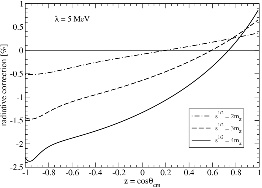
Figure 3: Radiative corrections for pion Compton scattering $\pi^{-}\gamma\to\pi^{-}\gamma$. The pion is treated as a structureless spin-0 boson.

5 Radiative corrections including pion polarizabilities

So far we have treated in our calculation of the radiative corrections the pion as a structureless spin-0 boson. Such an approximation is valid only at very low (photon) energies. The leading pion structure relevant for Compton scattering is given by the difference of its electric and magnetic polarizability $\alpha_{\pi}-\beta_{\pi}$. In an effective field theory approach it is easily accounted for by a new two-photon contact-vertex proportional to the squared electromagnetic field strength tensor, $F_{\mu\nu}F^{\mu\nu}=2(\vec{B}^{2}-\vec{E}^{2})$. The S-matrix insertion following from this (higher-order) gauge-invariant effective $\pi\pi\gamma\gamma$-vertex reads:

$$8\pi i\beta_{\pi}m_{\pi}\Big{(}k_{1}\cdot k_{2}\,\epsilon_{1}\cdot\epsilon^{*}_{2}-\epsilon_{1}\cdot k_{2}\,\epsilon^{*}_{2}\cdot k_{1}\Big{)}\,,$$ (27)

where one photon $(k_{1},\epsilon_{1})$ is ingoing and the other one $(k_{2},\epsilon_{2})$ outgoing. At tree level the polarizability vertex eq.(27) gives rise to the contributions $A(s,u)^{(\rm pola)}=-\beta_{\pi}m_{\pi}t/2\alpha$ and $B(s,u)^{(\rm pola)}=0$ to the invariant Compton scattering amplitudes. In order to prevent any misunderstandings we stress that when writing (merely) $\beta_{\pi}m_{\pi}$ for the coupling strength in eq.(27), an electric and a magnetic pion polarizability, equal in magnitude and opposite in sign $\alpha_{\pi}=-\beta_{\pi}$, are always both included.

We can reinterpret the one-photon loop diagrams in Fig. 2 now in such a way that the two-photon contact-vertex represents the polarizability vertex proportional to $\beta_{\pi}m_{\pi}$. In the case of class V we have to treat two cases, namely either the upper or lower contact-vertex. Going through the classes I, III-IX and reevaluating the loop diagrams with the S-matrix insertion from the polarizability vertex, we find the following contributions to the invariant amplitudes $A$ and $B$.

Class I:

$$A={\beta_{\pi}m_{\pi}\,t\over 2\pi}\Big{(}\xi_{UV}-\xi_{IR}\Big{)}\,,\qquad B=0\,,$$ (28)

Class V:

$$A={\beta_{\pi}m_{\pi}^{3}\over 2\pi}\bigg{[}-\xi_{UV}\,\hat{t}+\hat{t}+1-{1\over 2\hat{s}}-{1\over 2\hat{u}}+{(\hat{s}-1)^{3}\over 2\hat{s}^{2}}\ln(1-\hat{s})+{(\hat{u}-1)^{3}\over 2\hat{u}^{2}}\ln(1-\hat{u})\bigg{]}\,,$$ (29)

$$B=-A+{\beta_{\pi}m_{\pi}\,t\over 2\pi}\bigg{[}-\xi_{UV}+1-{1\over 2\hat{u}}-{(\hat{u}-1)^{2}\over 2\hat{u}^{2}}\ln(1-\hat{u})\bigg{]}\,,$$ (30)

Class VII:

$$A={\beta_{\pi}m_{\pi}^{3}\over 2\pi}(\hat{u}-1)\bigg{\{}\xi_{UV}-{3\over 2}+{\hat{s}+1\over 2\hat{s}}\ln(1-\hat{s})+{1\over\hat{s}-1}\bigg{[}{\rm Li}_{2}(\hat{s})-{\pi^{2}\over 6}\bigg{]}\bigg{\}}\,,$$ (31)

$$B={\hat{s}-1\over\hat{u}-1}\,A\,,$$ (32)

Class VIII:

$$A={\beta_{\pi}m_{\pi}^{3}\over 2\pi}(\hat{s}-1)\bigg{\{}\xi_{UV}-{3\over 2}+{\hat{u}+1\over 2\hat{u}}\ln(1-\hat{u})+{1\over\hat{u}-1}\bigg{[}{\rm Li}_{2}(\hat{u})-{\pi^{2}\over 6}\bigg{]}\bigg{\}}\,,$$ (33)

$$B=-A+{\beta_{\pi}m_{\pi}\,t\over 2\pi}\,{\hat{s}-1\over\hat{u}-1}\bigg{\{}{\hat{u}+1\over 2\hat{u}}+{1-3\hat{u}\over 2\hat{u}^{2}}\ln(1-\hat{u})+{1\over\hat{u}-1}\bigg{[}{\pi^{2}\over 6}-{\rm Li}_{2}(\hat{u})\bigg{]}\bigg{\}}\,,$$ (34)

Class IX:

$$A={\beta_{\pi}m_{\pi}\,t\over 4\pi}\bigg{\{}\xi_{UV}-1-\sqrt{4-\hat{t}}\,L(t)+{2-\hat{t}\over\sqrt{\hat{t}^{2}-4\hat{t}}}\bigg{[}4\xi_{IR}\sqrt{-\hat{t}}\,L(t)$$

$$\qquad+{\rm Li}_{2}(w)-{\rm Li}_{2}(1-w)+{1\over 2}\ln^{2}w-{1\over 2}\ln^{2}(1-w)\bigg{]}\bigg{\}}\,,\qquad B=0\,.$$ (35)

The contributions from classes III and IV (multiplicative vertex correction factors) vanish due to some special features of the S-matrix insertion eq.(27).

One verifies that the ultraviolet divergent terms proportional to $\xi_{UV}$ drop out in the total sum for $B(s,u)$, but not for $A(s,u)$. In the latter case the $t\,\xi_{UV}$-term can be canceled by interpreting the coupling constant in eq.(27) as a bare one and splitting it as $\beta_{\pi}^{(\rm bare)}=\beta_{\pi}(1-\alpha\,\xi_{UV}/2\pi)$ into the physical coupling constant $\beta_{\pi}$ and a counterterm piece. One also convinces oneself easily that the crossing-symmetry relations are fulfilled for the total sums of $A(s,u)$ and $B(s,u)$. The infrared divergent terms proportional to $\xi_{IR}$ showing up in eqs.(28,35) are again canceled by the soft photon bremsstrahlung contributions. As a result, one has to multiply the partial cross section linear in the polarizability:

$${d\sigma^{(\rm pola)}\over d\Omega_{\rm cm}}={\alpha\beta_{\pi}m_{\pi}^{3}(s-m_{\pi}^{2})^{2}(1-z)^{2}\over 2s^{2}[s(1+z)+m_{\pi}^{2}(1-z)]}\,,$$ (36)

with the radiative correction factor $\delta_{\rm real}$ written down in eq.(25).

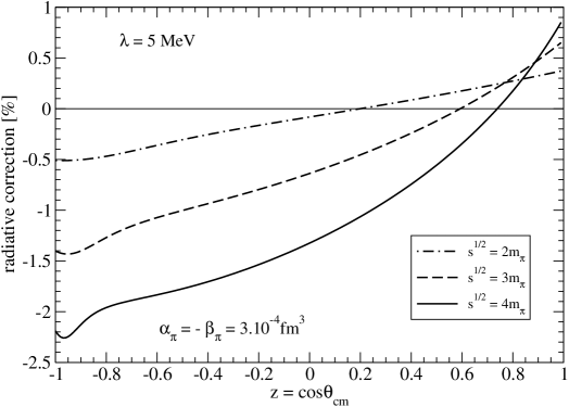
Figure 4: Radiative corrections for pion Compton scattering $\pi^{-}\gamma\to\pi^{-}\gamma$. The pion’s low-energy structure is included through a polarizability difference $\alpha_{\pi}-\beta_{\pi}\simeq 6\cdot 10^{-4}\,$fm³.

In Fig. 4 we show again the radiative correction factor for center-of-mass energies $\sqrt{s}=(2,3,4)m_{\pi}$ as a function of $z=\cos\theta_{\rm cm}$ with a pion polarizability difference of $\alpha_{\pi}-\beta_{\pi}\simeq 6\cdot 10^{-4}\,$fm³ included. The reference cross section is now the sum ${d\sigma^{(\rm pt)}/d\Omega_{\rm cm}}+{d\sigma^{(\rm pola)}/d\Omega_{\rm cm}}$ of point-like and polarizability-improved ($\sim\beta_{\pi}$) cross section. The radiative correction is of course for each part of relative order $\alpha$. The detection threshold of soft photons has been kept at the value $\lambda=5\,$MeV. In comparison to Fig. 3 one observes almost no changes for the three curves in Fig. 4. Only some slight upward shifts of the maximal values near $z\simeq-1$ are visible. We can therefore conclude that the size and angular dependence of the radiative corrections to pion Compton scattering remain practically unchanged when including the leading structure effect in form of the pion polarizability difference $\alpha_{\pi}-\beta_{\pi}\simeq 6\cdot 10^{-4}\,$fm³. Of course, there is yet the pion-loop correction of chiral perturbation theory [4, 5]. In the cross sections it works partly against the polarizability effects [9]. It is expected that the combined radiative pion-photon two-loop corrections (emerging from a vast number of two-loop diagrams) will follow the same trend.

In summary, we have presented a detailed (analytical) calculation of radiative corrections to pion Compton scattering which can be utilized for data analyses.

Appendix: Cross section for pion-nucleus bremsstrahlung

It is common practice to extract from Primakoff events in high-energy pion-nucleus bremsstrah- lung a cross section for pion Compton scattering via the equivalent photon method [14]. This involves a kinematical extrapolation from (time-like polarized) virtual photons to (space-like transverse) real photons. While the procedure becomes exact for asymptotically small photon virtualities $q^{2}\to 0$, it introduced uncertainties into the analysis of real experiments, where only some lower bounds can be reached. Moreover, at the very low photon-virtualities $q^{2}$ shielding effects of the nuclear charge by inner-shell atomic electrons comes into play as a further complication. The issue of Coulomb-strong interaction interference in pion-nucleus bremsstrahlung has been studied recently in ref.[15]. According to this work it is advantageous to restrict oneself to momentum transfers $|\vec{q}\,|\leq 32\,$MeV $\simeq m_{\pi}/4$, since there the ratio between polarizability and Born contributions remains essentially the same as for real pion Compton scattering.

We want to point out here, that for the purpose of determining the pion polarizabilities (i.e. the dominant difference $\alpha_{\pi}-\beta_{\pi}$) one can omit the whole extrapolation procedure and directly analyze the pion bremsstrahlung process as it is measured in the laboratory frame. The relevant ingredients to the cross section (at sufficiently low momentum transfers $|\vec{q}\,|$ where the one-photon exchange dominates) are summarized in this appendix.

Consider the pion bremsstrahlung process, $\pi^{-}(\vec{p}_{1})+Z_{\rm rest}\to\pi^{-}(\vec{p}_{2})+\gamma(\vec{k},\vec{\epsilon}\,)+Z_{\rm recoil}$, where a virtual photon transfers the (small) momentum $\vec{q}=\vec{p}_{2}+\vec{k}-\vec{p}_{1}$ from the nucleus (of charge $Z$) to the pion. The extremely small recoil energy $-q_{0}=\vec{q}\,^{2}/2M_{\rm nucl}\approx 0$ of the nucleus can be neglected. The fivefold differential cross section in the laboratory frame reads [16]:

$${d^{5}\sigma\over d\omega d\Omega_{\gamma}d\Omega_{\pi}}={Z^{2}\alpha^{3}\omega p_{2}\over\pi^{2}p_{1}q^{4}}\,H\,,$$ (37)

with $q=|\vec{q}\,|$ and $H$ the squared amplitude summed over the final state photon polarizations $(\vec{\epsilon}\cdot\vec{k}=0)$:

$$H=(\tilde{A}p_{1}\sin\theta_{1})^{2}+(\tilde{B}p_{2}\sin\theta_{2})^{2}+2\tilde{A}\tilde{B}p_{1}p_{2}\sin\theta_{1}\sin\theta_{2}\cos\phi\,.$$ (38)

This expression has been derived from a T-matrix for the virtual Compton scattering process, $\pi^{-}\gamma^{*}\to\pi^{-}\gamma$, of the form $T=-8\pi\alpha(\tilde{A}\,\vec{\epsilon}\,^{*}\cdot\vec{p}_{1}+\tilde{B}\,\vec{\epsilon}\,^{*}\cdot\vec{p}_{2})$ with $\tilde{A}$ and $\tilde{B}$ two (real) amplitudes. $\theta_{1}$ and $\theta_{2}$ are the angles between the momentum vectors $\vec{k}$ and $\vec{p}_{1}$ and $\vec{p}_{2}$, respectively. In addition, $\phi$ is the angle between the two planes spanned by $(\vec{k},\vec{p}_{1})$ and $(\vec{k},\vec{p}_{2})$.

The (three) tree diagrams of scalar quantum electrodynamics lead to the following contributions to the amplitudes $\tilde{A}$ and $\tilde{B}$:

$$\tilde{A}^{(\rm tree)}={E_{2}\over\omega(E_{1}-p_{1}\cos\theta_{1})}\,,\qquad\tilde{B}^{(\rm tree)}={-E_{1}\over\omega(E_{2}-p_{2}\cos\theta_{2})}\,,$$ (39)

with $E_{1}=\sqrt{p_{1}^{2}+m_{\pi}^{2}}$ the initial energy of the pion, $E_{2}=E_{1}-\omega$ the final energy of the pion and $p_{2}=\sqrt{p_{1}^{2}-2E_{1}\omega+\omega^{2}}$. The photon energy is denoted by $\omega$. Note that the diagram involving the two-photon contact-vertex of scalar QED vanishes here, due to the orthogonality of the time-like virtual photon and the space-like real photon polarizations, $\epsilon_{0}=0$. The contributions from the pion electric and magnetic polarizabilities (taking $\alpha_{\pi}=-\beta_{\pi}$ as a good approximation) read:

$$\tilde{A}^{(\rm pola)}=-\tilde{B}^{(\rm pola)}={\beta_{\pi}m_{\pi}\omega\over\alpha}\,.$$ (40)

It follows directly from the S-matrix insertion in eq.(27) evaluated in the present kinematical situation, $\pi^{-}\gamma^{*}\to\pi^{-}\gamma$. At the same order (in the small momentum expansion) there are the pion-loop corrections of chiral perturbation theory [17]. On the one hand side, they introduce the charge form factor of the pion:

$$F_{\pi}(q^{2})=1-{q^{2}\over 6}\langle r^{2}_{\pi}\rangle+{1\over 12\pi^{2}f_{\pi}^{2}}\bigg{\{}-m_{\pi}^{2}-{q^{2}\over 3}+{(4m_{\pi}^{2}+q^{2})^{3/2}\over 4q}\tilde{L}(q)\bigg{\}}\,,$$ (41)

with $\langle r^{2}_{\pi}\rangle=(0.45\pm 0.01)$ fm² [18] the mean square charge radius of the pion, $f_{\pi}=92.4\,$MeV the pion decay constant, and the logarithmic loop function:

$$\tilde{L}(q)=\ln{\sqrt{4m_{\pi}^{2}+q^{2}}+q\over 2m_{\pi}}\,.$$ (42)

Figure 5: Loop diagram for virtual pion Compton scattering.

As a result, the tree level Born terms, $\tilde{A}^{(\rm tree)}$ and $\tilde{B}^{(\rm tree)}$ in eq.(39), have then to be multiplied by the pion charge form factor $F_{\pi}(q^{2})$, because a virtual photon (with $q^{2}\neq 0$) coupling to the pion can resolve this part of structure of the pion. Moreover and specific for (virtual) Compton scattering, there is the pion-loop diagram shown in Fig. 5. It describes photon scattering off the ”pion-cloud around the pion” and leads to the following contribution [17]:

$$\tilde{A}^{(\rm loop)}=-\tilde{B}^{(\rm loop)} = {\omega\tau^{2}\over(4\pi f_{\pi})^{2}(\tau^{2}-q^{2})^{2}}\bigg{\{}\tau^{2}-q^{2}+4m_{\pi}^{2}\Big{[}\tilde{L}^{2}(q)-\tilde{L}^{2}(\tau)\Big{]}$$ (43)

$$+2q\sqrt{4m_{\pi}^{2}+q^{2}}\,\tilde{L}(q)-{2q^{2}\over\tau}\sqrt{4m_{\pi}^{2}+\tau^{2}}\,\tilde{L}(\tau)\bigg{\}}\,.$$

Note that this irreducible loop contribution depends on both, the photon virtuality $q^{2}$ and the squared invariant momentum transfer $-\tau^{2}$ between the initial and final state pion, with $\tau^{2}=\vec{q}\cdot(\vec{q}-2\vec{k}\,)=(\vec{p}_{1}-\vec{p}_{2})^{2}-\omega^{2}$ where $\vec{p}_{1}\cdot\vec{p}_{2}=p_{1}p_{2}(\cos\theta_{1}\cos\theta_{2}+\sin\theta_{1}\sin\theta_{2}\cos\phi)$. In the cross section, the pion-loop correction in eq.(43) compensates in part the effects from the pion polarizabilities [9]. Therefore, it is important to include it in the analysis of pion bremsstrahlung data, if one wants to extract reliably the pion polarizability difference $\alpha_{\pi}-\beta_{\pi}$.

Of course, there are yet the one-photon loop radiative corrections to virtual pion Compton scattering $\pi^{-}\gamma^{*}\to\pi^{-}\gamma$ (see Fig. 2). These will be presented (in the same style as done here for real pion Compton scattering) in a forthcoming publication [19].

References

- [1] M.V. Terentev, Sov. J. Nucl. Phys. 16, 87 (1973).
- [2] E. Frlez et al., Phys. Rev. Lett. 93, 181804 (2004); hep-ex/0606023.
- [3] J.F. Donoghue and B.R. Holstein, Phys. Rev. D40, 2378 (1989).
- [4] U. Bürgi, Phys. Lett. B377, 147 (1996); Nucl. Phys. B479, 392 (1996).
- [5] J. Gasser, M.A. Ivanov, and M.E. Sainio, Nucl. Phys. B745, 84 (2006); and refs. therein.
- [6] Y.M. Antipov et al., Phys. Lett. B121, 445 (1983); Z. Phys. C26, 495 (1985).
- [7] J. Ahrens et al., Eur. Phys. J. A23, 113 (2005).
- [8] COMPASS Collaboration: P. Abbon et al., hep-ex/0703049.
- [9] N. Kaiser and J.M. Friedrich, Eur. Phys. J. A36, 181 (2008).
- [10] L.M. Brown and R.P. Feynman, Phys. Rev. 85, 231 (1952).
- [11] E. Corinaldesi and R. Jost, Helv. Phys. Acta 21, 183 (1948).
-
[12]
A.A. Akhundov, D.Y. Bardin, and G.V. Mitselmakher,
Sov. J. Nucl. Phys. 37, 217 (1983);
A.A. Akhundov, D.Y. Bardin, G.V. Mitselmakher, and A.G. Olshevskii, Sov. J. Nucl. Phys. 42, 426 (1985);
A.A. Akhundov, S. Gerzon, S. Kananov, and M.A. Moinester, Z. Phys. C66, 279 (1995). - [13] M. Vanderhaeghen et al., Phys. Rev. C62, 025501 (2000); and refs. therein.
- [14] I.Y. Pomeranchuk and I.M. Shmushkevich, Nucl. Phys. 23, 452 (1961).
- [15] G. Fäldt and U. Tengblad, nucl-th/0807.2700; nucl-th/0802.0971; Phys. Rev. C76, 064607 (2007).
- [16] C. Itzykson and J.B. Zuber, Quantum Field Theory, McGraw-Hill book company, 1980; chapter 5.2.4.
- [17] C. Unkmeir, S. Scherer, A.I. Lvov, and D. Drechsel, Phys. Rev. C61, 034002 (2000).
- [18] Particle Data Group (W.M. Yao et al.), J. Phys. G33, 1 (2006).
- [19] N. Kaiser and J.M. Friedrich, in preparation.