Non-parametric strong lens inversion of Cl 0024+1654: illustrating the monopole degeneracy

Abstract

The cluster lens Cl 0024+1654 is undoubtedly one of the most beautiful examples of strong gravitational lensing, providing five large images of a single source with well-resolved substructure. Using the information contained in the positions and the shapes of the images, combined with the null space information, a non-parametric technique is used to infer the strong lensing mass map of the central region of this cluster. This yields a strong lensing mass of $1.60\times 10^{14}M_{\odot}$ within a 0.5^′ radius around the cluster center. This mass distribution is then used as a case study of the monopole degeneracy, which may be one of the most important degeneracies in gravitational lensing studies and which is extremely hard to break. We illustrate the monopole degeneracy by adding circularly symmetric density distributions with zero total mass to the original mass map of Cl 0024+1654. These redistribute mass in certain areas of the mass map without affecting the observed images in any way. We show that the monopole degeneracy and the mass-sheet degeneracy together lie at the heart of the discrepancies between different gravitational lens reconstructions that can be found in the literature for a given object, and that many images/sources, with an overall high image density in the lens plane, are required to construct an accurate, high-resolution mass map based on strong-lensing data.

1 Introduction

Due to the gravitational deflection of light, a galaxy or cluster of galaxies can affect the light that we receive from background sources. On larger scales, this leads to slight deformations of the shapes of the background sources, but close to the center of the deflecting object, the gravitational lens, more elaborate deformations are possible. When a background source is sufficiently well aligned with the gravitational lens, this strong lens effect can even cause multiple images of said source to appear. One of the most spectacular examples of strong gravitational lensing can be seen in the cluster lens Cl 0024+1654. Using recent ACS observations, one can easily see that five well resolved images depict a single source, but even before these five images were identified, it was clear that three arc segments were caused by a gravitational lens effect (Koo, 1988).

This strong lensing information was first used in Kassiola et al. (1992). The authors of this work noted that these arc segments do not obey the so-called length theorem (Kovner, 1990), implying that no simple elliptical lens model can be used. They show that if perturbations by cluster members are added, the observed arc lengths can indeed be reconstructed. In Wallington et al. (1995), a more advanced reconstruction technique was used, consisting of a smooth lens model perturbed by some smaller galaxies and a non-parametric source model. Whereas previous work suggested that the main cluster potential was offset from the largest galaxy, these authors find that these positions, in fact, agree well.

After the first HST images clearly revealed the presence of five images, more lensing studies followed. The new, well resolved images were used in Colley et al. (1996) to study the source itself, a blue galaxy containing some interesting dark features and a bar-like structure. Tyson et al. (1998) use the images to find the parameters describing elaborate lens and source models. Their algorithm constructs the complete image plane based on a set of source and lens parameters and compares the result with the HST observations. They find that the mass distribution is dominated by a smooth dark matter component with a considerable core radius, centered at a position near the largest cluster member.

Much of the earlier mass uncertainties originated from the poorly established source redshift. Broadhurst et al. (2000) finally measured a spectroscopic redshift of 1.675 and used this information in their own inversion. They found that the image positions can be accurately reproduced using a model which traces the locations of the brightest cluster members. In Jee et al. (2007), a non-parametric method is used to invert the lens, using both strong and weak-lensing data. In the strong lensing region, the retrieved mass profile closely resembles the result of Broadhurst et al. (2000), but according to Shapiro & Iliev (2000), the associated velocity dispersion is too high to correspond to the measured value of 1150 km s^-1 (Dressler et al., 1999).

In the present paper, we employ a non-parametric method to infer the mass map of Cl 0024+1654. This is the first time that only the information about the images themselves as well as the null space – i.e. the region where no images are observed – is used to reconstruct the mass distribution of this cluster in the strong lensing region. No information about the positions of cluster members is used. Clearly, many other possibilities have already been presented in the past, but it is not our intention to add to the confusion. Instead, the reconstruction is used to explain how the different previous inversions are related to each other.

Below, we will first briefly review the non-parametric technique that is worked out in detail in previous articles. In section 3 this method is applied to reconstruct the mass distribution of Cl 0024+1654, and this result is used in section 4 to illustrate the importance of the monopole degeneracy. The implications of these observations are discussed in section 5.

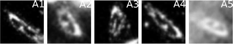
Figure 1: The image parts of the five images of source A which were used in the reconstruction, labeled in the same way as in the work of Jee et al. (2007). Due to the extended nature of these images, several corresponding features are easily identified. The images shown here are not displayed on the same scale.

Figure 2: Left panel: after averaging 28 individual reconstructions, this is the resulting mass map for Cl 0024+1654 predicted by our procedure. The positions of the input images of source A are also indicated in this figure. The critical density used in this figure corresponds to a redshift $z=3$. Right panel: the standard deviation of the individual reconstructions shows that the different solutions tend to disagree about the exact shape in the central part of the mass distribution. In particular, this figure suggests that the mass peak around $(0.2^{\prime},-0.2^{\prime})$ in the left panel should not be regarded as an actual feature.

2 Inversion method

Below we shall briefly describe a minor variation of the inversion method described in Liesenborgs et al. (2006) and Liesenborgs et al. (2007). The interested reader is referred to these works for a detailed description of the steps involved. A basic knowledge of gravitational lensing is assumed; we refer to Schneider et al. (1992) for an in-depth treatment of the subject.

2.1 Multi-objective genetic algorithms

A genetic algorithm is an optimization strategy in which one tries to produce acceptable solutions to an – often high-dimensional – problem using a mechanism inspired by natural selection. In effect, one tries to breed solutions to a problem.

One starts with a so-called population of genomes, each one encoding a trial solution to the problem. Based on this population, a new one is created by combining and mutating existing genomes. It is important to apply some kind of selection pressure: genomes which are deemed more fit should have a better chance of creating offspring. If only one fitness measure is needed, this selection mechanism can be implemented by first sorting the genomes in a population according to their fitness and by letting the selection probability depend on the position of the genome in this sorted population.

A similar approach can be used when more than one fitness measure should be optimized. One genome is said to dominate another one if it is at least as good with respect to each fitness criterion and if it is strictly better regarding at least one criterion. Using this concept of dominance, one can identify in a population the genomes which are not dominated by any other genome: the non-dominated set. These genomes should receive the highest selection probability. If one removes this set from the population, one can find a new non-dominated set which should receive the second-to-highest selection probability, etc.

For more information about both single- and multi-objective genetic algorithms, the interested reader is referred to Deb (2001).

2.2 Dynamic grid

At the start of the inversion procedure, the user is required to specify a square-shaped area in which the procedure should try to reconstruct the projected mass distribution. First, this region is subdivided uniformly into a number of smaller square grid cells, and to each grid cell, a projected Plummer sphere (Plummer, 1911) is associated. The widths of these basis functions are proportional to the sizes of the grid cells. Based on previous work, we use a Plummer width that is 1.7 times as large as the size of a cell.

Using a multi-objective genetic algorithm, the inversion procedure then tries to find weights for these basis functions which are compatible with the observed gravitational lensing scenario. Once these are found, the corresponding estimation of the mass distribution is used to create a new grid, with smaller grid cells in regions containing more mass. Plummer basis functions are again associated to each grid cell, and the genetic algorithm will try to find new values for their weights. This refinement procedure can be repeated a number of times, until an acceptable reconstruction is retrieved. Below we explain further which measures are used to determine if a solution is acceptable. This dynamic grid system is also used in Diego et al. (2005).

2.3 Fitness measures

If the true mass distribution were known, the corresponding lens equation would project each image of a single source onto the same region of the source plane. For this reason, the first fitness criterion measures the amount of overlap when images are projected onto their source planes by a trial solution. Each back-projected image provides an estimate of the shape of the source and determines a typical scale in the source plane. By averaging these scales over all the images of a single source, one obtains a final estimate of a typical scale for this source. In the original procedure, the back-projected images were surrounded by rectangles and the distances between corresponding corners – measured relative to the estimated size of the source – were used to calculate a measure for the overlap of the images. For the case of Cl 0024+1654, a small variation is used: because the images are well resolved, several matching points can be found in the images. The distances – still relative to the estimated source size – between these points when projected onto the source plane, are then used to calculate a measure for the overlap between the images.

Not only should the back-projected images form a consistent source, a candidate solution should also avoid predicting images where none are observed. A second fitness measure is included to avoid producing these kinds of solutions. To do so, the region where no images are observed – the null space – is subdivided into a number of small triangles. Each triangle is projected back onto the source plane and is compared to the current estimate of the source shape. For a specific trial solution, the shape of a source is estimated by projecting all image points onto the source plane, and by calculating the envelope of these points. If such a null-space triangle and the estimated source shape overlap, this would indicate that an extra image is predicted by the current trial solution. Such a comparison is done for each null-space triangle and the total amount of overlap with the source is used to calculate a fitness measure.

In the case of non-merging images, one would like to avoid critical lines intersecting the images. To do so, a third fitness criterion is used. It is easy to detect if a critical line intersects an image: one simply needs to calculate the sign of the magnification at each image point. Only if this is the same for all image points, no critical line intersects the image. In practice, the magnification signs of neighbouring points are compared and the fitness measure simply counts the number of pairs for which the signs change.

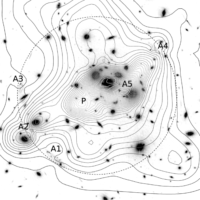
Figure 3: The contours of the retrieved mass map in the left panel of Fig. 2 are shown on top of the ACS image of the central cluster region (north is up, east is left). The lensing mass is found to be concentrated around the largest cluster galaxy and the central image A5 is found to be located between two mass peaks, which also resembles the observed situation. The positions of the two galaxies in the south-east region are retrieved very accurately as well. Note that this image also suggests that there is a density peak labeled P in a region where very few cluster light originates. The total mass in the region bounded by the dotted line is found to be $1.60\times 10^{14}M_{\odot}$. The area displayed in this figure is approximately 1.3^′ $\times$ 1.3^′.

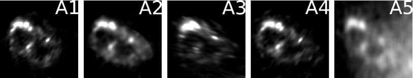
Figure 4: When the images shown in Fig. 1 are projected back onto the source plane, these source shapes are retrieved. Each figure shows the same region in the source plane, approximately 3^′′ by 3^′′ in size.

Figure 5: Left panel: this figure shows the predicted position of source A and B as well as the caustics corresponding to the redshift of source A. Source B is enclosed by a small square. Right panel: when the sources of the left panel are projected onto their image planes, these image positions arise. The image of source B which is closest to the origin was not part of the input; the model predicts an image at this location. Other than this image, no additional images were predicted.

2.4 Finalizing and averaging

The dynamic grid method has one disadvantage: regions containing only a relatively small portion of the total mass will not be subdivided into smaller grid cells. As a result, the basis functions in such regions may lack the resolution needed for an accurate reconstruction. To overcome this problem, a finalizing step was added to the procedure. A uniform grid of 64 by 64 grid cells was created and the associated basis functions are used as small corrections to the current estimate of the mass distribution. Because they are corrections, the weights of the basis functions are allowed to be negative. The genetic algorithm again determines appropriate values for these weights.

To create a single candidate solution, first the dynamic grid method is used to create a first good estimate of the mass distribution and afterwards, small-scale corrections are introduced in the finalizing step. This entire procedure is then repeated a number of times, each time yielding a somewhat different mass distribution. One can then calculate the average mass distribution to inspect the features which are common in all reconstructions, and one can calculate the standard deviation to check in which regions the individual solutions disagree.

3 Inverting Cl 0024+1654

3.1 Input

The inversion procedure described above, was applied to the cluster lens Cl 0024+1654. We use the images of sources A and B as described in Jee et al. (2007), at redshifts of 1.675 and 1.3 respectively. The redshift of the lens itself is 0.395 and angular diameter distances were calculated in a flat cosmological model with $H_{0}=71$ km s^-1 Mpc^-1, $\Omega_{m}=0.27$ and $\Omega_{\Lambda}=0.73$. The inversion procedure constructs the lensing mass distribution in a square shaped area of 1.3^′ by 1.3^′, centered on the brightest cluster galaxy. To avoid predicting images which are located relatively far away, the null space grid measured 3^′ by 3^′, centered on the same galaxy. Initially, a uniform grid of 15$\times$15 is used to place the Plummer basis functions on, and the grid is refined until approximately 800 basis functions are used. After this, the finalizing step is executed on a uniform 64$\times$64 grid. Below we shall see that this leads to a very good source reconstruction.

The gravitational lens creates several large images of source A, a blue galaxy. A part of the source is mapped onto five easily identifiable sub-images, as can be seen in Fig. 1. The high resolution ACS images allow several corresponding features to be identified (up to twelve features in some images), which will be used to calculate how well the back-projected images overlap. It is assumed that no other images of the source are present, so that only the five images themselves are excluded from the null space for this source. Source B only has two images, the third one most likely being occluded by the central cluster members. The complete images are used to estimate the source size, but only a single point in each image is used to measure how well the images overlap when projected back onto the source plane (measured relative to the estimated size of the source). In this case, not only the images themselves were excluded from the null space, but also the region in which the central cluster members reside. This allows the algorithm to predict an unobserved third image anywhere in that region. For both sources it is assumed that no critical lines intersect the images which are used.

3.2 Results

Using the inversion procedure described in section 2, the mass map shown in the left panel of Fig. 2 was obtained after averaging 28 individual solutions. This number is dictated by the computer time it takes to generate the individual solutions and by the fact that after averaging together 15 solutions or more, the average solution does not change significantly. The largest fraction of the rather steep mass distribution coincides with the position of the central cluster members. The central image of source A is located between two density peaks, which resembles the situation shown in the ACS images. These facts can be clearly seen when the retrieved mass contours are drawn on top of the observed situation, as is shown in Fig. 3. This same figures also illustrates the remarkable accuracy with which the two cluster galaxies enclosing the image at $(0.5^{\prime},-0.3^{\prime})$ are retrieved. We would like to stress again that these were retrieved automatically; no prior information about the presence of these galaxies was used. It is these galaxies that cause the middle image of the three arc segments to be compressed, thereby causing the violation of the length theorem. The mass inside a circular region of radius 0.5^′, centered on $(0.075^{\prime},-0.075^{\prime})$ is found to be $1.60\times 10^{14}M_{\odot}$. This region is enclosed by a dotted line in Fig. 3.

When the input images of source A are projected back onto the source plane, a consistent source is produced, as can be clearly seen in Fig. 4. The size of the source is approximately 2.5^′′ (corresponding to 21 kpc). This is larger than both the value of 1^′′ mentioned in Colley et al. (1996) and the value of 0.5^′′ mentioned in Jee et al. (2007), but the general appearance does agree very well with both works. We shall come back to this size difference later in section 5. The retrieved source positions and caustics at $z=1.675$ are depicted in the left panel of Fig. 5. If these sources are used to calculate the image positions, the results shown in the right panel of Fig. 5 are retrieved. From this image it is clear that the multi-objective genetic algorithm succeeded in generating solutions which only predict one extra image (for source B) and which do not have critical lines intersecting the input images.

Figure 6: Left panel: shape of the total mass map of the circularly symmetric basis functions used to construct degenerate solutions (see text). The value of $m$ determines the position of the maximum. Right panel: the total mass profiles shown in the left panel give rise to these density profiles. As the value of $m$ becomes smaller, the amplitude of the negative density part decreases.

On closer inspection of the resulting mass map in Fig. 2, there seems to be an intriguing feature at $(0.2^{\prime},-0.2^{\prime})$. At this location the mass map shows a clear peak, but in the ACS images no cluster member can be seen at this location (Fig. 3). Could this be evidence of dark matter in this cluster? Inspecting the standard deviation of the individual solutions helps to shed some light on this matter. As can be seen in the right panel of Fig. 2, the individual solutions do not agree well on the exact shape of the central part of the mass distribution. In fact, the largest uncertainty is located precisely around the position of this mysterious peak, which suggests that we should be very careful when trying to interpret this feature.

4 The monopole degeneracy

To verify if any particular feature can be regarded as a real feature of the mass map, a question one can ask is the following: can this feature be removed from the reconstruction while still obtaining a good inversion, given the available constraints? Below, we shall describe how the monopole degeneracy can help to answer this question and we shall apply it to the case of Cl 0024+1654.

For a circularly symmetric mass distribution $\Sigma(\theta)$, the expression for the bending angle in the lens plane simplifies to

$$\mbox{\boldmath$\hat{\alpha}$}(\mbox{\boldmath$\theta$})=\frac{4GM(\theta)}{c^{2}D_{\rm d}\theta^{2}}\mbox{\boldmath$\theta$}\mathrm{,}$$ (1)

in which $M(\theta)$ is the total mass enclosed within an angle $\theta$ from the center of this mass distribution:

$$M(\theta)=2\pi D_{\rm d}^{2}\int_{0}^{\theta}\Sigma(\theta^{\prime})\theta^{\prime}d\theta^{\prime}\mathrm{,}$$ (2)

and $D_{\rm d}$ is the angular diameter distance between lens and observer. From equation (1), it is clear that a circularly symmetric mass distribution of which the total mass is zero beyond a specific radius, does not produce a gravitational lens effect outside said radius. If such a mass distribution is added to an existing one, the original lens equation will be modified only inside the circular region in which it has non-zero mass.

Consider a lens mass map $M(x)$ specified by $M_{A}(x)$ in $[0,m]$, by $M_{B}(x)$ in $[m,1]$ and which is zero beyond the unit radius:

$$M_{A}(x) = -\frac{1}{4m^{2}}x^{4}+\frac{1}{2}x^{2}$$ (3)

$$M_{B}(x) = \frac{m^{2}}{4(m-1)^{3}}\times$$ (4)

$$\left[-2x^{3}+3(m+1)x^{2}-6mx+3m-1\right]\mathrm{.}$$

The shape of such a function is shown in the left panel of Fig. 6 for two different values of $m$, which specifies the position of the maximum. The right panel of the same figure shows the associated density profiles, which are composed of two parts as well:

$$\Sigma_{A}(x) = \frac{1}{x}\frac{dM_{A}}{dx}=-\frac{1}{m^{2}}x^{2}+1$$ (5)

$$\Sigma_{B}(x) = \frac{1}{x}\frac{dM_{B}}{dx}$$ (6)

$$= \frac{m^{2}}{4(m-1)^{3}}\left[-6x+6(m+1)-\frac{6m}{x}\right]\mathrm{.}$$

Clearly, the smaller the value of $m$, the flatter the density profile becomes after this point. Using such a profile, it is possible to introduce or erase a peak in an existing mass map without changing much to the rest of the distribution and while conserving the total mass.

Using basis functions of this type, we can build a more complex mass distribution that, when added to an existing gravitational lens reconstruction, will produce an equally acceptable solution. To do so, the region of interest is subdivided into a number of square-shaped grid cells. For each grid cell, the distance from its center to the nearest image is calculated. If this distance is relatively large compared to the size of the grid cell – e.g. at least four times as large – a basis function is associated to this cell. The distance to the nearest image is used as the unit length; the width of the non-negative part $\Sigma_{A}$ is set proportional to the size of the grid cell. This implies that for a specific basis function, all the images lie in the area within which the total mass of the basis function is zero. Since the lens equation for a circularly symmetric basis function only depends on the total mass within a specific radius, in this case the lens equation at the position of the images will be unaffected when such a basis function is added to the existing mass distribution. The property that the total mass of the basis function outside a certain radius is zero, is clearly an essential feature in this approach. Similarly, when all the basis functions on the grid are considered, the lens equation at the location of the images will not be influenced, independent of the precise weight values of the basis functions. Everywhere else, the lens equation will indeed be modified, meaning that extra images may be predicted, depending on the precise weight values used.

Figure 7: Left panel: if the grid based method to redistribute mass is applied to the mass map shown in the left panel of Fig. 2, this new distribution is obtained. The peak at $(0.2^{\prime},-0.2^{\prime})$ has automatically been removed and the overall distribution has become less steep. Right panel: the mass distribution in the left panel predicts the images shown in this figure, which are indistinguishable from the images in Fig. 5 (right panel). The critical lines on the other hand, do display some changes, reflecting the modifications to the lens equation.

In the case of Cl 0024+1654, it then becomes immediately clear that the peak at $(0.2^{\prime},-0.2^{\prime})$ can easily be removed by creating a degenerate solution. Even by adding a single basis function with an appropriate width and height to the existing solution, the feature can be eliminated. It can also automatically be removed using the grid-based procedure described above, as can be seen in the left panel of Fig. 7. In this example, a 32 by 32 grid was used, and the weights were determined by a genetic algorithm. The goal of the optimization was to keep the gradient of the resulting mass map as low as possible. To obtain a smooth result, the procedure was repeated for twenty of such grids, each with a small random offset. As can be seen in the figure, this does not only remove the peak at $(0.2^{\prime},-0.2^{\prime})$, but also reduces the overall steepness. Also note that one of the peaks between which the central image of source A originally resided, has been erased almost entirely. The resulting mass map, consisting of one smooth component and two perturbing components, at least qualitatively resembles the models used by Kassiola et al. (1992) and Wallington et al. (1995). The right panel of Fig. 7 shows the critical lines at the redshift of source A, as well as the images predicted by the new solution. Because this newly created solution does not modify the lens equation in the regions of the images and because no extra images are created, the fitness values are exactly the same as those of the solution in Fig. 2. For this reason, both mass maps are equally acceptable solutions.

5 Discussion and conclusion

In this article we have applied a previously described non-parametric inversion method to the cluster lens Cl 0024+1654. The method uses both the information from the extended images and the null space and can easily be adapted to incorporate other available constraints. It requires the user to specify a square shaped area in which the algorithm should search for the mass distribution and it is assumed that no mass resides beyond the boundaries of this region, but no other bias is present. Different runs of the inversion method can produce results that differ somewhat, depending on the amount of constraints available. This allows one to inspect which features are common in all inversions and which aspects tend to differ.

Using this inversion procedure we obtained an averaged mass map which clearly displays features that can also be seen in the ACS images. The most recent gravitational lensing study of this lens, is that of Jee et al. (2007), which used both strong and weak lensing data. The strong lensing mass of $1.60\times 10^{14}M_{\odot}$ is less than the value of $(1.79\pm 0.13)\times 10^{14}M_{\odot}$ found in their study, but it is still in good agreement. We mentioned earlier that our size estimate for source A is higher than found in other works. This is a well-known consequence of a generalized version of the mass-sheet degeneracy, for which the name steepness degeneracy is more appropriate. As we showed in Liesenborgs et al. (2008), this steepness degeneracy is very hard to break for lensing systems with only a handful of sources, even if these have different redshifts. As the original mass-sheet degeneracy, the generalized degeneracy leaves the observed images identical but the reconstructed sources are scaled versions of the original ones while the density profile of the lens becomes less steep.

The relation with the inversion of Jee et al. (2007) can be revealed by comparing the predicted source sizes. The size of source A in our inversion is five times larger than in their work, thereby identifying the scale factor in the mass-sheet degeneracy. When we downscale our mass reconstruction by a factor of five and add a constant sheet of mass in such a way that the strong lensing mass is unaffected, the circularly averaged density profile in Fig. 8 is obtained (thick black line). This clearly shows much resemblance to the profile found in Jee et al. (2007) in the strong lensing region. Note that since our reconstruction procedure only looks for mass in a region which is 1.3^′ $\times$ 1.3^′ in size, the profile will quickly drop to zero beyond the range shown in the figure.

Figure 8: The density profile in the circular region indicated in Fig. 3 is described by the dotted curve. If this profile is scaled down by a factor of five and a mass sheet is added to keep the strong lensing mass constant, the the profile described by the thick black line is obtained. In the strong lensing region, it clearly resembles the profile shown in the work of Jee et al. (2007), suggesting that the results shown here differ mainly by the mass-sheet degeneracy. This figure also clearly shows that the strong lensing mass estimate from this work differs from the one in Jee et al. (2007).

When the monopole degeneracy was applied to the case of Cl 0024+1654, a simple optimization routine was used to remove substructure from the previously obtained mass distribution. However, there is no general rule as to how the mass map may be modified. For example, with some extra effort the existing mass map could have been transformed into one which followed the light more closely, or which corresponded better to the available X-ray data (Ota et al., 2004). The only constraints which matter in this respect are the absence of unobserved images and possibly dynamic measurements. Image positions, fluxes and time delays are completely unaffected by this type of degeneracy, which allows you to redistribute matter in any number of ways. This freedom is illustrated in Fig. 9, which depicts the differences between the two mass distributions shown in this article.

The monopole degeneracy seems to be under-appreciated: the only direct application that can be found is in the work of Zhao & Qin (2006), where circularly symmetric modifications of power-law models for PG 1115+080 were explored. Yet from the discussion above it is clear that the degeneracy is an important aspect of any gravitational lens inversion, as it can be used to introduce or remove many kinds of features. The explanation in section 4 illustrates the importance of the distance between the images, implying that the resolution that can be obtained when inverting a strong gravitational lens system is determined by the local density of the images. This fact is also mentioned in the work of Coe et al. (2008), but was not linked to the monopole degeneracy. It is also interesting to note that when the total mass in the region indicated in Fig. 3 is calculated for the degenerate solution, one finds the slightly larger value of $1.62\times 10^{14}M_{\odot}$. This indicates how this degeneracy may be responsible for differences in strong lensing masses in different studies.

Using both the generalized mass-sheet degeneracy and the monopole degeneracy as described in this work, it seems likely that the majority of differences between existing lens models can be explained. The first thing that one needs to do, is look at the predicted source sizes. This readily identifies the presence of the mass-sheet degeneracy. When this is compensated for, the remaining differences can then be minimized by redistributing the mass using the monopole degeneracy (which can also easily alter the steepness of the mass distribution). Clearly, if an accurate mass map is required without additional assumptions about the shape of the distribution, a large amount of images are needed. Without sufficient coverage by images, a fundamental and large uncertainty exists in the regions between the images. This can only be resolved by identifying additional multiply imaged sources, and not by more detailed observations of the existing images (although this can reveal small-scale substructure in the vicinity of these images). This fundamental uncertainty in the overall lens equation also implies that care must be taken when using an existing lens model in trying to identify new multiply imaged sources.

Figure 9: This plot shows the differences between the mass distributions in Fig. 2 and Fig. 7. Clearly, the structure has been altered in a way which does not display any particular symmetry.

References

- Broadhurst et al. (2000) Broadhurst T., Huang X., Frye B., Ellis R., 2000, ApJ, 534, L15
- Coe et al. (2008) Coe D., Fuselier E., Benitez N., Broadhurst T., Frye B., Ford H., 2008, ArXiv e-prints, arXiv:0803.1199
- Colley et al. (1996) Colley W. N., Tyson J. A., Turner E. L., 1996, ApJ, 461, L83+
- Deb (2001) Deb K., 2001, Multi-Objective Optimization Using Evolutionary Algorithms. John Wiley & Sons, Inc., New York, NY, USA
- Diego et al. (2005) Diego J. M., Sandvik H. B., Protopapas P., Tegmark M., Benítez N., Broadhurst T., 2005, MNRAS, 362, 1247
- Dressler et al. (1999) Dressler A., Smail I., Poggianti B. M., Butcher H., Couch W. J., Ellis R. S., Oemler A. J., 1999, ApJS, 122, 51
- Jee et al. (2007) Jee M. J., Ford H. C., Illingworth G. D., White R. L., Broadhurst T. J., Coe D. A., Meurer G. R., van der Wel A., Benítez N., Blakeslee J. P., Bouwens R. J., Bradley L. D., Demarco R., Homeier N. L., Martel A. R., Mei S., 2007, ApJ, 661, 728
- Kassiola et al. (1992) Kassiola A., Kovner I., Fort B., 1992, ApJ, 400, 41
- Koo (1988) Koo D. C., 1988, in Large-Scale Motions in the Universe, ed. V. G. Rubin & G. V. Cayne. Princeton: Princeton Univ. Press, 513
- Kovner (1990) Kovner I., 1990, in Gravitational Lensing, ed. Y. Mellier, B. Fort, G. Soucail, Berlin: Springer-Verlag, 16
- Liesenborgs et al. (2006) Liesenborgs J., De Rijcke S., Dejonghe H., 2006, MNRAS, 367, 1209
- Liesenborgs et al. (2007) Liesenborgs J., De Rijcke S., Dejonghe H., Bekaert P., 2007, MNRAS, 380, 1729
- Liesenborgs et al. (2008) Liesenborgs J., De Rijcke S., Dejonghe H., Bekaert P., 2008, MNRAS, 386, 307
- Ota et al. (2004) Ota N., Pointecouteau E., Hattori M., Mitsuda K., 2004, ApJ, 601, 120
- Plummer (1911) Plummer H. C., 1911, MNRAS, 71, 460
- Schneider et al. (1992) Schneider P., Ehlers J., Falco E. E., 1992, Gravitational Lenses. Springer-Verlag
- Shapiro & Iliev (2000) Shapiro P. R., Iliev I. T., 2000, ApJ, 542, L1
- Tyson et al. (1998) Tyson J. A., Kochanski G. P., dell’Antonio I. P., 1998, ApJ, 498, L107+
- Wallington et al. (1995) Wallington S., Kochanek C. S., Koo D. C., 1995, ApJ, 441, 58
- Zhao & Qin (2006) Zhao H. S., Qin B., 2006, Chinese Journal of Astronomy and Astrophysics, 6, 141