Observable estimation of entanglement for arbitrary finite-dimensional mixed states

Abstract

We present observable upper bounds of squared concurrence, which are the dual inequalities of the observable lower bounds introduced in [F. Mintert and A. Buchleitner, Phys. Rev. Lett. 98, 140505 (2007)] and [L. Aolita, A. Buchleitner and F. Mintert, Phys. Rev. A 78, 022308 (2008)]. These bounds can be used to estimate entanglement for arbitrary experimental unknown finite-dimensional states by few experimental measurements on a twofold copy $\rho\otimes\rho$ of the mixed states. Furthermore, the degree of mixing for a mixed state and some properties of the linear entropy also have certain relations with its upper and lower bounds of squared concurrence.

I Introduction

Entanglement is not only one of the most fascinating features of quantum theory that has puzzled generations of physicists, but also an essential resource in quantum information nielsen ; Bell ; QPT ; werner . Thus, the detection detection1 ; detection2 ; detection3 ; detection4 ; detection5 and quantification review1 ; concurrence ; concurrence1 ; hierarchy ; Fan ; Fei ; Peres ; tangle ; Mintert of entanglement became fundamental problems in quantum information science. A number of measures have been proposed to quantify entanglement, such as concurrence concurrence ; concurrence1 , negativity Peres and tangle tangle .

Recently, much interest has been focused on the experimental quantification of entanglement Mintert1 ; Mintert2 ; Mintert3 ; Mintert4 ; Mintert5 ; Eisert ; otfried ; Yu ; Ren ; nature ; nature2 ; sun . On the one hand, original methods of experimentally detecting entanglement are entanglement witnesses (EWs) witness1 which, however, require some a priori knowledge on the state to be detected. On the other hand, quantum state tomography needs rapidly growing experimental resources as the dimensionality of the system increases. To overcome shortcoming of EWs and the tomography, Mintert et al. proposed a method to directly measure entanglement on a twofold copy $|\psi\rangle\otimes|\psi\rangle$ of pure states Mintert1 . With this method, Refs. nature ; nature2 and sun reported experimental determination of concurrence for two-qubit and $4\times 4$-dimensional pure states, respectively. Moreover, Mintert et al. also presented observable lower bounds of squared concurrence for arbitrary bipartite mixed states Mintert2 and multipartite mixed states Mintert3 . For experimental unknown states, observable upper bounds of concurrence can also provide an estimation of entanglement. Obviously, measuring upper and lower bounds in experiments can present an exact region which must contain the squared concurrence of experimental quantum states.

The convex roof construction for mixed state concurrence indicates that any direct decomposition of the state $\rho$ into pure states will yield an upper bound of the entanglement of $\rho$. However, for arbitrary experimental unknown mixed states, the observable upper bound is non-trivial since it also provides an estimation of entanglement as well as the lower bound in experiments.

In this paper, we present observable upper bounds of squared concurrence which, together with the observable lower bounds introduced by Mintert et al. Mintert2 ; Mintert3 , can estimate entanglement for arbitrary experimental unknown states. These bounds can be easily obtained by few experimental measurements on a twofold copy $\rho\otimes\rho$ of the mixed states. Actually, the upper bounds are the dual one of the lower bounds in Refs. Mintert2 ; Mintert3 . Furthermore, the degree of mixing for a mixed state and some properties of the linear entropy also have certain relations with its upper and lower bounds of squared concurrence.

The paper is organized as follows. In Sec. II we propose an observable upper bound of squared concurrence for bipartite states and multipartite states. The relations with properties of the linear entropy is shown in Sec. III. In Sec. IV we discuss a tighter upper bound of squared concurrence for two-qubit states, and give a brief conclusion of our results.

II Observable upper bound for arbitrary mixed states

Bipartite mixed states. The I concurrence of a bipartite pure state is defined as concurrence1 ; Mintert1

$$C(|\psi\rangle)\equiv\sqrt{2(1-\mathrm{Tr}\rho_{A}^{2})}=\sqrt{\langle\psi|\otimes\langle\psi|A|\psi\rangle\otimes|\psi\rangle},$$ (1)

where the reduced density matrix $\rho_{A}$ is obtained by tracing over the subsystem B and $A=4P_{-}^{(1)}\otimes P_{-}^{(2)}$. $P_{-}^{(i)}$ ($P_{+}^{(i)}$) is the projector on the antisymmetric subspace $\mathcal{H}_{i}\wedge\mathcal{H}_{i}$ (symmetric subspace $\mathcal{H}_{i}\odot\mathcal{H}_{i}$) of the two copies of the $i$th subsystem $\mathcal{H}_{i}\otimes\mathcal{H}_{i}$, which has been defined as follows Mintert1

$$P_{\mp}^{(i)}=\frac{1}{4}\sum_{jk}(|\alpha_{j}\alpha_{k}\rangle\mp|\alpha_{k}\alpha_{j}\rangle)(\langle\alpha_{j}\alpha_{k}|\mp\langle\alpha_{k}\alpha_{j}|),$$ (2)

where $\{|\alpha_{j}\rangle\}$ is an arbitrary complete set of orthogonal bases of $\mathcal{H}_{i}$. The definition of I concurrence can be extended to mixed states $\rho$ by the convex roof, $C(\rho)=\inf_{\{p_{i},|\psi_{i}\rangle\}}\sum_{i}p_{i}C(|\psi_{i}\rangle),\ \rho=\sum_{i}p_{i}|\psi_{i}\rangle\langle\psi_{i}|$, for all possible decomposition into pure states, where $p_{i}\geq 0$ and $\sum_{i}p_{i}=1$. Ref. Mintert2 introduced lower bounds of squared concurrence for arbitrary finite-dimensional bipartite states,

$$[C(\rho)]^{2}\geq\mathrm{Tr}(\rho\otimes\rho V_{i}),$$ (3)

with $V_{1}=4(P_{-}^{(1)}-P_{+}^{(1)})\otimes P_{-}^{(2)}$ and $V_{2}=4P_{-}^{(1)}\otimes(P_{-}^{(2)}-P_{+}^{(2)})$. We conjecture its dual inequality as follows

$$[C(\rho)]^{2}\leq\mathrm{Tr}(\rho\otimes\rho K_{i}),$$ (4)

with $K_{1}=4P_{-}^{(1)}\otimes\mathbbm{1}^{(2)}$ and $K_{2}=4(\mathbbm{1}^{(1)}\otimes P_{-}^{(2)})$. The proof of this inequality is shown in the following.

$$[C(\rho)]^{2} = [\inf\sum_{i}p_{i}C(|\psi_{i}\rangle)]^{2}$$

$$\leq \inf\sum_{i}[\sqrt{p_{i}}C(|\psi_{i}\rangle)]^{2}\cdot\sum_{i}(\sqrt{p_{i}})^{2}$$

$$= \inf\sum_{i}2p_{i}(1-\mathrm{Tr}(\rho_{i}^{A})^{2})$$

$$\leq 2(1-\mathrm{Tr}\rho_{A}^{2})$$

$$= \mathrm{Tr}(\rho\otimes\rho K_{1}),$$

where $\rho_{i}^{A}=\mathrm{Tr}_{B}|\psi_{i}\rangle\langle\psi_{i}|$. The first inequality holds by applying the Cauchy-Schwarz inequality rank2 , the second one, which has also been proved in Ref. detection4 , holds due to the convex property of $\mathrm{Tr}\rho_{A}^{2}$, and the last equality can be proved directly using the definition of $P_{\mp}^{(i)}$. Similarly, one can also obtain the inequality $[C(\rho)]^{2}\leq\mathrm{Tr}(\rho\otimes\rho K_{2})$.

Similar to the lower bounds, inequality (4) implies some interesting consequences:

(1) The upper bounds can be expressed in terms of the purities of $\rho_{A}$ and $\rho_{B}$, i.e.,

$$\begin{split}\mathrm{Tr}(\rho\otimes\rho K_{1})=2(1-\mathrm{Tr}\rho_{A}^{2}),\\ \mathrm{Tr}(\rho\otimes\rho K_{2})=2(1-\mathrm{Tr}\rho_{B}^{2}),\end{split}$$ (5)

which coincide with Eq. (1) for pure state concurrence. Notice that Ref. Mintert2 has introduced similar equations for lower bounds $V_{1}$ and $V_{2}$,

$$\begin{split}\mathrm{Tr}(\rho\otimes\rho V_{1})=2(\mathrm{Tr}\rho^{2}-\mathrm{Tr}\rho_{A}^{2}),\\ \mathrm{Tr}(\rho\otimes\rho V_{2})=2(\mathrm{Tr}\rho^{2}-\mathrm{Tr}\rho_{B}^{2}).\end{split}$$ (6)

(2) The upper bounds can be directly measured, since it is given in terms of expectation values of $P_{-}$. It is a little different from the experimental measurement of pure state concurrence $4P_{-}^{(1)}\otimes P_{-}^{(2)}$. Notice that $4P_{-}^{(1)}\otimes\mathbbm{1}^{(2)}=4P_{-}^{(1)}\otimes P_{-}^{(2)}+4P_{-}^{(1)}\otimes P_{+}^{(2)}$. For pure state $|\psi\rangle$, $\langle\psi|\otimes\langle\psi|4P_{-}^{(1)}\otimes\mathbbm{1}^{(2)}|\psi\rangle\otimes|\psi\rangle=\langle\psi|\otimes\langle\psi|4P_{-}^{(1)}\otimes P_{-}^{(2)}|\psi\rangle\otimes|\psi\rangle$. Actually, Refs. nature ; nature2 and sun measured their concurrence via $4P_{-}^{(1)}\otimes\mathbbm{1}^{(2)}$ instead of $4P_{-}^{(1)}\otimes P_{-}^{(2)}$. In this sense, they obtained an upper bound rather than concurrence itself.

(3) Interestingly, it is worth noting that

$$\mathrm{Tr}(\rho\otimes\rho K_{i})-\mathrm{Tr}(\rho\otimes\rho V_{i})=2(1-\mathrm{Tr}\rho^{2}),$$ (7)

i.e., the degree of mixing can be easily calculated out based on the upper and lower bounds.

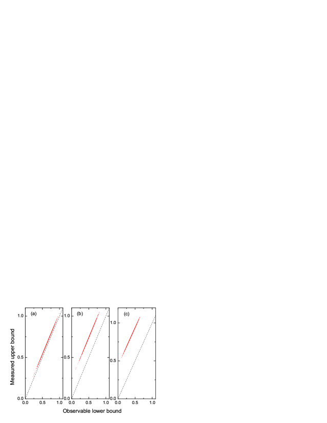
Figure 1: (Color online). Measurable upper bound $\mathrm{Tr}[\rho\otimes\rho(K_{1}+K_{2})/2]$ for squared mixed-state concurrence $[C(\rho)]^{2}$, versus its observable lower bound $\mathrm{Tr}[\rho\otimes\rho(V_{1}+V_{2})/2]$ for $3\times 3$-dimensional random states with different degrees of mixing: a shows weakly mixed states ($\mathrm{Tr}\rho^{2}=0.98$), b displays intermediate mixing ($\mathrm{Tr}\rho^{2}=0.88$), c corresponds to strongly mixed states ($\mathrm{Tr}\rho^{2}=0.78$). The dashed lines denote the lower bound.

Let us simulate the observable upper bound on mixed random states of $3\times 3$-dimensional systems. Mixed random states with different degrees of mixing were obtained via the generalized depolarizing channel channel , as Ref. Mintert3 did. The observable upper bound versus lower bound is shown in Fig. 1. Interestingly, the upper bounds in Fig. 1 are always in parallel with the lower bounds, which actually coincides with Eq. (7). For weakly mixed states, the bounds provide an excellent estimation of concurrence; for strongly mixed states, they also provide a region for concurrence.

Multipartite mixed states. The generalized concurrence for multipartite pure state is not unique. For instance, Ref. Mintert1 introduced several inequivalent alternatives. In this section, we choose the multipartite concurrence introduced in multi ; Mintert4 :

$$C_{N}(\Psi)\equiv 2^{1-N/2}\sqrt{(2^{N}-2)-\sum_{i}\mathrm{Tr}\rho_{i}^{2}},$$ (8)

where $i$ labels all $(2^{N}-2)$ different reduced density matrices. The definition can also be expressed as $C_{N}(\Psi)=\sqrt{\langle\Psi|\otimes\langle\Psi|A|\Psi\rangle\otimes|\Psi\rangle}$ with $A=4(\mathbf{P}_{+}-P_{+}^{(1)}\otimes\cdots\otimes P_{+}^{(N)})$. $\mathbf{P}_{+}$ ($\mathbf{P}_{-}$) is the projector onto the globally symmetric (antisymmetric) space Mintert4 . For mixed states, it is also given by the convex roof, $C_{N}(\rho)=\inf_{\{p_{i},|\Psi_{i}\rangle\}}\sum_{i}p_{i}C_{N}(\Psi_{i})$, for all possible decomposition into pure states, where $p_{i}\geq 0$ and $\sum_{i}p_{i}=1$. Ref. Mintert3 introduced lower bounds of squared concurrence for arbitrary multipartite states,

$$[C_{N}(\rho)]^{2}\geq\mathrm{Tr}(\rho\otimes\rho V),$$ (9)

with $V=4(\mathbf{P}_{+}-P_{+}^{(1)}\otimes\cdots\otimes P_{+}^{(N)}-(1-2^{1-N})\mathbf{P}_{-})$. We introduce an observable $K$ such that

$$[C_{N}(\rho)]^{2}\leq\mathrm{Tr}(\rho\otimes\rho K),$$ (10)

with $K=4(\mathbf{P}_{+}-P_{+}^{(1)}\otimes\cdots\otimes P_{+}^{(N)}+(1-2^{1-N})\mathbf{P}_{-})$. The proof of this inequality is shown in the following.

$$[C_{N}(\rho)]^{2} \leq \inf\sum_{i}p_{i}[C_{N}(\Psi_{i})]^{2}$$

$$= \inf\sum_{i}p_{i}2^{2-N}\sum_{k}c_{k}^{2}(\Psi_{i})$$

$$\leq 2^{2-N}\sum_{k}(2-\mathrm{Tr}\rho_{k}^{2}-\mathrm{Tr}\rho_{\overline{k}}^{2})$$

$$= 2^{2-N}\sum_{k}\mathrm{Tr}(\rho\otimes\rho\ 2(P_{-}^{(k)}\otimes\mathbbm{1}+\mathbbm{1}\otimes P_{-}^{(\overline{k})}))$$

$$= \mathrm{Tr}(\rho\otimes\rho K),$$

where $\sum_{k}$ is taken over all the bipartite concurrence $c_{k}$ corresponding to each subdivision of the entire system into two subsystems Mintert3 , $k$ denotes one subsystem and $\overline{k}$ denotes the other one. We have used that $\sum_{k}P_{-}^{(k)}\otimes P_{-}^{(\overline{k})}=2^{N-2}(\mathbf{P}_{+}-P_{+}^{(1)}\otimes\cdots\otimes P_{+}^{(N)})$ and $\sum_{k}(P_{-}^{(k)}\otimes P_{+}^{(\overline{k})}+P_{+}^{(k)}\otimes P_{-}^{(\overline{k})})=(2^{N-1}-1)\mathbf{P}_{-}$.

Inequality (10) also implies some interesting consequences: (1) The upper bound can also be expressed in terms of the purities of reduced density matrices, i.e., $\mathrm{Tr}(\rho\otimes\rho K)=2^{2-N}[(2^{N}-2)-\sum_{i}\mathrm{Tr}\rho_{i}^{2}]$, which coincides with Eq. (8) for pure state concurrence. (2) The upper bound can be directly measured, since it is given in terms of expectation values of symmetric and antisymmetric projectors. It is a little different from the lower bound $\mathrm{Tr}(\rho\otimes\rho V)$. (3) Interestingly, it is worth noting that

$$\mathrm{Tr}(\rho\otimes\rho K)-\mathrm{Tr}(\rho\otimes\rho V)=4(1-2^{1-N})(1-\mathrm{Tr}\rho^{2}),$$ (11)

i.e., the degree of mixing can be easily calculated out based on the upper and lower bounds.

We also simulate the observable upper bound on mixed random states of $2\times 2\times 2$-dimensional systems with different degrees of mixing obtained via the generalized depolarizing channel channel . The observable upper bound versus lower bound is shown in Fig. 2. The upper bounds in Fig. 2 are always in parallel with the lower bounds as well, which actually coincides with Eq. (11). For weakly mixed states, the bounds provide an excellent estimation of concurrence; for strongly mixed states, they also provide a region for concurrence.

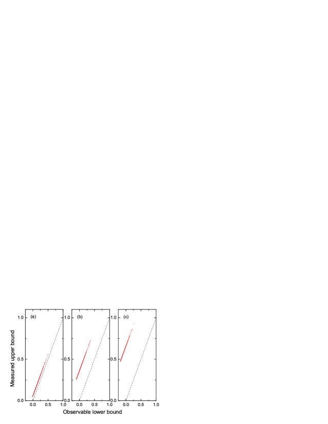
Figure 2: (Color online). Measurable upper bound $\mathrm{Tr}(\rho\otimes\rho K)$ versus its lower bound $\mathrm{Tr}(\rho\otimes\rho V)$ for $2\times 2\times 2$-dimensional mixed random states. Degrees of mixing are the same as Fig. 1.

III Relations with properties of the linear entropy

Interestingly, the upper and lower bounds of squared concurrence have certain relations with some properties of the linear entropy, such as the triangle inequality. The linear entropy is defined as follows linearentropy

$$E(\rho)\equiv 1-\mathrm{Tr}\ \rho^{2}.$$ (12)

It can be regarded as a kind of linearized von Neumann entropy $S(\rho)=-\mathrm{Tr}(\rho\log_{2}\rho)$, and has several same properties as $S(\rho)$. In the following, we will give simple proofs of the triangle inequality and subadditivity of the linear entropy.

The triangle inequality can be proved directly using the upper and lower bounds. Notice that the following inequalities hold for arbitrary bipartite states:

$$\begin{split}\mathrm{Tr}(\rho\otimes\rho K_{1})\geq[C(\rho)]^{2}\geq\mathrm{Tr}(\rho\otimes\rho V_{2}),\\ \mathrm{Tr}(\rho\otimes\rho K_{2})\geq[C(\rho)]^{2}\geq\mathrm{Tr}(\rho\otimes\rho V_{1}).\end{split}$$ (13)

Since Eqs. (5) and (6) hold, we can obtain some new inequalities,

$$\begin{split}1-\mathrm{Tr}\rho_{A}^{2}\geq\mathrm{Tr}\rho^{2}-\mathrm{Tr}\rho_{B}^{2},\\ 1-\mathrm{Tr}\rho_{B}^{2}\geq\mathrm{Tr}\rho^{2}-\mathrm{Tr}\rho_{A}^{2};\end{split}$$ (14)

$$\begin{split}1-\mathrm{Tr}\rho^{2}\geq(1-\mathrm{Tr}\rho_{B}^{2})-(1-\mathrm{Tr}\rho_{A}^{2}),\\ 1-\mathrm{Tr}\rho^{2}\geq(1-\mathrm{Tr}\rho_{A}^{2})-(1-\mathrm{Tr}\rho_{B}^{2}).\end{split}$$ (15)

Obviously, inequalities (15) can be directly calculated out from inequalities (14), and they are actually triangle inequalities of the linear entropy,

$$\begin{split}E(\rho_{AB})\geq E(\rho_{B})-E(\rho_{A}),\\ E(\rho_{AB})\geq E(\rho_{A})-E(\rho_{B}).\end{split}$$ (16)

Before embark on proving the subadditivity of the linear entropy, let us review the universal state inverter $\widetilde{\rho}$ introduced in Ref. rank2 ,

$$\widetilde{\rho} \equiv \mathrm{Tr}(\rho^{{\dagger}})\mathbbm{1}\otimes\mathbbm{1}-\rho_{A}^{{\dagger}}\otimes\mathbbm{1}-\mathbbm{1}\otimes\rho_{B}^{{\dagger}}+\rho^{{\dagger}}$$

$$= \sum_{\alpha}\sigma_{y}\otimes\sigma_{y}(Q_{\alpha}\rho Q_{\alpha})^{*}\sigma_{y}\otimes\sigma_{y},$$

where $Q_{\alpha}=P_{A}^{(ii^{\prime})}\otimes P_{B}^{(ii^{\prime})}$, $P_{A}^{(ii^{\prime})}=|i\rangle_{A}\langle i|+|i^{\prime}\rangle_{A}\langle i^{\prime}|$ and $P_{B}^{(jj^{\prime})}=|j\rangle_{B}\langle j|+|j^{\prime}\rangle_{B}\langle j^{\prime}|$. The universal state inverter $\widetilde{\rho}$ is a semi-positive definite operator, since each term in the sum $\sigma_{y}\otimes\sigma_{y}(Q_{\alpha}\rho Q_{\alpha})^{*}\sigma_{y}\otimes\sigma_{y}$ is semi-positive definite. Therefore, $\sqrt{\rho}\widetilde{\rho}\sqrt{\rho}$ has the semi-positive definite property as well, and we can obtain the following inequality,

$$1+\mathrm{Tr}\rho^{2}-\mathrm{Tr}\rho_{A}^{2}-\mathrm{Tr}\rho_{B}^{2}=\mathrm{Tr}\sqrt{\rho}\widetilde{\rho}\sqrt{\rho}\geq 0,$$ (17)

where we have used $\mathrm{Tr}\sqrt{\rho}\widetilde{\rho}\sqrt{\rho}=\mathrm{Tr}\rho\widetilde{\rho}=\mathrm{Tr}[\rho(\mathbbm{1}\otimes\mathbbm{1}-\rho_{A}\otimes\mathbbm{1}-\mathbbm{1}\otimes\rho_{B}+\rho)]=1+\mathrm{Tr}\rho^{2}-\mathrm{Tr}\rho_{A}^{2}-\mathrm{Tr}\rho_{B}^{2}$. Thus, $1+\mathrm{Tr}\rho^{2}-\mathrm{Tr}\rho_{A}^{2}-\mathrm{Tr}\rho_{B}^{2}\geq 0$ holds, i.e. the subadditivity of the linear entropy

$$E(\rho_{A})+E(\rho_{B})\geq E(\rho_{AB})$$ (18)

holds relation .

In fact, it is not the first time to prove the subadditivity of the linear entropy. For instance, Ref. Cai2 has proved the subadditivity of the linear entropy. Furthermore, the triangle inequality of the linear entropy can be proved from the subadditivity Preskill . Compared with this earlier proof, roughly speaking, our proof is a little simpler. The main purpose of this section is that these properties of the linear entropy are the natural results from the positive semidefiniteness of the universal state inverter and the upper and lower bounds, and they also indicate the validity of these bounds.

IV Discussions and conclusions

Actually, for two-qubit states, $\mathrm{Tr}(\rho\otimes\rho\cdot 4P_{-}^{(1)}\otimes P_{-}^{(2)})$ is a tighter upper bound of squared concurrence than $\mathrm{Tr}(\rho\otimes\rho K)$. Because the equation

$$\mathrm{Tr}(\rho\otimes\rho\cdot 4P_{-}^{(1)}\otimes P_{-}^{(2)})=\mathrm{Tr}\rho\widetilde{\rho}$$ (19)

holds for arbitrary two-qubit states, where $\widetilde{\rho}=\sigma_{y}\otimes\sigma_{y}\rho^{*}\sigma_{y}\otimes\sigma_{y}$. Eq. (19) has also been proved in Cai . Furthermore, notice that $C=max\{\lambda_{1}-\lambda_{2}-\lambda_{3}-\lambda_{4},0\}$, where $\lambda_{1},\lambda_{2},\lambda_{3},\lambda_{4}$ are squared roots of eigenvalues of $\rho\widetilde{\rho}$ in the decreasing order. Therefore, it is easily concluded that $\mathrm{Tr}(\rho\otimes\rho\cdot 4P_{-}^{(1)}\otimes P_{-}^{(2)})=\mathrm{Tr}\rho\widetilde{\rho}=\sum_{i}\lambda_{i}^{2}\geq(\lambda_{1}-\lambda_{2}-\lambda_{3}-\lambda_{4})^{2}\geq C^{2}$. However, the new upper bound $\mathrm{Tr}(\rho\otimes\rho\cdot 4P_{-}^{(1)}\otimes P_{-}^{(2)})$ is hard to generalize to arbitrary finite-dimensional bipartite states.

We give a brief discussion on the experimental measurement of our upper bound. As only the projector $P_{-}$ on one of the subsystems, rather than a complete set of observables, is required, our upper bound could be easily measured. In particular, for two-dimensional systems, $P_{-}$ is simply the projector onto the singlet state $|\Psi^{-}\rangle=(|01\rangle-|10\rangle)/\sqrt{2}$. Let us take the photonic system for example. The simplest way to project two photons onto the singlet state is using a Hong-Ou-Mandel interferometer PRL592044 . This method has been widely used since the teleportation nature390575 experiment. Another method, employed in nature ; nature2 , is distinguishing the Bell states with a controlled-NOT gate, which can transform the Bell states to separable states PRL744083 .

In conclusion, we present observable upper bounds of squared concurrence, which are the dual bound of the observable lower bounds introduced by Mintert et al.. These bounds can estimate entanglement for arbitrary finite-dimensional experimental unknown states by few experimental measurements on a twofold copy $\rho\otimes\rho$ of the mixed states. Furthermore, the degree of mixing for a mixed state and some properties of the linear entropy also have certain relations with its upper and lower bounds of squared concurrence. Last but not least, we discuss a tighter upper bound for two-qubit states only, and it remains an open question to generalize it to arbitrary finite-dimensional bipartite systems.

References

- (1) M. A. Nielsen and I. L. Chuang, Quantum Computation and Quantum Information (Cambridge University Press, Cambridge, 2000).
- (2) A. Einstein, B. Podolsky, and N. Rosen, Phys. Rev. 47, 777 (1935).
- (3) A. Osterloh, L. Amico, G. Falci, and R. Fazio, Nature (London) 416, 608 (2002).
- (4) R. F. Werner, Phys. Rev. A 40, 4277 (1989).
- (5) O. Rudolph, e-print arXiv:quant-ph/0202121; K. Chen and L.-A. Wu, Quantum Inf. Comput. 3, 193 (2003); H. Fan, e-print arXiv:quant-ph/0210168.
- (6) P. Aniello and C. Lupo, J. Phys. A: Math. Theor. 41, 355303 (2008); C. Lupo, P. Aniello, and A. Scardicchio, ibid. 41, 415301 (2008).
- (7) J.I. de Vicente, Quantum Inf. Comput. 7, 624 (2007); M. Li, S.-M. Fei, and Z.-X. Wang, J. Phys. A: Math. Theor. 41, 202002 (2008); O. Gühne, P. Hyllus, O. Gittsovich, and J. Eisert, Phys. Rev. Lett. 99, 130504 (2007).
- (8) J.I. de Vicente, J. Phys. A 41, 065309 (2008).
- (9) M. Seevinck and J. Uffink, Phys. Rev. A 76, 042105 (2007); J. Uffink and M. Seevinck, Phys. Lett. A 372, 1205 (2008).
- (10) D. Bruß, J. Math. Phys. 43, 4237 (2002); F. Mintert et al., Phys. Rep. 415, 207 (2005); M. B. Plenio, S. Virmani, Quantum Inf. Comput. 7, 1 (2007); R. Horodecki et al., e-print arXiv:quant-ph/0702225.
- (11) W. K. Wootters, Phys. Rev. Lett. 80, 2245 (1998); A. Uhlmann, Phys. Rev. A 62, 032307 (2000);
- (12) P. Rungta, V. Bužek, C. M. Caves, M. Hillery and G. J. Milburn, Phys. Rev. A 64, 042315 (2001).
- (13) H. Fan, K. Matsumoto and H. Imai, J. Phys. A 36, 4151 (2003); H. Fan, V. Korepin, and V. Roychowdhury, Phys. Rev. Lett. 93, 227203 (2004).
- (14) Y.-C. Ou and H. Fan, Phys. Rev. A 75, 062308 (2007); Y.-C. Ou, ibid., 75, 034305 (2007); H. Fan, Y.-C. Ou, and V. Roychowdhury, e-print arXiv:0707.1578; Y.-C. Ou, H. Fan, and S.-M. Fei, Phys. Rev. A 78, 012311 (2008).
- (15) K. Chen, S. Albeverio, and S.-M. Fei, Phys. Rev. Lett. 95, 210501 (2005); S.-M. Fei, Z.-X. Wang, and H. Zhao, Phys. Lett. A 329, 414 (2004).
- (16) A. Peres, Phys. Rev. Lett. 77, 1413 (1996); M. Horodecki, P. Horodecki, and R. Horodecki, Phys. Lett. A 223, 1 (1996); K. Życzkowski, P. Horodecki, A. Sanpera, and M. Lewenstein, Phys. Rev. A 58, 883, (1998); G. Vidal and R. F. Werner, Phys. Rev. A 65, 032314, (2002).
- (17) V. Coffman, J. Kundu, and W. K. Wootters, Phys. Rev. A 61, 052306 (2000); A. Wong and N. Christensen, ibid. 63, 044301 (2001); T. J. Osborne and F. Verstraete, Phys. Rev. Lett 96, 220503, (2006).
- (18) F. Mintert, M. Kuś and A. Buchleitner, Phys. Rev. Lett. 92, 167902 (2004); K. Chen, S. Albeverio and S.-M. Fei, Phys. Rev. Lett. 95, 040504 (2005); H. P. Breuer, J. Phys. A 39, 11847 (2006); J.I. de Vicente, Phys. Rev. A 75, 052320 (2007).
- (19) F. Mintert, M. Kuś, and A. Buchleitner, Phys. Rev. Lett. 95, 260502 (2005).
- (20) F. Mintert and A. Buchleitner, Phys. Rev. Lett. 98, 140505 (2007).
- (21) L. Aolita, A. Buchleitner, and F. Mintert, Phys. Rev. A 78, 022308 (2008).
- (22) L. Aolita and F. Mintert, Phys. Rev. Lett. 97, 050501 (2006).
- (23) F. Mintert, Appl. Phys. B 89, 493 (2007).
- (24) J. Eisert, F. Brandão, and K. Audenaert, New J. Phys. 9, 46 (2007).
- (25) O. Gühne, M. Reimpell, and R. F. Werner, Phys. Rev. Lett. 98, 110502 (2007); ibid., Phys. Rev. A 77, 052317 (2008).
- (26) C.-S. Yu and H.-S. Song, Phys. Rev. A 76, 022324 (2007); C.-S. Yu, C. Li, and H.-S. Song, ibid. 77, 012305 (2008).
- (27) X.-J. Ren, Z.-W. Zhou, X.-X. Zhou, and G.-C. Guo, Phys. Rev. A 77, 054302 (2008).
- (28) S. P. Walborn, P. H. Souto Ribeiro, L. Davidovich, F. Mintert, and A. Buchleitner, Nature 440, 1022 (2006);
- (29) S. P. Walborn, P. H. Souto Ribeiro, L. Davidovich, F. Mintert, and A. Buchleitner, Phys. Rev. A 75, 032338 (2007).
- (30) F.-W. Sun, J.-M. Cai, J.-S. Xu, G. Chen, B.-H. Liu, C.-F. Li, Z.-W. Zhou, and G.-C. Guo, Phys. Rev. A 76, 052303 (2007).
- (31) B. Terhal, Phys. Lett. A 271, 319 (2000); G. Tóth and O. Gühne, Phys. Rev. Lett. 94, 060501 (2005); F. A. Bovino, G. Castagnoli, A. Ekert, P. Horodecki, C. M. Alves and A. V. Sergienko, Phys. Rev. Lett. 95, 240407 (2005); O. Gühne and N. Lütkenhaus, ibid. 96, 170502 (2006); F. Mintert, Phys. Rev. A 75, 052302 (2007); R. Augusiak, M. Demianowicz, P. Horodecki, ibid. 77, 030301(R) (2008).
- (32) The first inequality has been proved in T. J. Osborne, Phys. Rev. A 72, 022309 (2005).
- (33) M. L. Aolita, I. García-Mata, and M. Saraceno, Phys. Rev. A 70, 062301 (2004).
- (34) A. R. R. Carvalho, F. Mintert, and A. Buchleitner, Phys. Rev. Lett. 93, 230501 (2004).
- (35) E. Santos and M. Ferrero, Phys. Rev. A 62, 024101 (2000).
- (36) Actually, it is also held that , since we have . Therefore, the proof of the subadditivity above has a little relations with the upper and lower bounds. Eq. (17) indicates that the average of the upper and lower bounds is nonnegative.
- (37) J.-M. Cai, Z.-W. Zhou, S. Zhang, and G.-C. Guo, Phys. Rev. A 75, 052324 (2007).
- (38) J. Preskill, Lecture Notes on Physics 229: Quantum Information and Computation, available at http://www.theory.caltech.edu/people/preskill/ph229/, Chapter 5, Exercise 5.2 (g). Although this exercise is for the von Neumann entropy, the same hint can be used for the linear entropy.
- (39) J.-M. Cai and W. Song, e-print arXiv:0804.2246.
- (40) C.-K. Hong, Z.-Y. Ou, and L. Mandel, Phys. Rev. Lett. 59, 2044 (1987).
- (41) D. Bouwmeester, J.-W. Pan, K. Mattle, M. Eibl, H. Weinfurter, and A. Zeilinger, Nature 390, 575 (1997).
- (42) A. Barenco, D. Deutsch, A. Ekert, and R. Jozsa, Phys. Rev. Lett. 74, 4083 (1995).