Kepler versus Akaike

Abstract

I use the example of the Earth’s orbit to illustrate the principle behind the Akaike Information Criterion, and refute the misconception that the criterion, by definition, discards more complex models in favour of simpler ones.

I Introduction

AIC Akaike is a model selection criterion, which takes into account how well a model explains the data, but also if the model is not too complicated. This is intuitively understood just by looking at the formula

$$\rm{AIC}=2k-2\ln L,$$ (1)

where $k$ is the number of parameters in the fitted model, and $L$ is the maximum value of the likelihood function. Thus, the better the fit, the lower the value of AIC. On the other hand, the number of the model’s parameters is considered to directly signify its complexity, increasing the value of AIC. The absolute value of AIC is not used, as it is the difference for a pair of models that matters: $\rm{AIC}_{1}-\rm{AIC}_{2}>0$ indicates that the second model is better than the first. The detailed mathematics of the criterion is not required here; a more complete introduction can be found for example in Burnham .

One may ask, if such a dependence on $k$ is not biased somehow – to promote models with as few parameters as possible or, perhaps, perfect agreement with the data points. This highly subjective question remains open, as there are many different information criteria on the market, and the concepts of simplicity of elegance of models have not to date been unanimously defined Dowe .

Nevertheless, it is possible to conduct an anachronic experiment – to test the test itself – by applying it to a solved problem in which a new, more complicated theory undoubtedly replaced the older one. In other words: if the past scientists had used model selection criteria, would physics have stopped at the stage of naive yet elegant theories, only to achieve simplicity instead of agreement with experiment?

The idea of applying AIC to a classical problem (the shape of the Earth’s orbit in this case) was born when a referee of Szydlowski gave what he thought was a counterexample to applicability of such a criterion. It turns out that the calculations show exactly the opposite.

II The “experiment”

The difference between an ellipse and a circle is a clear example of the complexity-accuracy trade-off. Is it really necessary to include two new parameters: the eccentricity and the anomaly of the perihelion? Why not stick to a simple circular orbit which is roughly the same?

Imagine we measure the distance to the Sun daily. If one is interested in its relative value it suffices to measure the position $\varphi$ of the Sun, which translates into angular velocity $\varphi^{\prime}(t)$. Assuming next that the field velocity is constant, one readily obtains the relative distance

$$\frac{r_{i}}{r_{j}}=\sqrt{\frac{\varphi^{\prime}(t_{j})}{\varphi^{\prime}(t_{i})}}.$$

Of course, this is partially a thought experiment, so that we have to ignore some practical questions like how exactly the angles are to be measured. On the other hand, we obviously assume radar has not yet been invented and only allow for astrometric means.

Say we perform 50 observations a day for the whole year, averaging so that there are 365 data points consisting of pairs $(\varphi_{i},r_{i})$. If the orbit is elliptic then the change of $\varphi$ will vary with each day. To remedy this one could say that the observing takes places at different times and since the angle is also measured the data is accordingly reduced. Also, the differences will not be big for our orbit, and it is necessary to estimate the total errors arbitrarily anyway – this is a thought experiment after all. Accordingly, the anomaly $\varphi$ will be taken as known exactly and distributed evenly between $0$ and $2\pi$.

The above setup allows us to use the simple orbit equation for the radius

$$r=\frac{p}{1+e\cos(\varphi-\varphi_{0})},$$ (2)

where $e$ is the eccentricity, $\phi_{0}$, is the perihelion anomaly, and $p$ is the distance at $\varphi=\varphi_{0}+\pi/2$. For a circle $e=0$, so there are $k_{1}=0$ parameters. The other orbit requires $k_{2}=2$ parameters. How does one choose the day to use the corresponding radius as reference, and get rid of $p$? Since $\varphi_{0}$ is unknown, we could for example take the mean reciprocal radius

$$\langle r^{-1}\rangle=p^{-1}\langle 1+e\cos(\varphi-\varphi_{0})\rangle=p^{-1}.$$

The left hand side is obtained from the observations, and the right hand side is an integral over $d\varphi$ – a justified approximation taking into account the number of the data points, and the hypothetical nature of the experiment.

Obviously, the data has to be simulated, to be as expected for an elliptic orbit with Gaussian errors $\epsilon(0,\sigma)$ of mean $0$ and standard deviation of $\sigma=0.5$ for a single observation. Note that the distance is relative, so the error corresponds to uncertainty of half of the orbits (mean) radius. That is quite a lot but we are also simulating the limitations of “ancient” astronomy.

To be more concrete, I took 365 values of the anomaly $\varphi_{i}=(i-1)/365$, $i=1,\ldots,365$, and for each $i$, corresponding $50$ values of the radius

$$r_{i,l}=\frac{1}{1+0.0167\cos[2\pi\frac{i-1}{365}]}+\epsilon_{i,l}(0,\sigma),\;\;l=1,\ldots,50,$$ (3)

where the numerical value of eccentricity was used, and $i=1$ coincides with the minimal radius. Which is not to say, the hypothetical observer knows this fact. A value of the perihelion anomaly will also have to be found when fitting.

Next, I calculated, for each value of $\varphi_{i}$, the mean $r_{i}$, and its error

$$r_{i} =\frac{1}{50}\sum_{l=1}^{50}r_{i,l},$$

$$\sigma_{i} =\sqrt{\frac{1}{50}\frac{1}{49}\sum_{l=1}^{50}(r_{i,l}-r_{i})^{2}}.$$

And the respective likelihoods are

$$L_{1}=\exp\left[-\frac{1}{2}\sum_{i=1}^{365}\left(\frac{1-r_{i}}{\sigma_{i}}\right)^{2}\right],$$ (4)

$$L_{2}=\exp\left[-\frac{1}{2}\sum_{i=1}^{365}\left(\frac{\frac{1}{1+e\cos(\varphi_{i}-\varphi_{0})}-r_{i}}{\sigma_{i}}\right)^{2}\right],$$ (5)

where a multiplicative constant was omitted for brevity.

Maximising the above, one obtains the values of $L_{1}$ and $L_{2}$ required for formula (1) (and, of course $\varphi_{0}$ and $e$ but these are unimportant for this experiment). To make sure the result is not just a coincidence I calculated the mean $\Delta\rm{AIC}=\rm{AIC}_{1}-\rm{AIC}_{2}$ and its error for $100$ such observational setups to get

$$\Delta\rm{AIC}=8.16\pm 0.76.$$ (6)

III Conclusions

Figures 1 and 2 show typical data points (black), together with the fitted elliptic orbit (blue) and circular orbit (red). AIC gives clear indication in favour of the ellipse even for such high level of noise. Thus, at least at this point, the progress of physics would not have been inhibited by model comparing criteria, and the seemingly more complicated theory would have been chosen. The numbers and figures speak for themselves, but it is also worth mentioning that if the errors are reduced only to $0.1$ the mean $\Delta$AIC increases drastically to the value of $263.3\pm 3.3$. On the other hand, when $\sigma$ is put equal $0.9$, the evidence is $\Delta$AIC $=0.73\pm 0.53$, which cannot be called conclusive, but is still positive despite the unrealistic error of 90% the radius length.

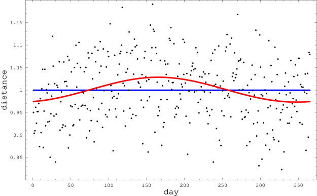
Figure 1: Radius plotted against the day number for the simulated data points (black), the fitted elliptic curve (blue) and the circular orbit (red).

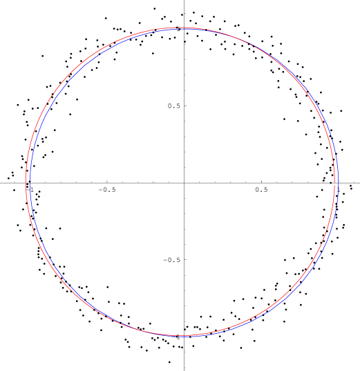
Figure 2: Polar plot of the simulated data points (black), fitted elliptic orbit (blue) and circular orbit of radius $1$ (red).

Hopefully, this example will help to understand that model selection criteria take into account not only the number of parameters but also the agreement with the data. This is not to say that AIC is the criterion of simplicity or elegance of models, but that it still gives a reasonable estimate of complexity (parameters) versus applicability (fitting) of models.

References

- (1) H. Akaike, “A new look at the statistical model identification,” IEEE Transactions on Automatic Control 19, (6): 716-723, (1974)
- (2) K. P. Burnham and D. Anderson “Model Selection and Multi-Model Inference,” Springer Verlag, New York.
- (3) D. L. Dowe, S. Gardner and G. Oppy, “Bayes not Bust! Why simplicity is no problem for Bayesians,” British Journ. Phil. Sci. 58, (4): 709-754, (2007)
- (4) M. Szydlowski and W. Godlowski, “Can brane dark energy model be probed observationally by distant supernovae?” Phys. Lett. B639, 5-13, (2006)