Gravitational clustering: an overview

Abstract

We discuss the differences and analogies of gravitational clustering in finite and infinite systems. The process of collective, or violent, relaxation leading to the formation of quasi-stationary states is one of the distinguished features in the dynamics of self-gravitating systems. This occurs, in different conditions, both in a finite than in an infinite system, the latter embedded in a static or in an expanding background. We then discuss, by considering some simple and paradigmatic examples, the problems related to the definition of a mean-field approach to gravitational clustering, focusing on role of discrete fluctuations. The effect of these fluctuations is a basic issue to be clarified to establish the range of scales and times in which a collision-less approximation may describe the evolution of a self-gravitating system and for the theoretical modeling of the non-linear phase.

1 Introduction

As discussed in various papers in this volume (see e.g.intro ; campa ) equilibrium properties of long-range interacting systems require a non-trivial analysis as standard thermodynamics techniques do not simply apply when dealing with pair-interactions decaying with sufficiently small exponents. Many interesting and unsolved problems lie in the out-of-equilibrium dynamics of systems with long-range interaction about which very little is known from a theoretical point of view (see also chavanis in this volume). The understanding of the thermodynamics and dynamics of systems of particles interacting only through their mutual Newtonian self-gravity is of fundamental importance in cosmology and astrophysics. It encompasses the range of physical scales relevant to the formation of the largest structures in the Universe, down to those relevant to stellar dynamics. The statistical mechanics of systems dominated by gravity has been studied and applied in many different contexts in astrophysics and cosmology (see e.g. lyndebell ; pad_physrep ; chavanis ; chandra ; chandra_revmodphy ; pad_book ; pad_dtslri ; saslaw1 ; saslaw2 ; binney ; peebles ; thierry ): for example in the studies of globular clusters, galaxies and the clustering in the expanding universe.

While systems with short range interactions can be usually studied through laboratory experiments, gravitational systems can only be observed in astrophysical contexts. Alternatively one may set up numerical experiments which then represent the unique instrument to study the dynamics of gravitational clustering. In this respect the astrophysicist’s perspective is usually to model some intricate realistic systems, such as stellar or galaxy systems, having the aim of understanding a specific set of observations. For example in the cosmological context one uses very complicated initial conditions (described by a large number of parameters) and needs a certain number of important assumptions, from the way the universe expands to the amount and type of dark matter which dominates the dynamics on the relevant scales. This is so because, by studying gravitational clustering, one would like to understand the relations between some important observations of the cosmos. For example the studies of the cosmic microwave background radiations provide with the information about the initial conditions of the matter density field. The large scale geometrical properties of the universe are deduced, for example, through the measurements of the supernovae magnitude-redshift relation. Galaxy redshift surveys map the present-day matter distribution. The estimations of the mass-to-light ratio of astrophysical objects is ultimately related to the abundance of dark matter. The task of the model of cosmological structure formation is thus to build a unified and coherent picture to explain these (and other) observations of the universe at the largest scales peacock .

In statistical physics the problem of the evolution of self-gravitating classical bodies has been relatively neglected, primarily because of the intrinsic difficulties associated with the attractive long-range nature of gravity and its singular behavior at vanishing separation. When approaching the problem of gravitational clustering in the context of statistical mechanics it is natural to start by reducing as much as possible the complexity of the analogous cosmological or astrophysical problem. For example, in order to focus on the essential aspects of the problem one may study gravitational clustering without the expansion of the universe, and starting from particularly simple initial conditions. With respect to the motivation from cosmology/astrophysics, there is of course a risk: in simplifying we may loose some essential elements which change the nature of gravitational clustering. Even it were, it seems unlikely that we will not learn something about the more complex cosmological/astrophysical situations in addressing slightly different and simplified problems.

A fundamental distinction has to be made between finite and infinite systems. They have in common that the gravitational force on a arbitrary point has contributions coming from all scales in the system. However they differ for the fact that in the case of the finite system there is a mean field force generated by the system as a whole, which is related to its internal symmetries (e.g., spherical symmetry) and which eventually will give rise to a global collapse of the entire system. In an infinite space, in which the initial fluctuations are non-zero and finite at all scales, the collapse of larger and larger scales will continue ad infinitum: being no geometric center there will not be a global collapse of the entire system. The mean field dynamics is driven by system’s fluctuations which determine the gravitational force at different spatial scales. The collapse occurring on larger and larger scales will clearly happen at different times but it is characterized by the unique time-scale in the system that is

$$\tau\sim\sqrt{G\rho_{0}}^{-1}\,.$$ (1)

This is in general the typical characteristic time scale of any (finite or infinite) gravitational system with average mass density $\rho_{0}$. For instance, as we discuss below, this is the time scale predicted by the self-gravitating fluid approximation.

The infinite system can therefore never reach a time independent state, and in particular it will never reach a thermodynamic equilibrium. Although so different, the finite and the infinite systems share some subtle and important analogies which we briefly discuss in what follows. We firstly discuss the general difficulties related to the long-range character of gravity and the usual way to make a mean-field approximation. Then we consider two basic examples of a finite and of an infinite system: the simplest example of a finite system is represented by an initially isolated spherical distribution of randomly distributed points (i.e. a Poisson distribution) — this will be also discussed in the contribution by Morikawa in this book morikawa . Analogously the simplest example of an infinite system is a Poisson distribution in an infinite space. For this second case one may consider that the space background is static (as Joyce in his contribution in this book joyce ) or it is expanding (as Saslaw in his contribution saslaw ). We will discuss these two cases briefly, outlining the analogies and the differences. In the conclusions we try to point out which are the main problems of the field.

2 Gravitational relaxation and mean field models

The typical feature of short-range interactions system is that the force between two particles (e.g. molecules of an ordinary gas) is strong when they are very close to each other, i.e. when they repeal each other strongly, and on large distances no force is exerted between two particles. In this way particles most of time move at nearly constant velocity, and then they are subject to violent and short lived accelerations when they collide with one another. In this situation, the typical mechanism for relaxation is that due to two-body collisions. For self-gravitating particles the situation is different because gravity is divergent at vanishing separation and it is long range. Because of the former property the actual force on a given particle maybe more or less strongly influenced by fluctuations in its local neighborhood, while the latter property implies that a particle is coupled with all other particles at all scales in the system. Thus the studies of a self-gravitating systems have to consider that many different range of scales, in principle all, maybe almost equally important for the analysis of the dynamical properties.

For this reason, one the principal problems of stellar dynamics chandra ; chandra_revmodphy is concerned with the analysis of the nature of the gravitational force acting, for example, on a star which is member of a stellar system. In a general way we may broadly distinguish between the influence of the system as a whole $\vec{F}_{sm}$ and of the immediate neighborhoods $\vec{F}_{f}$. The former will be smoothly varying function of position and time while the latter will be subject to relatively rapid fluctuations:

$$\vec{F}=\vec{F}_{sm}+\vec{F}_{f}\;.$$

The second term describes the fluctuations that are related to the underlying statistical properties of the particle distribution: their effects can be evaluated, under certain assumptions, in a stochastic sense.

The problem is general is to establish a criterion to quantitatively determine the circumstances under which

$$\vec{F}\approx\vec{F}_{sm}\;,$$ (2)

and thus $\vec{F}_{f}\approx 0$, i.e. under which the system can be treated by the mean field approximation. This consists in neglecting the local interaction and to consider the global gravitational field of the system. This is not an easy task for the general case. For example in the simplest situation of an isolated self-gravitating system in virial equilibrium it is possible to estimate a criterion for using the approximation provided with Eq.2, by considering the role of two-body scattering chandra ; binney ; saslaw2 . Whether this can be used for the more general case of an out-of-equilibrium system is an open question binneyknebe ; diemond ; power02 .

As mentioned above, the mean field approximation consists in neglecting the physics on small scales in the system and for this reason it usually describes a collision-less system. We briefly recall the main steps to obtain such an approximation binney ; pad_physrep ; saslaw2 . Let us divide the phase space of a given system into a large number of cells in such a way that (i) each cell is large enough to contain a macroscopic number of particles (ii) each cell is small enough so that all particles in the cell can be assumed to have the same average characteristic properties of the cell. Thus the size of the cell should be large enough to satisfy (i) but not so large to violate (ii). If such an intermediate size can be defined at a generic time $t$ it is possible to define smooth functions, as for example the one-point distribution function. As the collapse will involve progressively larger and larger scales this approximation may break down at a certain time, when non-linear objects will be formed on the scale of the cell.

In the approximations above discussed the one-point distribution function will satisfy the Boltzmann equation. By neglecting the collision terms one may obtain the collision-less Boltzmann equation or Vlasov equation which is the basic tool to study the evolution of self-gravitating systems. From the Vlasov-Poisson system of equations one may derive, by considering other suitable approximations, the equations describing the evolution of a self-gravitating fluid. In this treatment the discrete nature of a particle distribution is neglected in the dynamical evolution: we will come back on this point below.

3 Finite systems

We now consider a very simple model to describe the dynamics of an isolated finite system. Let us suppose to have an initial uniform distribution of $N$ points of identical mass $m$ in a spherical volume of radius $R_{0}$ and density

$$\rho_{0}=Nm\frac{3}{4\pi R_{0}^{3}}\;.$$

We suppose that this system is isolated in an infinite space. Let us consider the limit of a perfect uniform system

$$\lim_{N\rightarrow\infty,\;\;m\rightarrow 0}Nm=\mbox{const}\;,$$

where the fluctuations in the system also go to zero in the same limit. The mass contained in a sphere of radius $r_{0}\leq R_{0}$ is just

$$M(r_{0})=\int_{0}^{r_{0}}4\pi r^{2}\rho_{0}dr=\frac{4\pi}{3}r_{0}^{3}\rho_{0}\;.$$ (3)

For reasons of spherical symmetry, the force exerted on a particle of unitary mass in the point at distance $r_{0}$ from the center of the sphere is due to the matter inside the shell

$$F(r_{0})=-\frac{GM(r_{0})}{r_{0}^{2}}\;.$$ (4)

This force is radial and directed toward the center of the sphere. For simplicity we suppose that the initial velocities are zero so that the initial total energy is equal to the initial potential energy and thus it is negative. In addition, we make the assumption that different shells do not overlap during the collapse. Thus the point initially at $r_{0}$ will be attracted by the same mass $M(r_{0})$ at all times but with varying force. The equation of motion can be written as

$$\ddot{r}(t)=-\frac{GM(r_{0})}{r^{2}(t)}\;.$$ (5)

This can be integrated to give

$$\left(\frac{dr}{dt}\right)^{2}=2GM(r_{0})\left(\frac{1}{r}-\frac{1}{r_{0}}\right)\;,$$ (6)

where $G$ is the Newton’s constant. The solution of this equation can be written in a parametric form

$$r(\xi)=\frac{r_{0}}{2}(1+\cos(\xi))$$ (7)

$$t(\xi)=\sqrt{\frac{3}{32\pi G\rho_{0}}}\left(\xi+\sin(\xi)\right)\;,$$

where

$$r(\xi=0)=r_{0}\;\;\;\mbox{at}\;\;\;t(\xi=0)=0$$ (8)

$$r(\xi=\pi)=0\;\;\;\mbox{at}\;\;t(\xi=\pi)=\sqrt{\frac{3\pi}{32G\rho_{0}}}\equiv\tau_{scm}\;.$$

Thus this evolution describes the collapse from the time $t=0$ at which the system has radius $R_{0}$ to the time $\tau_{scm}$ at which the system has zero radius. At longer times the system will re-expand up to reach the initial configurations, and then will continue these oscillations periodically. It is interesting to note that in this model the system never reaches a virialized state (although the total energy is negative).

There are some essential aspects of the problem which this approach is missing. It is in fact well known through the studies of computer experiments, that a system of particles is well described by Eq.3 at times prior to $\tau_{scm}$, while it differs for $t\rightarrow\tau_{scm}$, when the particle system goes through a phase of collective relaxation which brings a part of particles to form a quasi-equilibrium configuration in virial equilibrium. Total collapse will never occur because small initial inhomogeneities in the system, always present in any particle distribution, will generate random motions which will eventually stop the collapse (see Fig.1).

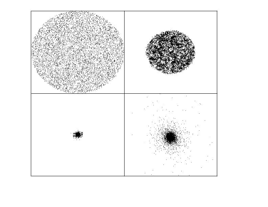
Figure 1: Different phases of the spherical cold collapse (projection of the $x-y$ plane of a thin slice around the center of the system, chosen, at different times, to have the approximately the same number of points inside): top-left initial distribution, top-right at $t=0.8\tau_{scm}$, bottom-left at $t=1\tau_{scm}$ and bottom-right at $t=2\tau_{scm}$. From this latter time on the structure is virialized and a forms quasi-stationary state.

In this situation the system forms a state characterized by a dense central region in virial equilibrium surrounded by a low-density halo made of particles with positive total energy. The subsequent evolution is driven by collisions: particles in the high density central region can undergo to two-body scatterings. The integrated effect of these collisions is that a part of the particles gain some kinetic energy while the others end up in a more bounded state. The long term consequence of these close encounters is the so-called evaporation, i.e. that the core becomes more and more bounded and looses little by little its particles by ejecting them. Thus the asymptotic state should be made of very few (in principle two) particles orbiting one around the others, very close so to keep all the potential energy of the system, and an ideal gas made by the other particles which can move freely bringing the main part of the kinetic energy of the system (see Fig.2).

Lynden-Bell lyndebell , who named the collective relaxation process as “violent relaxation”, made the first attempt to construct a theory describing the process of gravitational collapse by considering a collision-less system. While the process of violent relaxation is the main mechanism for relaxation of self-gravitating systems, in very different situations, it is still not completely understood in its full details and the theory of Lynden-Bell has shown various disagreements when compared with the results with N-body simulations even for the simplest case illustrated above (the same occurs with other theoretical attempts — see e.g. violrelax ).

The violent relaxation process acts on a time scale $\tau_{scm}$ which is much shorter than, for example, the typical time scale for two-body collisions $\tau_{2}$, which sets the time scale for the evaporation of the core-halo structure mentioned above. Indeed one may show saslaw2 ; binney that for a system of $N$ particles this goes as

$$\tau_{2}\propto\frac{N}{\log(N)}\tau_{scm}\;.$$

This situation outlines an important difference between systems with long and short range interactions. As mentioned, for systems with short-range forces the relaxation proceeds through collisions. Self-gravitating systems instead relax through processes other than the collisional relaxation, such as violent relaxation, which operate on time scales which are much shorter than the two-body relaxation time. In fact, the collisional relaxation time for several astrophysical systems is larger than the age of the universe and for many years this was considered a paradox (see e.g. saslaw2 ): how can globular cluster be in virial equilibrium if their relaxation time (supposed to be given by $\tau_{2}$) is longer than the age of the universe ? The answer was simply that the relaxation mechanism was different from two-body collisions.

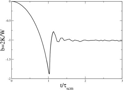
Figure 2: Virial ratio $b=2K/W$, where $K$ is the total kinetic energy of the bound particles and $W$ their gravitational potential energy, as a function of time: At times $t>\tau_{scm}$ we have that $b\approx-1$ and hence the virial theorem is satisfied.

Thus the complete theoretical characterization of the simple spherical collapse of cold particles described above, is an important and still open problem not only for astrophysics but also for cosmology. Indeed in both contexts one observes, in numerical simulations, the formations of core-halo structures (we will come back below on the cosmological simulations and on the structures formed therein). Thus a mechanism similar to the violent relaxation of a finite system is essential also for the virialization of larger and larger clusters of particles in an infinite system although with some important differences white ; morikawa . As in the finite system, also in the infinite system the two-body relaxation time scale is much longer than the real relaxation time of structures. Because the mean field force is due to fluctuations, the time-scales for the collapse of an over-density of given size is much longer in the infinite system than in the finite system case.

The ultimate task of a theory describing the process of violent relaxation should be the prediction of the quasi-stationary (virialized) state, which can be generally described by the Vlasov equation, given the initial conditions in terms of the phase space density (see e.g. hansen ). In particular there is a full set of properties of the virialized state, such as the density profile, the velocity distribution and profile, and their relations, which seems to be universal, i.e. appearing from many different initial conditions (see e.g. morikawa ) and that are currently unexplained from a theoretical point of view.

Finally we note that being the two-body relaxation time larger than $\tau_{scm}$ when the number of particles is large enough, the collisional effects can usually be neglected for self-gravitating quasi-equilibrium virial states, which can be treated with an appropriate non-collisional (i.e. Vlasov) approximation. However in general the problem consists in the comprehension of the role of collisions and of the terms related to discreteness (i.e. random forces, etc.) during the out-of-equilibrium phase, i.e. during collapse giving rise to a stationary configuration. We will come back to this point in what follows.

4 Infinite systems

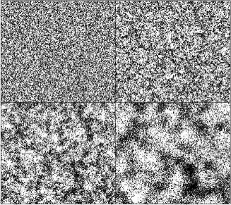
Figure 3: Evolution of the fluctuations and formation of structures in a simulation (with periodic boundary conditions, representing the infinite system case) started from cold Poisson initial conditions. Structures form firstly on small scales (top-left and top-right) and then propagate to larger and large scales (bottom-left and bottom-right).

The problem of the evolution of self-gravitating classical bodies, initially distributed very uniformly in infinite space, is as old as Newton. Modern cosmology poses essentially the same problem as the matter in the universe is now believed to consist predominantly of almost purely self-gravitating particles — so called dark matter — which is, at early times, indeed very close to uniformly distributed in the universe, and at densities at which quantum effects are completely negligible. Despite the age of the problem and the impressive advances of modern cosmology in recent years, our understanding of it remains, however, very incomplete. In its essentials it is a simple well posed problem of classical statistical mechanics.

The standard paradigm for formation of large scale structure in the universe is based on the growth of small initial density fluctuations in a homogeneous and isotropic medium. In the currently most popular cosmological models, a dominant fraction (more than 80 %) of the clustering matter in the universe is assumed to be in the form of microscopic particles which interact essentially only by their self-gravity. At the macroscopic scales of interest in cosmology the evolution of the distribution of this matter is then very well described by the Vlasov equation coupled with the Poisson equation binney ; pad_physrep ; saslaw1 ; saslaw2 .

A full solution, either analytical or numerical, of these equations starting from appropriate initial conditions is not feasible. In cosmology perturbative approaches to the problem, which treat the very limited range of low to modest amplitude deviations from uniformity, have been developed but numerical simulations are essentially the only instrument beyond this regime and to study the non-linear phase . N-body simulations solve numerically for the evolution of a system of $N$ particles interacting purely through gravity, with a softening at very small scales. The number of particles $N$ in the very largest current simulations is $\sim 10^{10}$ millenium , many more than two decades ago, but still many orders of magnitude fewer than the number of real dark matter particles ($\sim 10^{80}$ in a comparable volume for a typical candidate). While such simulations constitute a very powerful and essential tool, they lack the valuable guidance which a fuller analytic understanding of the problem would provide. The question inevitably arises of the accuracy with which these “macro-particles” trace the desired correlation properties of the theoretical models. This is the problem of discreteness in cosmological N-body simulations. It is an issue which is of considerable importance as cosmology requires ever more precise predictions for its models for comparison with observations.

As already mentioned, the infinite system can never reach a time independent state (see Fig.3). However one of the important results from numerical simulations of such systems in the context of cosmology is that the system nevertheless reaches a kind of scaling regime, in which the temporal evolution is equivalent to a rescaling of the spatial variables efts88 ; smith2003 . This spatio-temporal scaling relation is referred to as “self-similarity” and this behavior is usually observed for the time evolution of the two-point correlation function or its Fourier transform, the power spectrum (see Fig.4). Before describing this evolution in more detail let us come back to the determination of the gravitational force on an average particle in a certain distribution and to the approximations usually employed to study clustering in an infinite system.

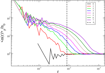
Figure 4: Evolution of the two-point correlation function in a Poisson simulation with periodic boundary conditions (representing an infinite system). The temporal evolution of this statistical quantity is equivalent to a rescaling of the spatial variables. The time indicated in the labels is given in units of the dynamical time scale $\tau=\sqrt{4\pi G\rho_{0}}^{-1}$ of the system. The distance scale $\Lambda_{i}$ marks the initial average distance between nearest particles.

4.1 The force distribution

Let us consider a uniform particle distribution book in a finite volume $V$. The actual value of the gravitational force per unit mass acting on a fixed “test” particle belonging to the system, supposed to be on the point $\vec{x}$ due to all the other $N$ system particles is given by

$$\vec{F}(\vec{x})=-Gm\sum_{i=1}^{N}\frac{\vec{x}-\vec{x}_{i}}{|\vec{x}-\vec{x}_{i}|^{3}}$$ (9)

where $m$ is the particle’s mass, supposed to be the same for all particles, and $\vec{x}_{i}$ the position vector of the $i^{th}$ particle. The sum in Eq.9 is extended to all the particles other than the test one, which are contained in the system volume $V$ Eventually $V\rightarrow\infty$ and $N\rightarrow\infty$ in such a way that the average number density $n_{0}=N/V$ remains constant. The actual value of $\vec{F}$ clearly depends on the nature of the local particle distribution, and hence, it will be in general subjected to stochastic fluctuations. These fluctuations determine a more or less broad force probability density function (PDF) $P(\vec{F})$. Because of statistical isotropy the direction of $\vec{F}$ is completely random with equal probability in each direction, i.e. $P(\vec{F})$ depends only on $F=|\vec{F}|$. Thus one may simply consider $P(\vec{F})d\vec{F}=4\pi F^{2}W(F)dF$, where $W(F)$ is the PDF of the modulus of the force. For reasons of spherical symmetry the average gravitational force acting on one system’s particle and due to the rest of the system vanishes. Any force acting on a particle is due to fluctuations away from exact (i.e. deterministic) spherical symmetry.

Chandrasekhar chandra_revmodphy (see also book ; force ) has considered the behavior of the PDF of the Newtonian gravitational force arising from a statistically isotropic (infinite) Poisson distribution of sources. He showed that applying the Markov method, it is possible to compute exactly the PDF, known as the Holtzmark distribution, of the gravitational force acting on a test particle in the system.

A very simple and approximate way to compute this PDF is to consider only the contribution of the first neighbor: in this way from the nearest neighbor (NN) probability distribution one may get the PDF of the force. An interesting point is that the Holtzmark distribution and the approximated PDF derived by considering the contribution of only the NN agree very well in the large $F$ region (see Fig.5).

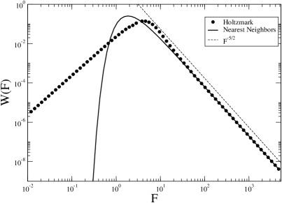
Figure 5: Holtzmark distribution and the PDF inferred if only NNs contribute, i.e., $W_{NN}(F)dF=\omega(r)dr$ being $\omega(r)$ the NN PDF. The agreement is very good in the strong field limit where $W(F)\sim F^{-5/2}$. At weak field the PDF due to the NN has a sharp cut-off while the full Holtzmark distribution shows a more gentle decrease (see discussion in book ; force ; earlytimes ).

The region where they differ most is when $F\rightarrow 0$. This is due to the fact that a weak force can arise only from a more or less symmetric configuration of particles around the test one in which fluctuations are determined by many particle effects, and hence the NN approximation fails. Instead in the strong field limit we may almost neglect the contribution to the force from far away points, because the main contribution is due to the limit $r\rightarrow 0$ in the elementary interaction (i.e. it comes from the NN). Note that, as in the NN case, because of the behavior of $W(F)$ for $F\rightarrow\infty$, $\langle F^{2}\rangle$ diverges. This is due to the singularity of the particle-particle gravitational interaction $\sim 1/r^{2}$ at $r=0$ together with the fact that in the Poisson distribution there is no explicit positive minimal distance between particles (i.e. no lower cut-off), as they are permitted to be at an arbitrarily small distance from one another.

The extension of the Holtzmark distribution to other statistically homogeneous and isotropic distributions is in general not straightforward, the main complication being introduced by the presence of spatial correlations among particles. One may find in book ; force ; masucci ; pellegrini (and references therein) the derivation of the PDF, under certain assumptions, for particle distributions with non-trivial correlations.

4.2 The infinite static case

In the previous derivation we used an important assumption (see also joyce in this volume), which we now examine in more detail. The sum defined in Eq.9 is not well defined because it is only conditionally convergent for $V\rightarrow\infty$, i.e. its result depends on the order in which the single terms are summed. Thus the assumption is that the sum has been taken symmetrically with respect to the point $\vec{x}$. Other prescriptions will in general lead to different results. To see more clearly this fact let us consider the local particle density embedded in a uniform background of negative mass density so that the microscopic mass density is

$$\delta\rho(\vec{x})=m(n(\vec{x})-n_{0})$$ (10)

where $n(\vec{x})$ is the local particle density with average density $n_{0}$ and the second term represents the uniform background. In this situation the force on a particle is a well defined stochastic quantity, i.e. it does not depend on how the volume $V$ is sent to infinity force . Given that the limit $V\rightarrow\infty$ does not depend on the way the limit is performed, one can choose for simplicity to take the volume $V$ symmetric with respect to the point $\vec{x}$ where the force is computed. In such a volume the contribution to the force from the uniform background vanishes by symmetry and thus, with this choice of the volume $V$, the force coincides with the limit of the sum in Eq.9.

While it is possible to show that the presence of an analogous background with negative mass density comes naturally when the motion of a particle is described in comoving coordinates in an expanding universe, in pure Newtonian gravity such a background does not exist and has to be introduced artificially to regularize the problem (Jean’s swindle). The negative mass density background is equivalent to the condition that the force is summed symmetrically (see also force ; joyce ). Note that this modification does not necessarily make the gravitational force well defined in general: whether it is well defined depends on the nature of the correlations between fluctuations in the density field on large scales (see discussion in force ) .

Let us now consider the evolution from an initially cold (i.e. zero velocity) Poisson distribution. Given that the PDF of the gravitational force is well approximated by the NN one for large fields, we can make a simple test: run a gravitational N-body simulation starting from a cold Poisson distribution (nominally infinite), with only this component of the force and then compare it with the situation occurring in the case the full gravity force is considered bsl04 . The approximate NN simulation is able to reproduce the formation of the first structures, made by clusters of two particles, up to the typical time scale $\tau_{NN}$ for two particles initially placed at a distance $\ell$, the initial average distance between NN, to collapse on each other. This is (again) of the order of

$$\tau_{NN}\sim\sqrt{Gm/\ell^{3}}^{-1}\sim\sqrt{G\rho_{0}}^{-1}\;,$$ (11)

where $\rho_{0}=mn_{0}$ and $n_{0}\sim\ell^{-3}$ is the number density. In particular it is very interesting to note that the form of the two-point correlation function in the non-linear regime, which as already mentioned will be preserved during time evolution because of its “self-similar” behavior, forms during this NN phase. This is not all however as the NN truncation will loose an important aspect of the gravitational evolution, that on large scales, i.e. $r\gg\ell$, small-amplitude density fluctuations are growing. This is an effect of the long-range interactions, of weak amplitude, characterizing the gravitational dynamics. Let us see briefly how can one model this phenomenon.

By considering the effect of the uniform negative background, the Poisson equation becomes

$$\nabla\vec{g}=-4\pi Gm(n(\vec{x})-n_{0})$$ (12)

where $\vec{g}$ is the gravitational field. By considering the Vlasov-Poisson system of equations, after certain approximations, one may derive the fluid equations describing the evolution of a self-gravitating fluid (see e.g. peebles ). By performing a perturbation analysis of these equations, for the case of pressure-less matter around $\rho_{0}=mn_{0}$ and $\vec{\upsilon}=\vec{0}$ one finds at first order that the evolution of the density contrast

$$\delta(\vec{x},t)=\frac{n(\vec{x,t})-n_{0}}{n_{0}}$$

is described, for the case in which the initial velocity is set equal to zero, by

$$\delta(\vec{x},t)=\delta(\vec{x},0)\cosh\left(\sqrt{4\pi G\rho_{0}}t\right)=\delta(\vec{x},0)\cosh\left(t/\tau\right)$$ (13)

where $\tau$ is the unique characteristic time scale of the system which we have already mentioned in Eq.1. and which is of the order of the NN collapse time scale given by Eq.11, i.e. the fluid dynamics and the NN dynamics are characterized by the same time scale. This is the only time scale in the systems which will characterize the evolution of all scales, from $\ell$ to the largest scales in the system.

Eq.13 describes one of the most basic results (see e.g. peebles ) about self-gravitating systems, treated in a fluid limit: that the amplitude of small fluctuations grows monotonically in time, in a way which is independent of the scale. This linearized treatment breaks down at any given scale when the relative fluctuation $\delta$ at the same scale becomes of order unity, signaling the onset of the “non-linear” phase of gravitational collapse of the mass in regions of the corresponding size. When the non-linear phase will involve many particles, the objects formed will have properties similar to the core-halo structure formed in the collapse of the finite system discussed above. These are quasi stationary states which naturally emerge from the dynamical evolution of an infinite self-gravitating system of particles starting from quasi uniform initial conditions. These are the primary building blocks in terms of which the non-linear structures observed in cosmological simulations are described. The physical mechanism driving the formation of these quasi-equilibrium states is similar to the violent relaxation process described above, which in this case occurs in more complicated situations (presence of sub-structures, etc.) and environments (tidal effects from the boundary conditions, etc.). Theoretically little is known about the dynamics of these objects.

As discussed in more detail by joyce (and see also gravclusl ; earlytimes ) the interplay between the small and large scales, discrete and fluid dynamics, is an important element for the comprehension of the formation of non-linear clustering in an infinite system. Large scale fluctuations, i.e. linear theory, determine the amplitude of correlations: in this way one expects independence on discreteness for the relevant quantities as in the fluid limit the discrete scale is sent to zero. On the other hand the form of the self-similar two-point correlation function is established in the transient phase dominated by two-body interactions, with a slightly different time-dependence than fluid linear theory because of the effect of discrete fluctuations plt1 ; plt2 .

The considerations of these elements cg (see also the contribution by joyce in this volume) lead to the formulation of a simple model to explain the origin of “self-similarity” in the gravitational clustering of an infinite distribution, where timescales are dictated by the fluid limit but its non-linear dynamics are intrinsically discrete. Given that discrete fluctuations characterize any particle distribution, it is possible to understand why the two-point correlation function is independent (or very weakly dependent) on initial conditions.

It has been found univ that non-linear clustering which results in very different simulations is essentially the same, with a well-defined simple power-law behavior in the two-point correlations. This in fact a common feature of different sets of gravitational N-body simulations with different initial particle configurations, all describing the dynamics of discrete particles with a small initial velocity dispersion (with or without the space expansion of cosmological models). This apparently universal behavior can be understood by the domination of the small scale contribution to the gravitational force, coming initially from NN particles. In this perspective the nature of clustering in the non-linear regime has little to do with the initial fluctuations, or with the space background being in expansion. Rather it is associated with what is common to all these simulations: their evolution in the non-linear regime is dominated by fluctuations on small scales, which are similar in all cases at the time this clustering develops.

On the other hand is worth noticing that the usual theoretical modeling (see e.g. peebles ) considers only a mean-field approximation (Vlasov limit) and finds non universal behavior of the two-point correlation function. In fact, in the cosmological literature the idea is widely dispersed that the exponents in non-linear clustering are related to that of the initial correlations of the small fluctuations in the matter fluid, and even that the non-linear two-point correlation can be considered an analytic function of the initial two-point correlations pd . The models used to explain the behavior in the non-linear regime usually involve both the expansion of the universe, and a description of the clustering in terms of the evolution of a continuous fluid. In this perspective the discrete nature of a particle distribution is neglected. On the other hand discussion of the small-dynamics at early time presented above already points toward the fact that a complete characterization of the formation of non-linear structures it is then required a careful study of the role of discrete effects in the linear and non-linear regime (see also joyce ).

4.3 The infinite expanding case

Let us now turn to the more complex case of cosmological structure formation. In this case one wants to understand gravitational clustering in an expanding universe. One models this evolution starting from the Friedmann solution of Einstein’s field equations, where the main assumption is that the matter density field is considered as a perfectly uniform fluid at all scales saslaw2 ; peebles . It is then generally assumed that there is a single length scale characterizing the correlation properties between density fluctuations, which is of order $100$ Mpc, i.e. much smaller than radius of curvature of the universe (of order $10^{3}$ Mpc) and that particles have velocities much smaller than the velocity of light. In this situation one can treat the problem of structure formation by assuming the approximation provided with Newtonian mechanics in an expanding background (see Fig.6).

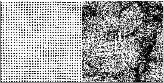
Figure 6: Evolution of the fluctuations and formation of structures in a simulation (with periodic boundary conditions, representing the infinite system case) started from a correlated and cold initial conditions. Even in this case structures form firstly on small scales and then propagate to larger and larger scales. The initial conditions are generated by applying a correlated displacement field to a pre-initial perfect cubic lattice configuration (see bsl02 ; jbruno ). One may note the appearance of “filaments”, linking clusters of particles of different sizes, marking the trace of long-range correlations in the initial particle distribution. Indeed, models of primordial density fields in the early universe predict the presence of long-range weak amplitude correlations on small scales; on large scales (i.e., $r>100$ Mpc) instead the matter distribution should have super-homogeneous (or hyper-uniform) features (see discussion in, e.g., book ; glass ; slv07 ).

The equation of motion of particle in an expanding background is then

$$\ddot{\vec{x}}_{i}+2H(t)\vec{x}_{i}=-\frac{1}{a^{3}}\sum_{i\neq j}Gm_{j}\frac{\vec{x}_{i}-\vec{x}_{j}}{|\vec{x}_{i}-\vec{x}_{j}|^{3}}$$ (14)

where the dots dots denote derivatives with respect to time, $\vec{x}_{i}$ is the comoving position of the $i^{th}$ particle, of mass $m_{i}$, related to the physical coordinate by $\vec{r}_{i}=a(t)\vec{x}_{i}$, and where $a(t)$ is the scale factor of the background cosmology with Hubble constant $H(t)=\dot{a}/a$. The static case can be obtained when $a(t)=1$ and thus $H(t)=0$. The expansion rate $a(t)$ is determined by the type of energy component which dominates the universe on large scales. For example one may consider a matter-dominated universe or the case where expansion is dominated by a cosmological constant (dark energy). In current cosmological models the $70\%$ of the energy is made of dark energy, $25\%$ of dark matter and $5\%$ of ordinary baryonic matter.

In this situation one can develop a perturbation treatment of the self-gravitating fluid equations in an expanding universe. The results are similar with the static case discussed above and in a matter-dominated universe linear theory describes a growing and a decaying mode, both of them power laws in time rather than exponential as in Eq.13. Thus in the linear regime at least, it is possible to map the evolution in a static and in an expanding universe by taking into account the different density fluctuations growth time rates.

In the non-linear regime, when cold initial conditions are considered, one observes the same general characteristics found in the static background case: a bottom-up aggregation process leading to a “self-similar” evolution of the correlation function (in the sense of Fig.4)efts88 . The time-rate of growth is power-law instead of exponential also in the non-linear regime.

The simplest approach in modeling the large scale evolution into non-linear matter structure is represented by the collapse of a single over-dense region into a self-gravitating halo via the same spherical collapse model used to study the collapse of a finite system (see e.g. peacock ; coles ). It is interesting to note that the radius of an over-dense sphere behaves in the same way as the expansion factor for a closed universe and therefore one is able to model the growth of a spherically symmetric density perturbation using the same equations as classical cosmology, i.e. the Friedmann equations.

The collapse into self-gravitating virialized objects is then a common feature to finite and infinite systems. In the context of cosmological N-body simulations the core-halo structures are simply called halos, by which it is intended the virialized part of these structures. Halos are ubiquitous in N-body simulations and they show interesting universal properties (density profiles, velocity distributions), although different from the those of the finite system described above. Even in this situation one would like to develop an analytic treatment to understand the formation of these objects and their properties. This is still lacking despite the fact that there have been several attempts for an analytical derivation of the properties of these halos, and in particular of their density and velocity profiles (see morikawa in this volume). Standard approaches are usually based on non-collisional approximations (see hansen ; white for a discussion of the subject and for a list of references).

5 Conclusions

The dynamics of infinite self-gravitating systems is a fascinating theoretical problem of out of equilibrium statistical mechanics, directly relevant both in the context of cosmology/astrophysics and, more generally, in the physics of systems with long-range interactions. We discussed some of the many problems encountered in the study of the gravitational clustering in both finite and infinite systems. We would like to stress two important open problems. The first concerns the extent to which such numerical simulations of a finite number of particles, reproduce the mean-field/Vlasov limit which is usually used to describe the evolution from a theoretical point of view. That is, the theoretical question that arises is about the validity of this collisionless limit. Another major question is that of the understanding of halo structure observed in simulations of infinite systems: while these show strongly universal characteristics, their dynamical origin is not yet understood from a theoretical point of view.

References

- (1) A. Campa, A. Giansanti, G. Morigi and F. Sylos Labini in this volume
- (2) A. Campa, in this volume
- (3) P.H. Chavanis, in this volume
- (4) D. Lynden-Bell, Mon. Not. R. Astron. Soc., 136, 101, (1967).
- (5) T. Padmanabhan, Physics Reports, 188, 285 (1990)
- (6) S. Chandrasekhar, “Principles of Stellar Dynamics”, New York: Dover, 1960
- (7) S. Chandrasekhar, Rev. Mod. Phys., 15, 1, (1943)
- (8) T. Padmanabhan, “Structure formation in the universe”, (Cambridge University Press, Cambridge, 1993)
- (9) T. Padmanabhan in “Dynamics and Thermodynamics of Systems with Long-Range Interaction”, Dauxois, S. Ruffo, E. Arimondo, M. Wilkens, eds., (Springer, Berlin 2002)
- (10) W. C. Saslaw, “Gravitational Physics of Stellar and Galactic Systems”, (Cambridge, UK: Cambridge Univ. Press, 1985)
- (11) W. C. Saslaw, “The Distribution of the Galaxies: Gravitational Clustering in Cosmology” (Cambridge, UK: Cambridge Univ. Press, 2000).
- (12) J. Binney and S. Tremaine, “Galactic Dynamics” (Princeton University Press, 1994).
- (13) P. J. E., Peebles, The Large-Scale Structure of the Universe (Princeton University Press, Princeton New Jersey, 1980)
- (14) T. Baertschiger Ph.D. Thesis (University of Geneve, Geneva, Switzerland, 2004)
- (15) J.A. Peacock, “Cosmological physics” (Cambridge University Press, Cambridge, 1999)
- (16) M. Morikawa, in this volume
- (17) M. Joyce, in this volume
- (18) W. C. Saslaw, in this volume
- (19) J. Binney and A.Knebe, Mon. Not. R. Astron. Soc., 333, 378 (2002)
- (20) J. Diemand, B. Moore, J. Stadel, and S. Kazantzidis, Mon. Not. R. Astron. Soc., 348, 977 (2004)
- (21) C. Power et al. Mon. Not. R. Astron. Soc. 338, 14 (2003)
- (22) A. Arad and P.H. Johansson Mon. Not. R. Astron. Soc. 362, 252 (2005)
- (23) J. F. Navarro, C. S. Frenk, S. D. White Astrophys. J., 490, 493 (1997)
- (24) S. H. Hansen, B. Moore, New Astron. 11 333 (2006)
- (25) V. Springel, et al., Nature, 435, 629 (2005)
- (26) G. Efstathiou, C. S. Frenk, S. D. M. White, and M. Davis, Mon. Not. R. Astr. Soc., 235, 715 (1988).
- (27) R. E. Smith et al., Mon. Not. R. Astron. Soc., 341, 1311 (2003)
- (28) A. Gabrielli, F. Sylos Labini, M. Joyce , L. Pietronero, “ Statistical physics for cosmic structures”, (Springer Verlag, Berlin, 2004)
- (29) A. Gabrielli, M. Joyce, B. Marcos, F. Sylos Labini, T. Baertschiger, Phys. Rev. E74, 021110 (2006)
- (30) A. Gabrielli, P. A. Masucci & F. Sylos Labini, Phys. Rev. E69, 031110 (2004)
- (31) A. Gabrielli, F. Sylos Labini, & S. Pellegrini, Europhys.Lett., 46, 127 (1999)
- (32) T. Baertschiger & F. Sylos Labini, Phys. Rev., D69, 123001-1 (2004)
- (33) T. Baertschiger, A. Gabrielli, M. Joyce, F. Sylos Labini, Phys. Rev.E 75, 059905 (2007)
- (34) T. Baertschiger, M. Joyce, F. Sylos Labini and B. Marcos, arXiv:0711.2219
- (35) M. Joyce, B. Marcos, A. Gabrielli, T. Baertschiger, F. Sylos Labini, Phys. Rev. Lett., 95, 011304 (2005)
- (36) B. Marcos, T. Baertschiger, M. Joyce, A. Gabrielli, F. Sylos Labini, Phys. Rev., D73, 103507 (2006)
- (37) T. Baertschiger, A. Gabrielli, M. Joyce, B. Marcos, F. Sylos Labini, Phys. Rev., E76, 011116 (2007)
- (38) F. Sylos Labini, T. Baertschiger & M. Joyce, Europhys.Lett., 66, 171 (2004)
- (39) A. Gabrielli, M. Joyce, and F. Sylos Labini, Phys. Rev., D65, 083523 (2002)
- (40) F. Sylos Labini and N. L. Vasilyev Astron. Astrophys., in the press (2007) arXiv:0710.0224
- (41) T. Baertschiger and F. Sylos Labini, Europhys.Lett., 57, 322 (2002)
- (42) M. Joyce, D. Levesque, B. Marcos, Phys.Rev., D72, 103509 (2005)
- (43) J. Peacock and S. Dodds, Mon. Not. R. Astron. Soc., 280, L19 (1996)
- (44) V. Sahni and P. Coles, Physics Reports, 262, 1 (1995).