Improving SUSY Spectrum Determinations at the LHC with the Wedgebox Technique

Abstract

The LHC has the potential not only to discover supersymmetry (SUSY), but also to permit fairly precise measurements of at least a portion of the sparticle spectrum. Proposed mass reconstruction methods rely upon either inverting invariant mass endpoint expressions or upon solving systems of mass-shell equations. These methodologies suffer from the weakness that one certain specific sparticle decay chain is assumed to account for all the events in the sample. Taking two examples of techniques utilizing mass-shell equations, it is found that also applying the wedgebox technique allows for the isolation of a purer event sample, thus avoiding errors, possibly catastrophic, due to mistaken assumptions about the decay chains involved and simultaneously improving accuracy. What is innovative is using endpoint measurements (via the wedgebox technique) to obtain a more homogeneous, well-understood sample set rather than just using said endpoints to constrain the values of the masses (here found by the mass-shell technique). The fusion of different established techniques in this manner represents a highly profitable option for LHC experimentalists who will soon have data to analyze.

1 Introduction

LHC experimentalists will soon determine whether or not Supersymmetry (SUSY) is a TeV-scale phenomenon: if so, colored sparticles will probably be the first to be discerned, possibly soon followed by neutralinos, charginos, and sleptons if favorable decay channels are open, though measuring the masses of these latter colorless sparticles with percent precision will be challenging:1999fr ; Ball:2007zza . The reason for this is that every R-parity-conserving SUSY event produces at least two invisible particles (the lightest SUSY particles, or LSPs) which carry away significant missing energy and make it impossible to reconstruct mass peaks. Therefore, many SUSY mass extraction techniques depend on precise measurement of invariant mass distribution endpoints. For a sparticle decaying into an LSP and a Standard Model (SM) fermion pair, either via a three-body decay or sequential two-body decays, it is straight-forward to see how the endpoint of the di-fermion invariant mass distribution yields the mass difference between the decaying sparticle and the LSP (perhaps modified by the on-mass-shell intermediate for two-body decays) Paige:1996nx ; Hinchliffe:1996iu ; Gianotti:682494 ; Hinchliffe:1998ys ; Hinchliffe:1999zc ; Mura:1311179 . Studies attempting to fully reconstruct the actual sparticle masses from invariant mass endpoint information rely on specific longer decay chains, typically $\widetilde{q}\to\widetilde{\chi}^{0}_{2}q\to\widetilde{\ell}^{\pm}\ell^{\mp}q\to\widetilde{\chi}^{0}_{1}\ell^{+}\ell^{-}q$ Bachacou:1999zb ; Gjelsten:2004ki ; Gjelsten:2005aw ; Gjelsten:2005sv ; Gjelsten:2005vv ; Gjelsten:708246 ; Gjelsten:2006as ; Miller:2005zp ; Lytken:703773 ; Butterworth:2007ke ; Lester:2006cf ; Allanach:2000kt ; Tovey:2003ef ; Borjanovic:2005tv ; Tovey:2008ui — each event would have two $\tilde{q}$’s (for instance) produced. It is then theoretically doable to construct enough invariant mass distributions to determine the sparticle masses; however, in practice endpoint measurement may be complicated by low event rates, fitting criteria, unaccounted-for (in the simulation) higher-order and radiativeHorsky:2008yi effects, and (in particular) backgrounds.

Ideas on how to measure SUSY masses without relying on distribution endpoints have also been put forward. The work of Nojiri et al.Nojiri:2003tu ; Kawagoe:2004rz , for example, uses mass-shell relations in a sufficiently long SUSY decay chain, e.g. $\tilde{g}\to b~{}\tilde{b}\to\widetilde{\chi}_{2}^{0}bb\to\widetilde{l}^{\pm}l^{\mp}bb\to l^{\pm}l^{\mp}bb\widetilde{\chi}_{1}^{0}$; if some of the masses are already known in this chain the others can in principle be found by solving mass-shell relations for a small sample of events, which may in fact lie far from the endpoint. Another method, due to Cheng et al.Cheng:2007xv ; Cheng:2008mg ; Cheng:2009fw , starts from very similar looking mass-shell relations, but instead of assuming some masses and solving for the others, scans the whole mass-space for points where these relations are most likely to be satisfied. Both methods, hereafter designated as ‘Mass Shell Techniques’ (MSTs), seem quite effective in obtaining percent-level determination of the sought-after SUSY masses, at least at the parameter points considered in those works.

The accuracy of both these MSTs hinges on one critical assumption: the decay topology of choice has been isolated. In the actual LHC data, the decay topology would have to be inferred, if this is at all possible, before proceeding; MSTs would thus appear to be excellent roads to SUSY mass reconstruction which, however, begin only at a point half-way to the destination.

The present work focuses on the first half of this road; i.e., isolating a desired decay topology, and on how this affects a subsequent MST analysis. As a first foray into this potentially quite thorny task, consider specific topologies studied in Nojiri:2003tu and Cheng:2007xv ; Cheng:2008mg ; Cheng:2009fw involving a pair of neutralinos $\widetilde{\chi}_{i}^{0}\widetilde{\chi}_{j}^{0}$ ($i,j=2,3,4$) that subsequently decay to leptons (electrons and muons) via on-shell sleptons. This situation is amenable to a wedgebox analysis Bisset:2005rn ; Bian:2006xx which is based upon a scatter plot of the di-electron mass $M_{e^{+}e^{-}}$ versus the dimuon mass $M_{\mu^{+}\mu^{-}}$. A key benefit of this technique is that it allows (at least partial) separation of individual events according to the specific $(i,j)$-pair whose production gave rise to them. Given sufficient statistics, events from each such decay-type fall in distinct, easily-recognized zones of the wedgebox plot. The overall topology of the resulting wedgebox plot then tests for the significant presence of the various possible $(i,j)$ decay channels — which may for instance signal the meaningful presence of a decay channel erroneously assumed to have been insignificant as the basis for a MST analysis. Events can be selected from a specific zone of the wedgebox plot, preferably a zone populated by only one decay channel. This acts to maximize sample homogeneity and assure the basic MST assumption is satisfied.

Although the wedgebox technique relies on locating the endpoints of invariant mass distributions — just like the studies Bachacou:1999zb ; Gjelsten:2004ki ; Gjelsten:2005aw ; Gjelsten:2005sv ; Gjelsten:2005vv ; Gjelsten:708246 ; Gjelsten:2006as ; Miller:2005zp ; Lytken:703773 ; Butterworth:2007ke ; Lester:2006cf ; Allanach:2000kt ; Tovey:2003ef ; Borjanovic:2005tv ; Tovey:2008ui mentioned earlier, the information sought is radically different: the wedgebox analysis is tailor-made for event sample sets comprised of assorted produced sparticle pairs and multiple sparticle decay chains. The observed endpoints serve to delineate the zones and allow for selection of purer subset(s) from an overall sample set. (Using this endpoint information to determine a set of cuts is a far more rational course than that of arbitrarily choosing some numerical cut-off values to purify the data sample.) Virtually all previous studies presume such purification has already been accomplished either by an unspecified set of cuts or a fortuitous choice of SUSY input parameters. The wedgebox technique illustrates a concrete method of how to deal with the more general case, and the consequences which result and should not be ignored in a coupled analysis aiming to extract the sparticle masses.

This paper will show that MSTs, by construction unrelated to invariant mass endpoints, can nevertheless be improved by information contained in these endpoints — specifically via the wedgebox technique. The paper is organized as follows: Sections 2 and 3 concentrate on the ‘N-MST’ method of Nojiri et al. and the ‘C-MST’ method of Cheng et al., respectively; Section 4 then offers conclusions and some additional discussion on SUSY mass spectral analyses at the LHC.

2 The N-MST Method of Nojiri et al.

For the N-MST method, the focus will be on the decay of a heavy MSSM pseudoscalar Higgs boson as considered in Nojiri:2003tu . The specific decay chain is

$$pp\to A^{0}\to\widetilde{\chi}_{i}^{0}\widetilde{\chi}_{j}^{0}\to\widetilde{l}_{1}^{\pm}{l_{1}}^{\mp}\widetilde{l}_{2}^{\pm}{l_{2}}^{\mp}\to{l_{1}}^{\mp}{l^{\prime}_{1}}^{\pm}{l_{2}}^{\mp}{l^{\prime}_{2}}^{\pm}\widetilde{\chi}_{1}^{0}\widetilde{\chi}_{1}^{0}$$ (1)

where the Higgs boson decays to neutralinos ($i,j=2,3,4$) via on-shell sleptons of the electron- or muon- variety (see Fig. 1).

Figure 1: Feynman diagram for the decay (1). Here $i,j=2,3,4$ while the label 1 or 2 on leptons stands for either $e$ or $\mu$.

Assuming the final leptons’ four-momenta are known while the LSP’s escape detection, (1) implies six mass-shell constraints on the eight unknown components of LSP four-momenta ($p^{\mu}$ and $p^{\prime\mu}$),

$$m_{\widetilde{\chi}_{1}^{0}}^{2} = p^{2}$$ (2)

$$m_{\widetilde{\chi}_{1}^{0}}^{2} = p^{\prime 2}$$ (3)

$$m_{\widetilde{l}_{1}}^{2} = (p_{l_{1}}+p)^{2}$$ (4)

$$m_{\widetilde{l}_{2}}^{2} = (p_{l_{2}}+p^{\prime})^{2}$$ (5)

$$m_{\widetilde{\chi}_{i}^{0}}^{2} = (p_{l_{1}}+p_{l^{\prime}_{1}}+p)^{2}$$ (6)

$$m_{\widetilde{\chi}_{j}^{0}}^{2} = (p_{l_{2}}+p_{l^{\prime}_{2}}+p^{\prime})^{2}$$ (7)

Nojiri et al. also posit two overall momentum conservation constraints

$$(p_{l_{1}}+p_{l_{2}}+p_{l^{\prime}_{1}}+p_{l^{\prime}_{2}}+p+p^{\prime})\cdot\vec{x} = 0$$ (8)

$$(p_{l_{1}}+p_{l_{2}}+p_{l^{\prime}_{1}}+p_{l^{\prime}_{2}}+p+p^{\prime})\cdot\vec{y} = 0$$ (9)

along directions ($x$ , $y$) transverse to the beam (the $z$-direction), though this would appear to be contingent on the Higgs boson having no transverse momentum. If all the masses $m_{\widetilde{\chi}_{1}^{0}}$, $m_{\widetilde{l}_{1}}$, $m_{\widetilde{l}_{2}}$, $m_{\widetilde{\chi}_{i}^{0}}$, and $m_{\widetilde{\chi}_{j}^{0}}$ are known in advance, one can solve the eight equations (2)-(9) for the eight unknowns and reconstruct the Higgs boson mass via

$$m_{A}^{2}=(p_{l_{1}}+p_{l_{2}}+p_{l^{\prime}_{1}}+p_{l^{\prime}_{2}}+p+p^{\prime})^{2}$$ (10)

from just one Higgs boson event of the type (1). However, even in this idealized scenario which does not include detector resolution, particle widths, backgrounds, etc., there are two major caveats which prevent this procedure from being so straightforward:

• There is a 4-fold ambiguity in assigning labels $l_{1,2},l^{\prime}_{1,2}$ to the leptons; this forms a combinatoric background.

• Combining (2)-(9) leads to a quartic equation with 0, 2 or 4 solutions for the unknown momenta.

So what one must do in practice is collect a number of events and deduce the correct value of $m_{A}$ from the maximum of the resulting distribution. In Nojiri:2003tu a $10^{3}$ event sample (with no backgrounds) thus yielded a percent-level determination of the Higgs boson mass.

2.1 Addition of the Wedgebox Technique

2.1.1 Box Topology

As shown in Nojiri:2003tu the programme sketched in the previous section works fairly well at Snowmass Benchmark SPS1a Allanach:2002nj where the dominant Higgs boson decays are via (1) with $i=j=2$. Therein, 1000 events of the type

$$pp\to A^{0}\to{\widetilde{\chi}}^{0}_{2}{\widetilde{\chi}}^{0}_{2}\to llll{\widetilde{\chi}}^{0}_{1}{\widetilde{\chi}}^{0}_{1}$$ (11)

were generated using the HERWIG6.4 Corcella:2000bw ; Corcella:2002jc ; Moretti:2002eu event generator and passed through the detector simulator package ATLFAST Richter-Was:683751 . The only cuts required were that all four isolated leptons have $\eta<2.5$, with two of the leptons also having $p_{T}~{}>~{}20\,\hbox{GeV}$ while the other two have $p_{T}~{}>~{}10\,\hbox{GeV}$. Same-flavor events such as $e^{+}e^{-}e^{+}e^{-}$ or $\mu^{+}\mu^{-}\mu^{+}\mu^{-}$ were also included if one of the two possible pairings of OS leptons in such configurations gave a di-lepton invariant mass beyond the $\sim 78\,\hbox{GeV}$ kinematic endpoint (implying the other possible pairing is the correct one). Thirty percent of the original 1000 events passed the cuts and selection criteria, leaving 300 events for the N-MST analysis, and these in turn yielded the correct Higgs boson mass with a resolution of only $6\,\hbox{GeV}$ Nojiri:2003tu .

The following set of cuts are herein adopted in a effort to reproduce these results using ISAJETBaer:1999sp ; Paige:2003mg and a detector simulation which assumes a typical LHC experiment, as provided by private programs checked against results in the literature, in place of HERWIG and ALTFAST:

1. Leptons must be hard ($p_{T}^{\ell}>10,8\,\hbox{GeV}$ for $e^{\pm},\mu^{\pm}$, respectively; $|\eta^{\ell}|<2.4\,$), and isolated (no tracks of other charged particles in a $r=0.3\,\hbox{rad}$ cone around the lepton, and less than $3\,\hbox{GeV}$ of energy deposited into the electromagnetic calorimeter for $0.05\,\hbox{rad}<r<0.3\,\hbox{rad}$ around the lepton).

2. There must be missing energy in the range: $20\,\hbox{GeV}<\hbox to0.0pt{\hbox to12.00859pt{\hfil/\hfil}\hss}E_{T}<130\,\hbox{GeV}\;$.

3. No jets are present with a reconstructed energy $E_{jet}$ greater than $50\,\hbox{GeV}$.
   

A sufficient sample of $pp\to A^{0}$ events is collected to represent an integrated LHC luminosity of $300\,\hbox{fb}^{-1}$, the same integrated luminosity as in Nojiri:2003tu , though this study only finds about 200 events of the type (11) for this luminosity. About 11% of the generated events pass the cuts and selection criteria

Fig. 2a shows the wedgebox plot at SPS1a for $pp\to A^{0}\to e^{+}e^{-}\mu^{+}\mu^{-}$ events. A ‘simple box’ topology consistent with the expected ${\widetilde{\chi}}^{0}_{2}{\widetilde{\chi}}^{0}_{2}$ origin of lepton pairs is clear. Moreover, the number of flavor-balanced events ($e^{+}e^{-}e^{+}e^{-}+\mu^{+}\mu^{-}\mu^{+}\mu^{-}+e^{+}e^{-}\mu^{+}\mu^{-}$) exceeds the number of flavor-unbalanced events ($e^{+}e^{-}e^{\pm}\mu^{\mp}+\mu^{+}\mu^{-}\mu^{\pm}e^{\mp}$) at this parameter point Huang:2008qd ; this indicates that the events come primarily from a Higgs boson decay with decay topology (1). Though the final number of events passing cuts is somewhat small (only 40 compared to the $1000\,\times 0.3\,=300$ which Nojiri:2003tu estimates, for the reasons noted above) the number of events in the distribution of solutions is quite a bit larger: recall the bulleted caveats earlier which potentially can yield a $4\times 4$ = 16-fold multiplicity factor. Though only a factor of 4 or so is observed, nonetheless a fairly clear peak in the distribution emerges (see Fig. 2b) at the correct value of $m_{A}\approx 395\,\hbox{GeV}$.

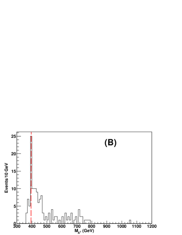
Figure 2: (A) Wedgebox plot at SPS1a ($A^{0}$ bosons only) for $300\,\hbox{fb}^{-1}$ luminosity, cuts as in text. Dotted lines show locations of kinematic endpoints from ${\widetilde{\chi}}^{0}_{2,3,4}\to{\widetilde{\chi}}^{0}_{1}$ decays. (B) Distribution of solutions for SPS1a ($A^{0}$ bosons only). Here the maximum is at the correct Higgs boson mass of $m_{A}\approx 395\,\hbox{GeV}$.

Naturally, other processes might also generate events of the signal type. It is clearly incorrect to consider only events due to $A^{0}$ production without also including $H^{0}$ production. At SPS1a, $m_{A}$ and $m_{H}$ differ by less than 3 GeV, so the $H^{0}$ events may be expected to aid in the mass determination. However, only 6 $H^{0}$ events (as compared to 40 $A^{0}$ events) are found. In addition, 16 events from direct neutralino pair production and 15 events from production processes involving charginos (these two event categories are each produced via an electroweak vector gauge boson) and/or isolated leptons from heavy-quark decays (in sparticle-containing events) contribute to the background. Standard Model processes do not contribute any events. Fig. 3a shows the wedgebox plot at SPS1a including all these event-types. Fig. 3b then shows the specific neutralino pair that is generated in each event (irrespective of the production type). While the overwhelming majority of the events are due to ${\widetilde{\chi}}^{0}_{2}{\widetilde{\chi}}^{0}_{2}$ as expected/hoped, a couple ${\widetilde{\chi}}^{0}_{2}{\widetilde{\chi}}^{0}_{3}$ events, a ${\widetilde{\chi}}^{0}_{3}{\widetilde{\chi}}^{0}_{3}$ event, and a ${\widetilde{\chi}}^{0}_{4}{\widetilde{\chi}}^{0}_{4}$ event are also present. Somewhat fortuitously, all four of these non-${\widetilde{\chi}}^{0}_{2}{\widetilde{\chi}}^{0}_{2}$ events fall outside of the ${\widetilde{\chi}}^{0}_{2}{\widetilde{\chi}}^{0}_{2}$ box region delineated by the dashed lines in the lower-left corner of Fig. 3(a,b), as do 6 of the 15 ‘Bad (mainly chargino-containing) events. Even considering possible additional experimental smearing, it should be apparent to experimentalists (who do not see color-coded events) that such events are outside of the ${\widetilde{\chi}}^{0}_{2}{\widetilde{\chi}}^{0}_{2}$ box. In this case, the inclusion or removal of these distinguishable wrong-chain events does not markedly alter the distribution of solutions shown in Fig.  3c (which is little degraded from the $A^{0}$-only plot shown in Fig. 2b). However, it does indicate how reference to the exact (within experimental accuracy) numerical value for the edges of the ${\widetilde{\chi}}^{0}_{2}{\widetilde{\chi}}^{0}_{2}$-box delivered by the wedgebox plot (or equivalently by an analysis of the two same-flavor dilepton invariant mass distributions) might aid in improving the N-MST analysis. The worth of the wedgebox information becomes more pronounced when the topology is not so simple (as is often the case for allowable MSSM parameter sets). This more general situation is addressed next.

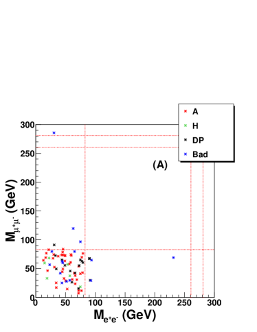
Figure 3: (A) Complete wedgebox plot for SPS1a, for $300\,\hbox{fb}^{-1}$, showing the origin of each four-lepton event — labeled as from ‘$A$’, ‘$H$’, ‘DP’(direct production), or otherwise ‘Bad’. (B) specific pair of neutralinos generated in each four-lepton event — identified as ${\widetilde{\chi}}^{0}_{2}{\widetilde{\chi}}^{0}_{2}$ (‘Z2Z2’), ${\widetilde{\chi}}^{0}_{2}{\widetilde{\chi}}^{0}_{3}$ (‘Z2Z3’), ${\widetilde{\chi}}^{0}_{3}{\widetilde{\chi}}^{0}_{3}$ (‘Z3Z3’), ${\widetilde{\chi}}^{0}_{4}{\widetilde{\chi}}^{0}_{4}$ (‘Z4Z4’), or other events-types (‘Bad’). (C) Distribution of solutions from full SPS1a event set. (D) Distribution of solutions from the SPS1a event set (inclusion or omission of events lying outside the ${\widetilde{\chi}}^{0}_{2}{\widetilde{\chi}}^{0}_{2}$-box has virtually no impact on this plot).

2.1.2 Wedge Topology

The SPS1a parameter point event set is dominated by events in which a ${\widetilde{\chi}}^{0}_{i}{\widetilde{\chi}}^{0}_{j}$ $(i=2=j=2)$ pair is generated, consistent with the expected decay chain presumed by the N-MST analysis in Nojiri:2003tu . In principle, this N-MST method should also work for a set of events for which $i\neq j$. The complication comes when one considers that the experimentalists event set (consistent with the cuts already) specified will then in general consist of a mixture of different decay chains involving different generated pairs of neutralinos. As a case in point, consider the following MSSM parameter set:

MSSM Test Point I

$$\mu=190\,\hbox{GeV}~{}~{}~{}M_{2}=280\,\hbox{GeV}~{}~{}\tan\beta=10~{}~{}M_{A}=600\,\hbox{GeV}$$

$$M_{{\widetilde{e},\widetilde{\mu}}_{L,R}}=150\,\hbox{GeV}~{}~{}M_{\widetilde{\tau}_{L,R}}=250\,\hbox{GeV}~{}~{}M_{\tilde{q},\tilde{g}}=1000\,\hbox{GeV}.$$

which has the mass spectrum shown in Table 1.

Table 1: Relevant masses at the MSSM Test Point I,II

Particle	Mass (Point I) (GeV)	Mass(Point II) (Gev)
${\widetilde{\chi}}^{0}_{1}$	$119.94$	$86.03$
${\widetilde{\chi}}^{0}_{2}$	$180.33$	$143.09$
${\widetilde{\chi}}^{0}_{3}$	$197.98$	$166.40$
${\widetilde{\chi}}^{0}_{4}$	$317.72$	$277.27$
$\widetilde{e_{R}}$	$156.17$	$127.20$
$\widetilde{\mu_{R}}$	$156.17$	$127.20$
$A^{0}$	$600.0$	$700.00$
$H^{0}$	$609.28$	$705.58$

Now the main production modes contributing to the $e^{+}e^{-}\mu^{+}\mu^{-}$ signal are the Higgs boson channels $H^{0}/A^{0}\to{\widetilde{\chi}}^{0}_{2}{\widetilde{\chi}}^{0}_{2},{\widetilde{\chi}}^{0}_{2}{\widetilde{\chi}}^{0}_{3},{\widetilde{\chi}}^{0}_{2}{\widetilde{\chi}}^{0}_{4}$, ‘direct’ neutralino pair production channels ${\widetilde{\chi}}^{0}_{2}{\widetilde{\chi}}^{0}_{3}\;\&\;{\widetilde{\chi}}^{0}_{2}{\widetilde{\chi}}^{0}_{4}$, and ‘mixed’ channels involving charginos, mainly ${\widetilde{\chi}}^{\pm}_{2}{\widetilde{\chi}}^{\mp}_{2}\;\&\;{\widetilde{\chi}}^{\pm}_{2}{\widetilde{\chi}}^{0}_{2,3,4}$ production. A random sample of $e^{+}e^{-}\mu^{+}\mu^{-}$ events will therefore not be a clean collection of Higgs boson decays, which for the luminosity considered here ($300\,\hbox{fb}^{-1}$) number about 150 against nearly 800 direct channel and 100 or so mixed channel events. This point then presents a more challenging case for applying the mass relation method.

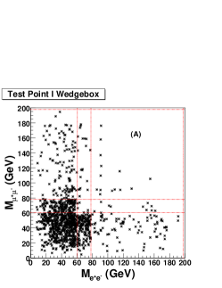
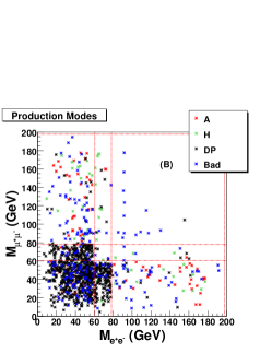
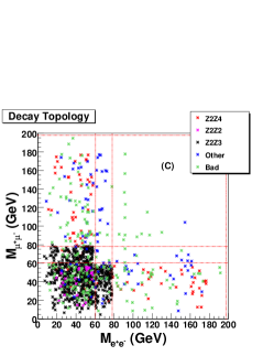
Figure 4: (A) Wedgebox plot for the MSSM Test Point I defined in the text, for $300\,\hbox{fb}^{-1}$. (B) origin of each four-lepton event labeled as from ‘$A$’, ‘$H$’, ‘DP’(direct production), or otherwise ‘Bad’. (C) specific pair of neutralinos generated in each four-lepton event identified as ${\widetilde{\chi}}^{0}_{2}{\widetilde{\chi}}^{0}_{4}$ (‘Z2Z4’), ${\widetilde{\chi}}^{0}_{2}{\widetilde{\chi}}^{0}_{3}$ (‘Z2Z3’), ${\widetilde{\chi}}^{0}_{2}{\widetilde{\chi}}^{0}_{2}$ (‘Z2Z2’), some other neutralino pair (‘Other’), or other events ‘Bad’.

However, the shape of the wedgebox plot at this point suggests selecting events via their decay topology: Fig. 4a shows a clear ’double wedge’ topology implying that events due to ${\widetilde{\chi}}^{0}_{2}{\widetilde{\chi}}^{0}_{2}$ decays are confined to the innermost box bounded by kinematic edges at $\sim 60\,\hbox{GeV}$, while those due to ${\widetilde{\chi}}^{0}_{2}{\widetilde{\chi}}^{0}_{3}$ events are enclosed in the legs of the short wedge terminating at $\sim 80\,\hbox{GeV}$. Events from ${\widetilde{\chi}}^{0}_{2}{\widetilde{\chi}}^{0}_{4}$ decays span both of these regions and beyond up to the final kinematic edge at $\sim 200\,\hbox{GeV}$.

Strictly speaking, the structure of Fig. 4a does not uniquely lead to the particle assignments noted in the previous paragraph. In the MSSM, there are other processes that can generate edges in the wedgebox topology aside from those of the form ${\widetilde{\chi}}^{0}_{j}\to l^{+}l^{-}{\widetilde{\chi}}^{0}_{1}$, including ${\widetilde{\chi}}^{\pm}_{2}\to l^{+}l^{-}{\widetilde{\chi}}^{\pm}_{1}$ and ${\widetilde{\chi}}^{0}_{j}\to l^{+}l^{-}{\widetilde{\chi}}^{0}_{2}$. The latter were given the appellation ‘stripes’ in Bisset:2005rn wherein they are discussed in some detail. For instance, in principle, the shorter (longer) wedge could be due to ${\widetilde{\chi}}^{0}_{3}\to l^{+}l^{-}{\widetilde{\chi}}^{0}_{2}$ (${\widetilde{\chi}}^{0}_{3}\to l^{+}l^{-}{\widetilde{\chi}}^{0}_{1}$) rather than due to ${\widetilde{\chi}}^{0}_{3}\to l^{+}l^{-}{\widetilde{\chi}}^{0}_{1}$ (${\widetilde{\chi}}^{0}_{4}\to l^{+}l^{-}{\widetilde{\chi}}^{0}_{1}$) as described above. Separate studies of decay kinematics can potentially exclude such alternative possibilities. For parameter set choices examined herein, these other feasible decay modes have a totally negligible effect. More importantly, as will be discussed more in the next section, such ambiguities are largely irrelevant to the mass spectrum analyses described in this work.

As in Fig. 3(b,c), Fig. 4(b,c) is color-coded to show the separate distributions of events from different production channels (A, H, or ’direct’ production $\equiv$ DP) and by their assorted neutralino-pair types; these distributions agree with remarks in the previous paragraph. Note, however, the presence of ‘Bad’ events which do not distribute themselves nicely within the kinematic bounds and which are typically due to chargino decays. Though nearly 10 percent of the total number of events are ‘Bad events, about half of these are excluded by rejecting events outside the overall wedge structure, again nicely illustrating the strength of the wedgebox technique.

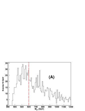
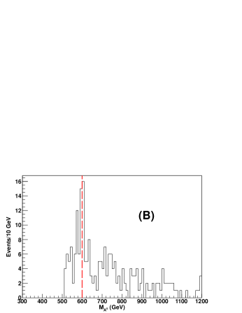
Figure 5: (A) Distribution of solutions for events taken from the inner box region of Fig. 4a; i.e., within the first set of dotted lines at $\sim 60\,\hbox{GeV}$. Here the correct Higgs boson mass of $M_{A}\approx 600\,\hbox{GeV}$ does not appear at the peak. (B) Distribution of solutions for events taken from the outer legs of Fig. 4a; i.e., within the regions bounded by dotted lines at $\sim 80\,\hbox{GeV}$ and $\sim 200\,\hbox{GeV}$. Here the correct Higgs boson mass of $M_{A}\approx 600\,\hbox{GeV}$ coincides with the peak.

Without the assistance of the wedgebox plot, one might be led to assume that events with $M_{ee,\mu\mu}<60\,\hbox{GeV}$ correspond mostly to the decay topology of (1) with $i=j=2$. This, however, leads to a Higgs boson mass distribution as shown in Fig. 5a. There is neither a clear peak nor any kind of distinguishing feature near the correct value of $M_{A}=600\,\hbox{GeV}$. Evidently, what might seem the natural choice of using events from the densest region of the wedgebox plot is not optimal.

Instead, events should be selected from the most homogeneous zone of the wedgebox plot, which in this case consists of the outermost legs from $80\,\hbox{GeV}$ to $200\,\hbox{GeV}$, corresponding mostly to $A^{0}\to{\widetilde{\chi}}^{0}_{2}{\widetilde{\chi}}^{0}_{4}$ (even without looking at Fig. 5b, Bian:2006xx predicts that events in the outer wedge of a double-wedge plot come from Higgs boson decays). As seen in Fig. 5b, the N-MST method now works splendidly, yielding an easily-identified peak at the correct Higgs boson mass, even though now an additional sparticle mass plays into the equations. The goodness of fit is more surprising considering the number of ’bad’ events distributed throughout this zone; inspection reveals that these latter, however, often fail to give solutions to equations (2)-(9), so they do not heavily interfere with the shape of the distribution.

Improvement of the N-MST method via a wedgebox plot, at least for the Higgs boson decay topology considered here, is therefore quite straightforward. However, these improvements may not always be able to counter some of the short-comings of the N-MST model, namely, the assumptions of the known sparticle masses and zero net transverse momentum — Eqns. (9). The sparticle masses are assumed to be determined via some unspecified preceding analysis, and it would be more correct to attach uncertainties to these values rather than just input the exact values given by the simulator at this point in the parameter space. It is also quite possible that the mass of the heavier neutralino $\widetilde{\chi}^{0}_{4}$ required for the analysis at MSSM Test Point I may be far less accurately determined (or left unknown) by said nameless preceding analyses than are the masses of the lighter sparticles ($\widetilde{\chi}^{0}_{1}$, $\widetilde{\chi}^{0}_{2}$, and $\tilde{\ell}^{\pm}$) which suffice at the SPS1a point. Thus a study in which both the Higgs boson mass and the mass of the heavier neutralino are simultaneously determined would certainly have merit. Better still would be to jettison reliance on such un-named previous studies and to determine all the to-date unknown beyond-the-standard-model particle masses in a self-contained analysis. This is the aim of the C-MST method to which this paper now turns (as opposed to piling more details into a fundamentally-weaker N-MST analysis). The slightly more pedagogical goal of this N-MST section has been to succinctly demonstrate the worth of a combined MST & wedgebox analysis without immediately introducing numerous subtle (and potentially distracting) issues inherent in an even more realistic and self-contained study.

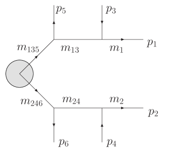
Figure 6: Event topology, taken from Cheng:2007xv ; Cheng:2008mg ; Cheng:2009fw .

3 The C-MST Method of Cheng et al.

Next consider the C-MST method. The process treated by Cheng et al. Cheng:2007xv ; Cheng:2008mg ; Cheng:2009fw is illustrated in Fig. 6 in which the masses $m_{1}$, $m_{2}$, $m_{13}$, $m_{24}$, $m_{135}$ and $m_{246}$ must satisfy a set of equations precisely analogous to (2)-(9):

$$m_{1}^{2} = p_{1}^{2}$$ (12)

$$m_{2}^{2} = p_{2}^{2}$$ (13)

$$m_{13}^{2} = \left(p_{1}+p_{3}\right)^{2}$$ (14)

$$m_{24}^{2} = \left(p_{2}+p_{4}\right)^{2}$$ (15)

$$m_{135}^{2} = \left(p_{1}+p_{3}+p_{5}\right)^{2}$$ (16)

$$m_{246}^{2} = \left(p_{2}+p_{4}+p_{6}\right)^{2}$$ (17)

$$p_{\text{sum}}^{x} = \sum_{i}p^{x}_{i}$$ (18)

$$p^{y}_{\text{sum}} = \sum_{i}p^{y}_{i}$$ (19)

where the transverse momentum sums $p_{\text{sum}}^{x,y}$ are assumed to be calculable from measurements of associated jet momenta (produced, though not shown, in the gray bubble in Fig. 6) and missing momentum (from the LSPs) necessary to balance the whole:

$$p^{x}_{\text{sum}}=\sum_{l}p^{x}_{l}+p^{x}_{\text{miss}}\qquad p^{y}_{\text{sum}}=\sum_{l}p^{y}_{l}+p^{y}_{\text{miss}}$$ (20)

The specific example considered in Cheng:2007xv ; Cheng:2008mg ; Cheng:2009fw was production of two neutralinos via squarks in the MSSM, followed by decay via on-shell smuons to muons and two LSPs:

$$\tilde{q}\tilde{q}\to q~{}q~{}\widetilde{\chi}_{2}^{0}~{}\widetilde{\chi}_{2}^{0}(\to\tilde{\mu}^{\pm}{\mu}^{\mp}\to\mu^{+}\mu^{-}\widetilde{\chi}_{1}^{0})$$ (21)

giving

$$m_{1} =m_{2}=m_{\tilde{\chi}^{0}_{1}}$$

$$m_{13} =m_{24}=m_{\tilde{\mu}}$$

$$m_{135} =m_{246}=m_{\tilde{\chi}^{0}_{2}}$$ (22)

In the three-dimensional space of masses $(m_{\widetilde{\chi}^{0}_{1}},m_{\widetilde{\chi}^{0}_{2}},m_{\widetilde{\mu}})$, each event gives eight equations (12)-(19) for the eight unknown LSP momenta $p_{1}^{\mu}$ and $p_{2}^{\mu}$, assuming the outgoing muon momenta $p_{3},p_{4},p_{5},p_{6}$ can be measured. The solution to this set of equations is again, as for the system of (2)-(9), a quartic equation with 0, 2, or 4 real roots. In contrast to the discussion of the last section, however, rather than trying to find the point in $(m_{\widetilde{\chi}^{0}_{1}},m_{\widetilde{\chi}^{0}_{2}},m_{\widetilde{\mu}})$-space where the density of solutions ($\equiv\mathbb{N}(m_{\widetilde{\chi}^{0}_{1}},m_{\widetilde{\chi}^{0}_{2}},m_{\widetilde{\mu}})$) is maximized, instead the point where the gradient of $\mathbb{N}$ is maximized (a heuristic argument for this is given in Cheng:2007xv ; Cheng:2008mg ; Cheng:2009fw ) is sought.

In Cheng:2007xv ; Cheng:2008mg ; Cheng:2009fw this method apparently works quite well at the MSSM parameter points studied, giving all relevant sparticle masses to a few percent after collection of data samples corresponding to $300\,\hbox{fb}^{-1}$ of integrated LHC luminosity. However, to test the robustness of this technique and the extent to which augmentation with the wedgebox technique can improve results, consider a new MSSM parameter point (see Tab. 1 again for masses):

MSSM Test Point II

$$\mu=-150\,\hbox{GeV}~{}~{}~{}~{}~{}~{}M_{2}=250\,\hbox{GeV}~{}~{}~{}~{}~{}~{}M_{1}=90\,\hbox{GeV}$$

$$\tan\beta=5~{}~{}~{}~{}~{}M_{\widetilde{e,\mu}_{L},\widetilde{\tau}}=250\,\hbox{GeV}~{}~{}~{}~{}~{}M_{\widetilde{e,\mu}_{R}}=120\,\hbox{GeV}$$

$$M_{A}=700\,\hbox{GeV}~{}~{}~{}~{}~{}M_{\tilde{q}}=400\,\hbox{GeV}~{}~{}~{}~{}M_{\tilde{g}}=500\,\hbox{GeV}$$

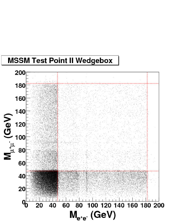
Figure 7: Wedgebox at MSSM Test Point II for a luminosity of $90\,\hbox{fb}^{-1}$.

3.1 Wedgebox selection

The wedgebox structure of Fig. 7 is again generated using ISAJET Baer:1999sp ; Paige:2003mg and the event selection criteria mentioned earlier (save no jet cut); the plot compartmentalized into four substantially event-populated regions by the shown red-dashed lines to which will be applied the following nomenclature:
The Zone 1 box, with $[M_{ee}\,\hbox{and}\,M_{\mu\mu}]<47\,\hbox{GeV}$, is the most densely-populated region of the wedgebox plot and should include all ${\widetilde{\chi}^{0}_{2}}{\widetilde{\chi}^{0}_{2}}$ events.
Zone 2 is composed of two rectangles (the legs of wedges) running outwards along both axes from the Zone 1 box — satisfying the condition that $[M_{ee}\,\hbox{and}\,M_{\mu\mu}]<182\,\hbox{GeV}$ and $[M_{ee}\,\hbox{or}\,M_{\mu\mu}\,\hbox{but not both}]<47\,\hbox{GeV}$. Events due to ${\widetilde{\chi}^{0}_{2}}{\widetilde{\chi}^{0}_{3}}$ and ${\widetilde{\chi}^{0}_{2}}{\widetilde{\chi}^{0}_{4}}$ not residing in Zone 1 will fall in Zone 2.
Zone 3, with $47\,\hbox{GeV}<[M_{ee}~{}and~{}M_{\mu\mu}]<182\,\hbox{GeV}$, lies outside of Zones 1 & 2 and should only be populated by ${\widetilde{\chi}^{0}_{3}}{\widetilde{\chi}^{0}_{3}}$, ${\widetilde{\chi}^{0}_{3}}{\widetilde{\chi}^{0}_{4}}$ and ${\widetilde{\chi}^{0}_{4}}{\widetilde{\chi}^{0}_{4}}$ events.

Figure 8: Two-dimensional mass space scan for MSSM Test Point II, seeking the point of steepest descent via the C-MST method, using the whole sample from the wedgebox plot. The axes are the difference between the input mass and the real mass of LSP and slepton.

Consider first using four-lepton events across the whole wedgebox plot — this would include several different kinds of neutralino pair events. A scan was performed over the $(m_{\widetilde{\chi}^{0}_{1}},m_{\widetilde{\chi}^{0}_{2}},m_{\widetilde{\mu}})$ mass space, and the resulting values projected onto the $(m_{\widetilde{\chi}^{0}_{1}},m_{\widetilde{\mu}})$-plane. As Table 1 shows $m_{\widetilde{\mu}}-m_{\widetilde{\chi}^{0}_{1}}\sim 41\hbox{GeV}$, Fig. 8 indicates that the gradient of $\mathbb{N}$ maximizes along the line $m_{\widetilde{\chi}^{0}_{1}}=m_{\widetilde{\mu}}$ rather than at the desired true value: the C-MST method fails badly in this attempt to find the sparticle masses. Since the wedgebox plot clearly indicates that ${\widetilde{\chi}^{0}_{2}}{\widetilde{\chi}^{0}_{3}}$, ${\widetilde{\chi}^{0}_{2}}{\widetilde{\chi}^{0}_{4}}$ and ${\widetilde{\chi}^{0}_{4}}{\widetilde{\chi}^{0}_{4}}$ production is substantial, the failure of the C-MST is not surprising given the inhomogeneity of the data set.

Consider instead performing an analysis limited to events in Zone 3 — which should be more homogeneous. Before proceeding though one more feature of the wedgebox plot should be taken into account: there is a clear $Z$-line at $[M_{ee}\,\hbox{or}\,M_{\mu\mu}]\simeq 91\,\hbox{GeV}$. This is due to neutralinos decaying to an LSP and a pair of leptons via an on-shell $Z^{0}$ rather than via a slepton. The situation is greatly simplified if the events in Zone 3 are further curtailed to encompass only those for which $100\,\hbox{GeV}<[M_{ee}\,\hbox{and}\,M_{\mu\mu}]<182\,\hbox{GeV}$. This truncated Zone 3 will be called Zone 3^′. This will exclude the on-shell $Z^{0}$ events along with those due to ${\widetilde{\chi}^{0}_{3}}{\widetilde{\chi}^{0}_{3}}$ or ${\widetilde{\chi}^{0}_{3}}{\widetilde{\chi}^{0}_{4}}$. The remaining fairly homogeneous subset of events still yields 1000+ signal events (corresponding to $90\,\hbox{fb}^{-1}$ of LHC integrated luminosity), 80% of which are in fact due to ${\tilde{\chi}^{0}_{4}}{\tilde{\chi}^{0}_{4}}$ pair production (the remainder mostly involve colored sparticle decays into the heavier chargino, $\widetilde{\chi}_{2}^{\pm}$).

At this juncture it is appropriate to revisit a statement made in the previous section — that ambiguities in identifying the particle identities from the wedgebox plot topology are largely irrelevant to the analysis to be performed. As noted in the case of MSSM Test Point I, the occurrence of ‘stripes could mean that zones of the wedgebox plot should be re-assigned. For instance, Zone 3 could be due to ${\widetilde{\chi}}^{0}_{3}\to{\widetilde{\chi}}^{0}_{1}$ decays (and thus more correctly referred to as a ${\widetilde{\chi}^{0}_{3}}{\widetilde{\chi}^{0}_{3}}$ region), while Zone 2 has many ‘stripe events — ${\widetilde{\chi}}^{0}_{3}\to{\widetilde{\chi}}^{0}_{2}$ decays. This is not true at this point in the parameter space. Since the goal is to select the region of the wedgebox plot with the purest event set, the outer-most (up and to the right) clearly delineated region is chosen to perform the analysis. Said region will never be due to stripe events — the isolated process will be of the form ${\widetilde{\chi}}^{0}_{j}\to l^{+}l^{-}{\widetilde{\chi}}^{0}_{1}$, where $j=3$ or $4$. The mass value obtained from the analysis will be correct, the only question will be whether it is $m_{{\widetilde{\chi}}^{0}_{3}}$ or $m_{{\widetilde{\chi}}^{0}_{4}}$. Further input may be required to resolve this uncertainty. Likewise, if the wedgebox plot topology was a single wedge, then the legs of the wedge could be due to ${\widetilde{\chi}^{0}_{2}}{\widetilde{\chi}^{0}_{3}}$ or ${\widetilde{\chi}^{0}_{2}}{\widetilde{\chi}^{0}_{4}}$ (in this latter case presumably something in the coupling heavily suppresses the rate for ${\widetilde{\chi}}^{0}_{3}\to l^{+}l^{-}{\widetilde{\chi}}^{0}_{1}$, and so such events make a negligible impact on the wedgebox plot). Again, an analysis of the type presented herein would yield a correct mass determination, only with some ambiguity as to the naming of the particle involved.

Additional improvements in the numerical results are possible if another piece of information is utilized: the actual value for the edge of the $\widetilde{\chi}^{0}_{4}\widetilde{\chi}^{0}_{4}$ box, $\Delta$. It is clear that this edge can be measured quite precisely via the wedgebox or the traditional one-dimensional triangular mass distribution, yielding a relation between the three masses in the equation:

$$\Delta=m_{\widetilde{\chi}^{0}_{4}}\sqrt{1-\frac{m_{\widetilde{\mu}}^{2}}{m_{\widetilde{\chi}^{0}_{4}}}^{2}}\sqrt{1-\frac{m_{\widetilde{\chi}^{0}_{1}}^{2}}{m_{\widetilde{\mu}}^{2}}}\;\;\;.$$ (23)

This additional information enables one to scan for only $m_{\widetilde{\chi}^{0}_{1}}$ and $m_{\widetilde{\mu}}$, with the $\widetilde{\chi}^{0}_{4}$ mass calculated by solving the equation above.

Proceeding somewhat gradually, first consider applying an analysis incorporating $\Delta$ to the neutralino events from Zone 3^′, but with no detector effects and with the simulation co-opted to only include correct lepton placements in Fig. 6. The result, shown in Fig. 9, indicates that the desired physical mass is indeed given quite accurately by the point of steepest descent for $\mathbb{N}$.

Figure 9: Two-dimensional scan result seeking the point of steepest descent via the C-MST method, using events from Zone 3^′ without detector effects and with correct lepton placements. The horizontal axis is the $\widetilde{\chi}^{0}_{1}$ mass, and the vertical axis is the mass difference of slepton and $\widetilde{\chi}^{0}_{1}$ The horizontal and vertical lines show the correct values for $m_{\widetilde{\mu}}-m_{\widetilde{\chi}^{0}_{1}}$ and $m_{\widetilde{\chi}^{0}_{1}}$, respectively. The triangle gives the optimal location obtained from the C-MST steepest descent analysis.

Continuing on to the more realistic Zone 3^′ analysis including detector smearing and possible lepton placement errors leads to the result shown in Fig. 10. Clearly results are worse than in Fig. 9: the point of the steepest descent of $\mathbb{N}$ is still in the neighborhood of the physical mass (there is in fact a local maximum quite close to the correct value, but it is not the global maximum indicated by the triangle), but it is obviously not a sharp maximum in the solutions space.

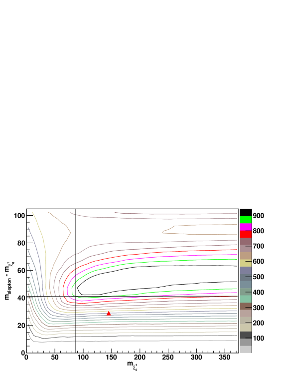
Figure 10: Two-dimensional scan result seeking the point of steepest descent via the C-MST method, using 1080 events from Zone 3^′ and also incorporating detector effects and excluding simulation information not available to the experimentalists concerning correct lepton placement. The triangle gives the optimal location obtained from the C-MST steepest descent analysis.

One reason for persisting inaccuracy is difficulty in applying the momentum conservation relation (20) — primarily due to detector smearing effects. With a simulation, one is able to compare the (’parton level’) net transverse momentum of the two neutralinos produced by the generator (prior to their decay), labeled as $p_{parton}$, to the sum of the momenta of the four leptons in the signal plus the missing momentum, designated as $p_{calc}$. If $p_{parton}$ and $p_{calc}$ actually match the quantities on the left- and right-hand sides of Eqns. (20), respectively, then they should be equal. However, as illustrated by Fig. 11, this is not the case. The difference arises from the detector smearing of the lepton momenta (in addition the smearing of the momenta of the other observed particles alters the value calculated for the missing momentum). The range of the imbalance between the experimentally-measurable value of $p_{calc}$ and the desired value of $p_{parton}$ is $-30\,\hbox{GeV}~{}\raisebox{-1.00006pt}{$\buildrel\scriptscriptstyle>\over{\scriptscriptstyle\sim}$}~{}p_{T}~{}\raisebox{-1.00006pt}{$\buildrel\scriptscriptstyle>\over{\scriptscriptstyle\sim}$}~{}30\,\hbox{GeV}$. This is formidable in light of the fact that a small inaccuracy in $p_{T}$ (say $2\,\hbox{GeV}$) can change the number of solutions at a given mass point by 10%.

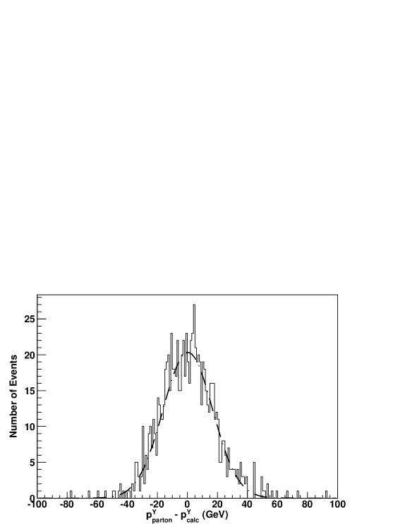
Figure 11: $p_{T}$ distribution for one of the transverse directions. Here $p_{parton}$ designated the net momentum of the two neutralinos (prior to their decay) while $p_{calc}$ is the sum of the four leptons’ momenta plus the calculated missing momentum. Thus $p_{calc}$ includes detector smearing effects. Superimposed as a dashed curve on the simulation data is a Gaussian fit whose standard deviation is $16.5\,\hbox{GeV}$ (and with a mean value of $0.3\,\hbox{GeV}$)

If smearing effects could be eliminated, so that $p_{calc}$ would essentially be equal to $p_{parton}$, fits to masses would be quite good (easily within 1%). Unfortunately, actual experiments cannot know how large the $p_{T}$ imbalance between $p_{parton}$ and $p_{calc}$ is in any given event: the best that can be done is to perform a scan over this $p_{T}$ uncertainty for each event, taking for instance $-16\,\hbox{GeV}<p_{T}<16\,\hbox{GeV}$. This is done in making Fig. 12, whose maximum does lie somewhat closer to the actual LSP mass; however, since the correct value of $m_{\widetilde{\mu}}-m_{\widetilde{\chi}^{0}_{1}}$ was assumed in this 1-D projection, the result is somewhat better than what would be obtained in practice. The fitted LSP mass in Fig. 12 has a small error but with a slightly up-biased central value (primarily due to the fact that the neutralino pairs do not have a fixed CM energy).

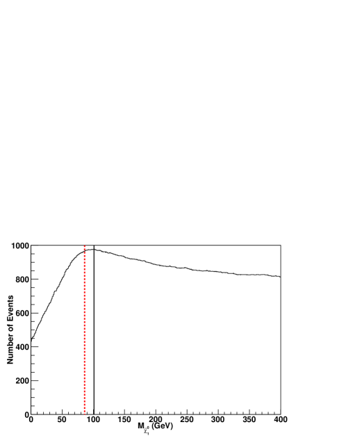
Figure 12: 1-D projection of Fig. 10, assuming the correct value of $m_{\widetilde{\mu}}-m_{\widetilde{\chi}^{0}_{1}}$, and scanning over $-16\,\hbox{GeV}<p_{T}<16\,\hbox{GeV}$. The maximum of the curve, $m_{\widetilde{\chi}^{0}_{1}}\,\simeq\,100\,\hbox{GeV}$, roughly approximates the actual LSP mass ($86\,\hbox{GeV}$), given by the red dashed line.

4 Discussion & Conclusions

Use of a wedgebox plot to select the most homogeneous sample of events has been shown to increase the accuracy and efficacy of the N-MST and C-MST mass reconstruction methods. If the events analyzed do not mostly share the same decay topology, both methods fail. A wedgebox analysis can help ascertain whether or not this is the case. If the wedgebox is a simple box, then a mass reconstruction analysis can proceed with confidence. However, over much of the allowable MSSM parameter space the topology of the wedgebox plot is not merely a lone box — if a wedge or composite structure is observed, then selecting events from the legs of the wedge or the outer areas generally proves the most effective. The outermost (more to the right, more toward the top) ‘incorporated portions of a wedgebox plot basically yield the purest data set. Here ‘incorporated portion refers to a clearly delineated zone in the plot in agreement with the predictions of the underlying model. Thus, in Fig. 7 for instance, straggler events beyond $M\simeq 183\,\hbox{GeV}$, which are not due to neutralino decays, may be eliminated. Choosing the outermost portion must be weighed against the falling number of events populating such regions (recall though that here MST requirements are relatively modest, and the need for purity generally dominates). The triangular distribution of events within the dilepton mass distributions imply that an adequately-populated portion of the wedgebox plot will be well-delineated along its outer edges — which may be taken in this MSSM analysis as indicative that the events in this region are largely from neutralino processes rather than from other process.

Note that selecting events from the legs of a wedge runs counter to the choices made in all the N-MST and C-MST publications. In Nojiri:2007pq for instance, some care is taken to describe the desirability of so-called ‘symmetric events’ — where both legs from the original parent particle contain the same intermediate particle states. The present work, on the other hand, makes the case that the benefits from using un-symmetric decay legs, e.g. efficient isolation of events with the same decay chain structure, may well trump the convenience of symmetric events in the subsequent MST analysis, and therefore unsymmetric events should not be ignored or viewed as an unnecessary complication.

The time scale required to collect a sufficient number of events to generate a wedgebox diagram is roughly comparable to that needed to perform an MST analysis. This is in spite of the fact that the wedgebox technique relies upon populating scatter plots while an MST analysis in principle only requires collection of enough events to simultaneously solve the requisite equations. In practice, ambiguity in assigning the leptons and multiple solutions to the resulting quartic equation (see bulleted items in Secn. 2 ) as well as experimental factors (also enumerated earlier) necessitate a far larger sample of events to perform either of the MST analyses discussed. Further, and even more compellingly, without augmentation by the wedgebox technique, applying an MST analysis to a quite limited data set is tantamount to wild speculation as to what SUSY channels are actually present and the results of such an analysis must be viewed most cautiously.

Scanning over the CM $p_{T}$ in a $\pm 10\,\hbox{GeV}$-window can also enhance the data analysis. Assumptions that the partonic CM has no transverse momentum (as implied by equations (9) and (20) ) are basically incorrect; while in the N-MST method this does not seem to matter, the C-MST method is much more sensitive to this parameter. An ‘averaging’ over $p_{T}$ improves the result, but perhaps a more detailed analysis should eventually be performed as the latest set of structure functions and other knowledge of QCD becomes available.

The MST analyses presented here also assume that the decay chain involved is a series of two-body decays via intermediate on-mass-shell sleptons. This need not be the case, and the on-mass-shell assumption should be tested. This however is beyond the purview of the wedgebox technique. The di-lepton distribution shapes for on- and off-shell decays are not identical Bachacou:1999zb ; Bisset:2005rn , and this could be used to distinguish between the two possibilities; however, the effects of cuts, backgrounds and a finite-sized data set must be considered. Ref. Chouridou:688033 notes that distribution shapes for on-shell (sequential two-body decays) and off-shell (three-body decays) are effectively indistinguishable for some parameter choices. Also, Ref. Kitano:2006gv finds that the shape of the di-lepton distribution may be affected by the nature of the neutralinos (the extent to which they are gauginos or higgsinos), illustrating how dynamical issues arising from the nature of the coupling involved in a decay may not be separable from purely kinematic issues associated with the relevant masses.

So an alternative to a straight-forward examination of the di-lepton distribution shape is desirable Lester:2006cf . The Decay Kinematic (DK) technique Kersting:2009ne ; Kang:2009sk ; Kang:2010hb might offer such an alternative wherein cross-correlating different invariant mass distributions resolves the on-shell vs. off-shell issue, though further studies are warranted. Another idea was put forward in Peskin:2008nw , wherein a rudimentary sketch of a very Dalitz-esque technique to look for the presence of two-body decay chains is presented — a realistic study applying this idea would be interesting. Refs. Lester:2006cf ; Lester:2005je instead champion a ‘Markov chain’ approach to analyzing the event sample where “no assumption is made about the processes causing the observed endpoints.” Supposedly then the issue of whether the sleptons are on-mass-shell or off-mass-shell is rendered moot to the more modest goal of determining a region of parameter space consistent with the data in a non-MST analysis.

The present work may be thought of as an early installment of a much grander programme to fuse all known kinematic mass reconstruction methods together. The make-up of this programme consists not only of combining fits from different methods for a static event sample set, but also of improving the composition of the event set under consideration. In the present work where the wedgebox technique is used to select (to the degree possible) events due to a specific $\widetilde{\chi}_{i}^{0}\widetilde{\chi}_{j}^{0}$ neutralino pair. Once a fairly homogeneous event sample is obtained then it becomes straightforward to apply various mass reconstruction methods and cross-check them. For example, in the case of Higgs boson decay considered here, one could try matching the N-MST results presented here to those from a study of 4-lepton invariant mass endpoints Huang:2008qd — it would be especially instructive to compare results at the SPS1a parameter point, for example, where both techniques, in the total ignorance of sparticle masses, give poor results individually, but may give a stronger result in unisonWIP2 .

An MST analysis is then an attractive option if enough mass-shell conditions can be found to match the number of mass components of the invisible final-state particles, as is the case for the LSP-generating SUSY decay chains considered herein. Further though, the present work shows how endpoint information funneled through the wedgebox technique can positively supplement such an MST analysis, as in the augmented C-MST study presented in Secn.  3. No mass-reconstruction technique is immune from possessing potentially faulty assumptions, and so coupling several complementary analysis techniques will in general improve reliability as well as accuracy.

Likewise, consideration of suitable inclusive variables, such as the $m_{T2}$ variableLester:1999tx ; Barr:2003rg ; Lester:2007fq and its variants Barr:2002ex ; Serna:2008zk , to augment either an MST study Nojiri:2007pq or an endpoint analysis Allanach:2000kt ; Tovey:2003ef ; Borjanovic:2005tv ; Tovey:2008ui ; Nojiri:2008hy ; Cho:2007dh ; Cho:2007qv ; Gripaios:2007is ; Barr:2007hy ; Ross:2007rm has been shown to be beneficial, at least in some cases. Then there is the entire array of dynamical (and thus model-dependent) information associated with cross-sections and the shapes(spread) of events plotted against one(or more) parameters. As noted earlier, kinematics can never really be totally divorced from the present dynamics. MSSM/mSUGRA studies combining information from cross-sections Lester:2005je or distribution shapes Ross:2007rm ; Gjelsten:2006tg ; Lester:2006yw with that from an endpoint analysis have also been performed and are no doubt the vanguard of many more such studies, at least if initial LHC results prove favorable. And, when those first major blocks of data from the LHC become available, application of numerous analysis techniques — including the wedgebox techniques, would be a good idea.

5 Acknowledgements

This work was supported in part by the National Natural Science Foundation of China Grant No. 10875063 to MB and RL.

References

- (1) ATLAS detector and physics performance. Technical design report. Vol. 2, . CERN-LHCC-99-15.
- (2) CMS Collaboration, G. L. Bayatian et. al., CMS technical design report, volume II: Physics performance, J. Phys. G34 (2007) 995–1579.
- (3) B. C. Allanach et. al., Measuring supersymmetric particle masses at the LHC in scenarios with baryon-number R-parity violating couplings, JHEP 03 (2001) 048, [hep-ph/0102173].
- (4) F. E. Paige, Determining SUSY particle masses at LHC, hep-ph/9609373.
- (5) I. Hinchliffe, F. E. Paige, M. D. Shapiro, J. Soderqvist, and W. Yao, Precision SUSY measurements at CERN LHC, Phys. Rev. D55 (1997) 5520–5540, [hep-ph/9610544].
- (6) F. Gianotti, Precision SUSY measurements with ATLAS: SUGRA ”Point 4”, Tech. Rep. ATL-PHYS-97-110. ATL-GE-PN-110, CERN, Geneva, Sep, 1997.
- (7) I. Hinchliffe and F. E. Paige, Measurements in gauge mediated SUSY breaking models at LHC, Phys. Rev. D60 (1999) 095002, [hep-ph/9812233].
- (8) I. Hinchliffe and F. E. Paige, Measurements in SUGRA models with large tan(beta) at LHC, Phys. Rev. D61 (2000) 095011, [hep-ph/9907519].
- (9) B. Mura and L. Feld, Determination of Neutralino Masses with the CMS Experiment. oai:cds.cern.ch:1311179. PhD thesis, Aachen, Tech. Hochsch., Aachen, 2006. Presented on Dec 2006.
- (10) H. Bachacou, I. Hinchliffe, and F. E. Paige, Measurements of masses in SUGRA models at CERN LHC, Phys. Rev. D62 (2000) 015009, [hep-ph/9907518].
- (11) B. K. Gjelsten, D. J. Miller, 2, and P. Osland, Measurement of SUSY masses via cascade decays for SPS 1a, JHEP 12 (2004) 003, [hep-ph/0410303].
- (12) B. K. Gjelsten, D. J. Miller, 2, and P. Osland, Measurement of the gluino mass via cascade decays for SPS 1a, JHEP 06 (2005) 015, [hep-ph/0501033].
- (13) B. K. Gjelsten, D. J. Miller, 2, and P. Osland, Resolving ambiguities in mass determinations at future colliders, hep-ph/0507232.
- (14) B. K. Gjelsten, D. J. Miller, 2, and P. Osland, Determining masses of supersymmetric particles, hep-ph/0511008.
- (15) B. K. Gjelsten, E. Lytken, D. J. Miller, P. Osland, and G. Polesello, A detailed analysis of the measurement of susy masses with the atlas detector at the lhc, Tech. Rep. ATL-PHYS-2004-007, CERN, Geneva, Jan, 2004. Contribution to the proceedings : LHC/LC workshop.
- (16) B. K. Gjelsten, D. J. Miller, 2, P. Osland, and A. R. Raklev, Mass ambiguities in cascade decays, hep-ph/0611080.
- (17) D. J. Miller, 2, P. Osland, and A. R. Raklev, Invariant mass distributions in cascade decays, JHEP 03 (2006) 034, [hep-ph/0510356].
- (18) E. Lytken, Derivation of some kinematical formulas in susy decay chains, Tech. Rep. ATL-PHYS-2005-003. ATL-COM-PHYS-2004-001, CERN, Geneva, 2004.
- (19) J. M. Butterworth, J. R. Ellis, and A. R. Raklev, Reconstructing sparticle mass spectra using hadronic decays, JHEP 05 (2007) 033, [hep-ph/0702150].
- (20) C. G. Lester, M. A. Parker, and M. J. White, 2, Three body kinematic endpoints in SUSY models with non- universal Higgs masses, JHEP 10 (2007) 051, [hep-ph/0609298].
- (21) B. C. Allanach, C. G. Lester, M. A. Parker, and B. R. Webber, Measuring sparticle masses in non-universal string inspired models at the LHC, JHEP 09 (2000) 004, [hep-ph/0007009].
- (22) D. R. Tovey, Measurement of the neutralino mass, Czech. J. Phys. 54 (2004) A175–A182.
- (23) I. Borjanovic, J. Krstic, and D. Popovic, SUSY studies with Snowmass Point 5 mSUGRA parameters, Czech. J. Phys. 55 (2005) B793–B799.
- (24) D. R. Tovey, On measuring the masses of pair-produced semi-invisibly decaying particles at hadron colliders, JHEP 04 (2008) 034, [arXiv:0802.2879].
- (25) R. Horsky, M. Kramer, 1, A. Muck, and P. M. Zerwas, Squark Cascade Decays to Charginos/Neutralinos: Gluon Radiation, Phys. Rev. D78 (2008) 035004, [arXiv:0803.2603].
- (26) M. M. Nojiri, G. Polesello, and D. R. Tovey, Proposal for a new reconstruction technique for SUSY processes at the LHC, hep-ph/0312317.
- (27) K. Kawagoe, M. M. Nojiri, and G. Polesello, A new SUSY mass reconstruction method at the CERN LHC, Phys. Rev. D71 (2005) 035008, [hep-ph/0410160].
- (28) H.-C. Cheng, J. F. Gunion, Z. Han, G. Marandella, and B. McElrath, Mass Determination in SUSY-like Events with Missing Energy, JHEP 12 (2007) 076, [arXiv:0707.0030].
- (29) H.-C. Cheng, D. Engelhardt, J. F. Gunion, Z. Han, and B. McElrath, Accurate Mass Determinations in Decay Chains with Missing Energy, Phys. Rev. Lett. 100 (2008) 252001, [arXiv:0802.4290].
- (30) H.-C. Cheng, J. F. Gunion, Z. Han, and B. McElrath, Accurate Mass Determinations in Decay Chains with Missing Energy: II, Phys. Rev. D80 (2009) 035020, [arXiv:0905.1344].
- (31) M. M. Nojiri, G. Polesello, and D. R. Tovey, A hybrid method for determining SUSY particle masses at the LHC with fully identified cascade decays, JHEP 05 (2008) 014, [arXiv:0712.2718].
- (32) Y. Bai and H.-C. Cheng, Identifying Dark Matter Event Topologies at the LHC, arXiv:1012.1863.
- (33) M. Bisset et. al., Pair-produced heavy particle topologies: MSSM neutralino properties at the LHC from gluino / squark cascade decays, Eur. Phys. J. C45 (2006) 477–492, [hep-ph/0501157].
- (34) G. Bian, M. Bisset, N. Kersting, Y. Liu, and X. Wang, Wedgebox analysis of four-lepton events from neutralino pair production at the LHC, Eur. Phys. J. C53 (2008) 429–446, [hep-ph/0611316].
- (35) B. C. Allanach et. al., The Snowmass points and slopes: Benchmarks for SUSY searches, Eur. Phys. J. C25 (2002) 113–123, [hep-ph/0202233].
- (36) G. Corcella et. al., HERWIG 6.5: an event generator for Hadron Emission Reactions With Interfering Gluons (including supersymmetric processes), JHEP 01 (2001) 010, [hep-ph/0011363].
- (37) G. Corcella et. al., HERWIG 6.5 release note, hep-ph/0210213.
- (38) S. Moretti, K. Odagiri, P. Richardson, M. H. Seymour, and B. R. Webber, Implementation of supersymmetric processes in the HERWIG event generator, JHEP 04 (2002) 028, [hep-ph/0204123].
- (39) E. Richter-Was, D. Froidevaux, and L. Poggioli, Atlfast 2.0 a fast simulation package for atlas, Tech. Rep. ATL-PHYS-98-131, CERN, Geneva, Nov, 1998.
- (40) H. Baer, F. E. Paige, S. D. Protopopescu, and X. Tata, ISAJET 7.48: A Monte Carlo event generator for p p, anti-p p, and e+ e- reactions, hep-ph/0001086.
- (41) F. E. Paige, S. D. Protopopescu, H. Baer, and X. Tata, ISAJET 7.69: A Monte Carlo event generator for p p, anti-p p, and e+ e- reactions, hep-ph/0312045.
- (42) T. Sjostrand, S. Mrenna, and P. Z. Skands, PYTHIA 6.4 Physics and Manual, JHEP 05 (2006) 026, [hep-ph/0603175].
- (43) J. Conway.
- (44) D. Stump, J. Huston, J. Pumplin, W.-K. Tung, H. Lai, et. al., Inclusive jet production, parton distributions, and the search for new physics, JHEP 0310 (2003) 046, [hep-ph/0303013].
- (45) P. Huang, N. Kersting, and H. H. Yang, Model-Independent SUSY Masses from 4-Lepton Kinematic Invariants at the LHC, Phys. Rev. D77 (2008) 075011, [arXiv:0801.0041].
- (46) R. H. K. Kadala, P. G. Mercadante, J. K. Mizukoshi, and X. Tata, Heavy-flavour tagging and the supersymmetry reach of the CERN Large Hadron Collider, Eur. Phys. J. C56 (2008) 511–528, [arXiv:0803.0001].
- (47) R. Lu and M. Bisset. Work in progress.
- (48) S. Chouridou, R. Ströhmer, and T. M. Trefzger, Study of the three body matrix element of the neutralino decay 034, Tech. Rep. ATL-PHYS-2003-034, CERN, Geneva, Jul, 2002.
- (49) R. Kitano and Y. Nomura, Supersymmetry, naturalness, and signatures at the LHC, Phys. Rev. D73 (2006) 095004, [hep-ph/0602096].
- (50) N. Kersting, A Simple Mass Reconstruction Technique for SUSY particles at the LHC, Phys. Rev. D79 (2009) 095018, [arXiv:0901.2765].
- (51) Z. Kang, N. Kersting, S. Kraml, A. R. Raklev, and M. J. White, Neutralino Reconstruction at the LHC from Decay-frame Kinematics, Eur. Phys. J. C70 (2010) 271–283, [arXiv:0908.1550].
- (52) Z. Kang, N. Kersting, and M. White, Mass Estimation without using MET in early LHC data, arXiv:1007.0382.
- (53) M. E. Peskin, Supersymmetry in Elementary Particle Physics, arXiv:0801.1928.
- (54) C. G. Lester, M. A. Parker, and M. J. White, 2, Determining SUSY model parameters and masses at the LHC using cross-sections, kinematic edges and other observables, JHEP 01 (2006) 080, [hep-ph/0508143].
- (55) N. Kersting. Work in progress.
- (56) C. G. Lester and D. J. Summers, Measuring masses of semiinvisibly decaying particles pair produced at hadron colliders, Phys. Lett. B463 (1999) 99–103, [hep-ph/9906349].
- (57) A. Barr, C. Lester, and P. Stephens, m(T2) : The Truth behind the glamour, J. Phys. G29 (2003) 2343–2363, [hep-ph/0304226].
- (58) C. Lester and A. Barr, MTGEN : Mass scale measurements in pair-production at colliders, JHEP 12 (2007) 102, [arXiv:0708.1028].
- (59) A. J. Barr, C. G. Lester, M. A. Parker, B. C. Allanach, and P. Richardson, Discovering anomaly-mediated supersymmetry at the LHC, JHEP 03 (2003) 045, [hep-ph/0208214].
- (60) M. Serna, A short comparison between and , JHEP 06 (2008) 004, [arXiv:0804.3344].
- (61) M. M. Nojiri, Y. Shimizu, S. Okada, and K. Kawagoe, Inclusive transverse mass analysis for squark and gluino mass determination, JHEP 06 (2008) 035, [arXiv:0802.2412].
- (62) W. S. Cho, K. Choi, Y. G. Kim, and C. B. Park, Measuring superparticle masses at hadron collider using the transverse mass kink, JHEP 02 (2008) 035, [arXiv:0711.4526].
- (63) W. S. Cho, K. Choi, Y. G. Kim, and C. B. Park, Gluino Stransverse Mass, Phys. Rev. Lett. 100 (2008) 171801, [arXiv:0709.0288].
- (64) B. Gripaios, Transverse Observables and Mass Determination at Hadron Colliders, JHEP 02 (2008) 053, [arXiv:0709.2740].
- (65) A. J. Barr, B. Gripaios, and C. G. Lester, Weighing Wimps with Kinks at Colliders: Invisible Particle Mass Measurements from Endpoints, JHEP 02 (2008) 014, [arXiv:0711.4008].
- (66) G. G. Ross and M. Serna, Mass Determination of New States at Hadron Colliders, Phys. Lett. B665 (2008) 212–218, [arXiv:0712.0943].
- (67) B. K. Gjelsten, D. J. Miller, 2, P. Osland, and A. R. Raklev, Mass Determination in Cascade Decays Using Shape Formulas, AIP Conf. Proc. 903 (2007) 257–260, [hep-ph/0611259].
- (68) C. G. Lester, Constrained invariant mass distributions in cascade decays: The shape of the ’m(qll)-threshold’ and similar distributions, Phys. Lett. B655 (2007) 39–44, [hep-ph/0603171].