Representation theory for vector electromagnetic beams

Abstract

A representation theory of finite electromagnetic beams in free space is formulated by factorizing the field vector of the plane-wave component into a $3\times 2$ mapping matrix and a 2-component Jones-like vector. The mapping matrix has one degree of freedom that can be described by the azimuthal angle of a fixed unit vector with respect to the wave vector. This degree of freedom allows us to find out such a beam solution in which every plane-wave component is specified by the same fixed unit vector $\mathbf{I}$ and has the same normalized Jones-like vector. The angle $\theta_{I}$ between the fixed unit vector and the propagation axis acts as a parameter that describes the vectorial property of the beam. The impact of $\theta_{I}$ is investigated on a beam of angular-spectrum field scalar that is independent of the azimuthal angle. The field vector in position space is calculated in the first-order approximation under the paraxial condition. A transverse effect is found that a beam of elliptically-polarized angular spectrum is displaced from the center in the direction that is perpendicular to the plane formed by the fixed unit vector and the propagation axis. The expression of the transverse displacement is obtained. Its paraxial approximation is also given.

I Introduction

The representation formalism and propagation characteristics of an electromagnetic beam in free space has drawn much attention Lax-LM ; Pattanayak-A ; Davis ; Davis-P1 ; Davis-P2 ; Gori-GP ; Durnin-ME ; Jordan-H ; Tovar-C ; Enderlein-P ; Seshadri ; Li1 after the advent of masers and lasers Green-W ; Kogelnik ; Kogelnik-L . It was shown Lax-LM that a linearly polarized beam solution is not compatible with the Maxwell equations, because it does not satisfy the transversality condition. It was also shown Pattanayak-A that the state of polarization is not a global property of a finite beam. Rather it is local and changes on propagation. In an attempt to describe the vectorial property of a beam, a unit vector was once introduced and was first supposed Pattanayak-A ; Davis to be perpendicular to the propagation axis. Later on, it was further pointed out Davis-P1 ; Davis-P2 that the unit vector can also be parallel to the propagation axis. Under the paraxial condition, the beam in the former case is uniformly polarized, and the beam in the latter case is now known as the cylindrical vector beam Youngworth-B1 ; Li1 . The conversion from uniformly polarized beams to cylindrical vector beams has been experimentally realized Tidwell-FK ; Stalder-S ; Youngworth-B1 ; Bomzon-BKH ; Ren-LW .

Recently, there appeared a controversy Onoda-MN1 ; Bliokh-B1 ; Bliokh-B2 over the physical properties of the light beams that were proposed to investigate the Imbert-Fedorov effect, a transverse displacement of a reflected Fedorov ; Imbert ; Pillon-GG ; Fedoseev1 ; Fedoseev2 or a transmitted Schilling ; Fedoseev1 ; Fedoseev2 ; Onoda-MN2 ; Hosten-K beam taking place at a dielectric interface. On the one hand, Onoda et. al. Onoda-MN1 disagreed with Bliokh and Bliokh Bliokh-B1 on their incident beam. On the other hand, Bliokh and Bliokh Bliokh-B2 found that the physical properties of Onoda’s incident beam Onoda-MN1 depend on the “incidence angle”. Such a controversy concerns in fact the description of the vectorial property of a finite beam.

In this paper, I will show that the vectorial property of a finite beam can be described by a parameter, the angle between a unit vector and the propagation axis. This is achieved by factorizing the field vector of a plane wave into a $3\times 2$ mapping matrix (MM) and a 2-component Jones-like vector Li2 ; Li1 ; Jones and investigating the degree of freedom of the MM. It is shown in Section II that the MM can not be determined uniquely by the transversality condition. It has one degree of freedom. The degree of freedom can be represented by the azimuthal angle of a fixed unit vector with respect to the wave vector. The idea of MM is generalized in Section III to a finite beam. For an arbitrary electromagnetic beam, each plane wave component may have its own MM and Jones-like vector. But the degree of freedom of the MM allows us to find out such a beam solution in which every plane wave component is specified by the same fixed unit vector and has the same normalized Jones-like vector. In this case, the beam as a whole has its own MM, which maps the normalized Jones-like vector to the field vector. The case of a transverse unit vector corresponds to the representation formalism discussed in Refs. Pattanayak-A ; Davis , and the case of a longitudinal unit vector corresponds to the representation formalism discussed in Refs. Davis-P1 ; Davis-P2 . The impact of the angle between the unit vector and the propagation axis is investigated in Section IV. The field vector in the first-order approximation under the paraxial condition is calculated for an angular-spectrum field scalar that is independent of the azimuthal angle. The controversy over the incident beams of Refs. Onoda-MN1 and Bliokh-B1 is resolved. A transverse effect is also found that a beam of elliptically polarized angular spectrum is displaced from the center in the direction that is perpendicular to the plane formed by the unit vector and the propagation axis. The origin of this effect is discussed. Conclusions and remarks are given in Section V.

II Degree of freedom of the mapping matrix

II.1 Mapping matrix and the existence of one degree of freedom

In a source-free position space, the electric-field vector $\mathbf{F}(\mathbf{x})$ of a monochromatic finite electromagnetic beam satisfies the transversality condition,

$$\nabla\cdot\mathbf{F}(\mathbf{x})=0.$$ (1)

The plane-wave angular-spectrum expression of the field vector, varying according to $\exp(-i\omega t)$ with the time, can be written as

$$\mathbf{F}(\mathbf{x})=\frac{1}{2\pi}\int\int_{k_{x}^{2}+k_{y}^{2}\leq k^{2}}\mathbf{f}(k_{x},k_{y})\exp(i\mathbf{k}\cdot\mathbf{x})dk_{x}dk_{y},$$ (2)

where $\mathbf{k}=k_{x}\mathbf{e}_{x}+k_{y}\mathbf{e}_{y}+k_{z}\mathbf{e}_{z}\equiv\left(\begin{array}[]{c}k_{x}\\ k_{y}\\ k_{z}\end{array}\right)$ is the wave vector satisfying $k_{x}^{2}+k_{y}^{2}+k_{z}^{2}=k^{2}$, $\mathbf{f}=\left(\begin{array}[]{c}f_{x}\\ f_{y}\\ f_{z}\end{array}\right)$ is the electric-field vector of the angular spectrum, and $\mathbf{e}_{j}$ ($j=x,y,z$) is the unit vector of the $j$-axis. According to the transversality condition (1), $\mathbf{f}$ has only two mutually orthogonal polarization states, each of them being orthogonal to $\mathbf{k}$. Denoting respectively by $p$ and $s$ the two orthogonal linearly-polarized states, we can decompose $\mathbf{f}$ as

$$\mathbf{f}=\mathbf{f}_{p}+\mathbf{f}_{s}=f_{p}\mathbf{p}+f_{s}\mathbf{s},$$ (3)

where $f_{p}$ and $f_{s}$ are respectively the $p$- and $s$-polarized complex amplitudes constituting a 2-component Jones-like vector Li2 ; Li1 ; Jones

$$\tilde{f}\equiv\left(\begin{array}[]{c}f_{p}\\ f_{s}\end{array}\right),$$ (4)

$\mathbf{p}$ and $\mathbf{s}$ are respectively the $p$- and $s$-polarized unit vectors. To be clear, we assume in this paper that both $\mathbf{p}$ and $\mathbf{s}$ are real unit vectors. We can always do this as one may see from Eq. (3). They satisfy

$$\left\{\begin{array}[]{rcl}\mathbf{p}\cdot\mathbf{k}&=&0,\\ \mathbf{s}\cdot\mathbf{k}&=&0,\end{array}\right.$$ (5)

as well as

$$\left\{\begin{array}[]{rcl}\mathbf{p}\cdot\mathbf{p}&=&1,\\ \mathbf{s}\cdot\mathbf{s}&=&1,\\ \mathbf{p}\cdot\mathbf{s}&=&0.\end{array}\right.$$ (6)

Eq. (3) means that the 3-component field vector is an element of a 2D space, rather than an element of a 3D space. Since the space of 2-component Jones-like vectors is a 2D space, Eq. (3) defines in fact a mapping from the Jones-like-vector space to the 3-component 2D space. In order to describe this mapping, we change the form of Eq. (3) into

$$\mathbf{f}=m\tilde{f},$$ (7)

where

$$m=\left(\begin{array}[]{cc}p_{x}&s_{x}\\ p_{y}&s_{y}\\ p_{z}&s_{z}\end{array}\right)$$ (8)

is the $3\times 2$ MM.

Any MM, the column vectors of which satisfy Eqs. (5) and (6), guarantees that the field vector $\mathbf{f}$ given by Eq. (7) satisfies the transversality condition whatever the Jones-like vector $\tilde{f}$ may be. But there are only five equations to determine the six unknown elements of the MM. This shows that after the transversality condition is taken into account, the MM still has one degree of freedom. That is to say, the transversality condition itself is not sufficient to determine an electromagnetic wave from a given Jones-like vector.

II.2 Description of the degree of freedom and its unique role

It is well known Green-W ; Pattanayak-A ; Davis-P2 ; Onoda-MN1 that if the unit vectors $\mathbf{p}$ and $\mathbf{s}$ are defined from the wave vector $\mathbf{k}$ in terms of an arbitrary fixed real unit vector $\mathbf{I}$ as

$$\left\{\begin{array}[]{rcl}\mathbf{p}&=&\mathbf{s}\times\frac{\mathbf{k}}{k},\\ \mathbf{s}&=&\frac{\mathbf{k}\times\mathbf{I}}{|\mathbf{k}\times\mathbf{I}|},\end{array}\right.$$ (9)

then they satisfy Eqs. (5) and (6). One might conclude that the degree of freedom is the unit vector $\mathbf{I}$. This is obviously not true, because we need two independent variables to determine the orientation of a real unit vector in a 3D space. But we can indeed use the real unit vector $\mathbf{I}$ to denote the degree of freedom somehow. To show this, let us look at a particular wave vector $\mathbf{k}$ and the unit vectors $\mathbf{p}$ and $\mathbf{s}$ that are defined by Eqs. (9) in terms of a fixed unit vector $\mathbf{I}$ as is schematically depicted in Fig. 1. It can be seen from this figure that the rotation of $\mathbf{I}$ around $\mathbf{k}$ by changing the azimuthal angle $\Theta$ of $\mathbf{I}$ with respect to $\mathbf{k}$ alters the orientation of $\mathbf{p}$ and $\mathbf{s}$. On the other hand, the rotation of $\mathbf{I}$ around $\mathbf{s}$ by changing the polar angle $\Phi$ of $\mathbf{I}$ with respect to $\mathbf{k}$ does not alter the orientation of $\mathbf{p}$ and $\mathbf{s}$. So it is the azimuthal angle $\Theta$ that plays the role of the degree of freedom and uniquely determines the MM. For a particular wave vector, different values of $\Theta$ represent different mapping matrices, and vice versa. The rotation of $\mathbf{I}$ around $\mathbf{s}$ forms a group $G(\Theta)$ that corresponds to one single value of the degree of freedom.

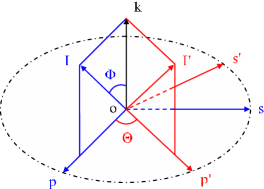
Figure 1: (Color online) The degree of freedom of the MM is denoted by the azimuthal angle $\Theta$ of $\mathbf{I}$ with respect to $\mathbf{k}$.

Based on the above description of the MM’s degree of freedom, it is concluded that different mapping matrices map a given Jones-like vector to different field vectors.

III Representation formalism for a finite beam

On factorizing the field vector of a plane wave into the MM and the Jones-like vector, we have identified one degree of freedom of the MM and shown that it can be described by the azimuthal angle of a fixed unit vector with respect to the wave vector. But we have not made any requirements on the Jones-like vector. A finite beam consists of an infinite number of plane waves. For an arbitrary beam, each plane-wave component may have its own MM and Jones-like vector. But the degree of freedom of the MM allows us to find out such a kind of beams in which every plane-wave component is specified by the same fixed unit vector and have the same normalized Jones-like vector. In the following I will put forward the representation formalism of those beams.

Assume that the fixed unit vector $\mathbf{I}$ that is common to all the plane-wave components lies in the plane $zox$ and makes an angle $\theta_{I}$ with the $z$-axis, the propagation axis,

$$\mathbf{I}(\theta_{I})=\mathbf{e}_{z}\cos\theta_{I}+\mathbf{e}_{x}\sin\theta_{I},$$ (10)

so that the MM of the plane-wave component takes the form of

$$m=\frac{1}{k|\mathbf{k}\times\mathbf{I}|}\left(\begin{array}[]{cc}(k_{y}^{2}+k_{z}^{2})\sin\theta_{I}-k_{z}k_{x}\cos\theta_{I}&kk_{y}\cos\theta_{I}\\ -k_{y}(k_{z}\cos\theta_{I}+k_{x}\sin\theta_{I})&k(k_{z}\sin\theta_{I}-k_{x}\cos\theta_{I})\\ (k_{x}^{2}+k_{y}^{2})\cos\theta_{I}-k_{z}k_{x}\sin\theta_{I}&-kk_{y}\sin\theta_{I}\end{array}\right),$$ (11)

where

$$|\mathbf{k}\times\mathbf{I}|=[k^{2}-(k_{z}\cos\theta_{I}+k_{x}\sin\theta_{I})^{2}]^{1/2}.$$ (12)

It should be noted that a given $\theta_{I}$ corresponds to the same value of the MM’s degree of freedom for each of those wave vectors that also lie in the $zox$ plane as was shown before in Fig. 1. Such a feature of $\theta_{I}$ will produce a very interesting transverse effect as will be shown in Section IV.

As discussed before, the field vector $\mathbf{f}$ of the angular spectrum is factorized by Eq. (7) into the MM (11) and the Jones-like vector,

$$\tilde{f}=\tilde{\alpha}f,$$ (13)

where $\tilde{\alpha}=\left(\begin{array}[]{c}\alpha_{p}\\ \alpha_{s}\end{array}\right)$ is the normalized Jones-like vector describing the polarization state of the angular spectrum, $\alpha_{p}$ and $\alpha_{s}$ are complex numbers satisfying the normalization condition,

$$|\alpha_{p}|^{2}+|\alpha_{s}|^{2}=1,$$ (14)

and $f$ is referred to as the field scalar of the angular spectrum. If $\tilde{\alpha}$ is common to all the plane-wave components, the electric-field vector (2) takes the following factorized form,

$$\mathbf{F}(\mathbf{x})=M(\mathbf{x})\tilde{\alpha},$$ (15)

where

$$M(\mathbf{x})=\frac{1}{2\pi}\int\int mf\exp(i\mathbf{k}\cdot\mathbf{x})dk_{x}dk_{y}$$ (16)

is the MM for the beam, and the integration limit ${k_{x}^{2}+k_{y}^{2}\leq k^{2}}$ is omitted for brevity. Eq. (15) states that the field vector in position space is the result of the mapping of the normalized Jones-like vector by the MM (16). Given a normalized Jones-like vector, altering only $\theta_{I}$ that is involved in the MM (16) will change the vectorial property of the beam. That is to say, $\theta_{I}$ behaves as a parameter that describes the vectorial property of the beam. It is not necessarily equal to $\frac{\pi}{2}$ Pattanayak-A ; Davis nor equal to $0$ Davis-P1 ; Davis-P2 .

In a circular cylindrical system with the $z$-axis being the symmetry axis, the integral (16) is changed into

$$M(\mathbf{x})=\frac{1}{2\pi}\int_{0}^{k}\int_{0}^{2\pi}mf\exp(i\mathbf{k}\cdot\mathbf{x})k_{\rho}dk_{\rho}d\varphi,$$ (17)

where $\mathbf{x}=\mathbf{r}+z\mathbf{e}_{z}$, $\mathbf{r}=r\mathbf{e}_{r}=\mathbf{e}_{x}r\cos\phi+\mathbf{e}_{y}r\sin\phi$, $\mathbf{e}_{r}$ and $\mathbf{e}_{\phi}$ are respectively the unit vectors in the radial and azimuthal directions in position space; correspondingly, $\mathbf{k}=\mathbf{k}_{\rho}+k_{z}\mathbf{e}_{z}$, $\mathbf{k}_{\rho}=k_{\rho}\mathbf{e}_{\rho}=k_{x}\mathbf{e}_{x}+k_{y}\mathbf{e}_{y}$, $k_{x}=k_{\rho}\cos\varphi$, $k_{y}=k_{\rho}\sin\varphi$, $k_{z}=(k^{2}-k_{\rho}^{2})^{1/2}$, $\mathbf{e}_{\rho}$ and $\mathbf{e}_{\varphi}$ are respectively the unit vectors in the radial and azimuthal directions in wave-vector space.

IV Impact of angle $\theta_{I}$ on the properties of a finite beam

Eq. (15) together with Eq. (17) in the circular cylindrical system is an exact beam solution to the Maxwell equations in free space. It does not rely on the paraxial condition, and the field scalar $f=f({k_{\rho},\varphi})$ can be any physically allowed function of $k_{\rho}$ and $\varphi$. In this section we are concerned with the impact of angle $\theta_{I}$ on the properties of a beam and therefore consider only such a field scalar $f=f(k_{\rho})$ that is $\varphi$-independent, sharply peaked at $k_{\rho}=0$, and square-integrable. Furthermore, due to the relation $\mathbf{I}(\theta_{I}+\pi)=-\mathbf{I}(\theta_{I})$, it is enough to assume $|\theta_{I}|\leq\frac{\pi}{2}$. In the following, the $\theta_{I}$ will be confined to this interval.

IV.1 Field vector distribution in the first-order approximation

A sharply peaked field scalar $f(k_{\rho})$ around $k_{\rho}=0$ means that the half divergence angle $\Delta\theta$ of the beam satisfies

$$\Delta\theta\ll\frac{1}{2\pi}.$$ (18)

Upon considering integral (17), $\frac{k_{\rho}}{k}$ in the MM can be regarded as a small number in comparison with unity. So the elements of the MM can be expanded as a power series in $\frac{k_{\rho}}{k}$. When $\theta_{I}$ is either equal to $\frac{\pi}{2}$ Lax-LM or to $0$ Li1 , the lowest correction to the zeroth-order transverse component is a second-order term remark . In this subsection, I will show that when $\theta_{I}$ satisfies

$$\Delta\theta\ll|\theta_{I}|\leq\frac{\pi}{2},$$ (19)

the transverse component will have a $\theta_{I}$-dependent first-order correction.

We rewrite Eq. (12) as

$$|\mathbf{k}\times\mathbf{I}|=|k_{z}\sin\theta_{I}|\left(1-2\frac{k_{x}}{k_{z}}\cot\theta_{I}+\frac{k_{x}^{2}\cos^{2}\theta_{I}+k_{y}^{2}}{k_{z}^{2}\sin^{2}\theta_{I}}\right)^{1/2}.$$

The condition (19) guarantees that the second and the third parts in the second factor are the first-order and the second-order terms in comparison with the first part. As a result, in the first-order approximation, we have for the MM,

$$m\approx m_{0}+m_{1},$$ (20)

where

$$m_{0}=\mathrm{sgn}(\theta_{I})\left(\begin{array}[]{cc}1&0\\ 0&1\\ 0&0\end{array}\right)$$

is the zeroth-order term,

$$m_{1}=\mathrm{sgn}(\theta_{I})\left(\begin{array}[]{cc}0&\cot\theta_{I}\sin\varphi\\ -\cot\theta_{I}\sin\varphi&0\\ -\cos\varphi&-\sin\varphi\end{array}\right)\frac{k_{\rho}}{k}$$

is the first-order correction, and $\mathrm{sgn}$ is the sign function. Substituting Eq. (20) into Eqs. (15) and (17) yields the field vector,

$$\mathbf{F}(\mathbf{x})\approx\mathbf{F}_{T}^{(0)}(\mathbf{x})+\mathbf{F}_{T}^{(1)}(\mathbf{x})+\mathbf{F}_{L}^{(1)}(\mathbf{x}),$$ (21)

where

$$\mathbf{F}_{T}^{(0)}(\mathbf{x})=m_{0}\tilde{\alpha}F_{0}(r,z)$$ (22)

is the zeroth-order term that is transverse and uniformly polarized,

$$\mathbf{F}_{T}^{(1)}(\mathbf{x})=i\mathrm{sgn}(\theta_{I})(\alpha_{s}\mathbf{e}_{x}-\alpha_{p}\mathbf{e}_{y})\frac{y}{r}F_{1}(r,z)\cot\theta_{I}$$ (23)

is the first-order correction to the transverse component which is also uniformly polarized but is $\theta_{I}$-dependent,

$$\mathbf{F}_{L}^{(1)}(\mathbf{x})=-i\mathrm{sgn}(\theta_{I})\mathbf{e}_{z}\frac{\alpha_{p}x+\alpha_{s}y}{r}F_{1}(r,z)\equiv F_{L}^{(1)}\mathbf{e}_{z}$$ (24)

is the longitudinal component,

$$F_{0}(r,z)=\int_{0}^{k}f(k_{\rho})\exp(ik_{z}z)J_{0}(rk_{\rho})k_{\rho}dk_{\rho},$$

and

$$F_{1}(r,z)=\int_{0}^{k}\frac{k_{\rho}}{k}f(k_{\rho})\exp(ik_{z}z)J_{1}(rk_{\rho})k_{\rho}dk_{\rho}.$$

In deriving Eq. (21), I have made use of the following expansion,

$$\exp(i\rho\cos\psi)=\sum_{m=-\infty}^{\infty}i^{m}J_{m}(\rho)\exp(im\psi),$$ (25)

where $J_{m}$’s are the Bessel functions of the first kind.

It is noticed that the polarization state of the first-order transverse term is different from that of the zeroth-order transverse term. As a matter of fact, they are orthogonal to each other. Combining Eqs. (22) and (23) together, we get the transverse component of the electric-field vector,

$$\mathbf{F}_{T}(\mathbf{x})=\mathrm{sgn}(\theta_{I})\left[(\alpha_{p}F_{0}+i\alpha_{s}\frac{y}{r}F_{1}\cot\theta_{I})\mathbf{e}_{x}+(\alpha_{s}F_{0}-i\alpha_{p}\frac{y}{r}F_{1}\cot\theta_{I})\mathbf{e}_{y}\right].$$ (26)

This shows that the transverse component of the beam is not in general uniformly polarized. The local polarization state is dependent on the value of $\theta_{I}$.

When $|\theta_{I}|=\frac{\pi}{2}$, the first-order correction to the transverse component vanishes, $\mathbf{F}_{T}^{(1)}(\mathbf{x})=0$. In this case the zeroth-order term of the transverse component is the field vector of uniformly-polarized beams, the polarization state being the same as that of the angular spectrum, $\tilde{\alpha}$. It satisfies, together with the first-order longitudinal component (24), the approximate transversality condition Lax-LM ,

$$\nabla_{T}\cdot\mathbf{F}_{T}^{(0)}+ikF_{L}^{(1)}=0,$$ (27)

where $\nabla_{T}=\mathbf{e}_{x}\frac{\partial}{\partial x}+\mathbf{e}_{y}\frac{\partial}{\partial y}$.

Defining $m_{c}=\frac{\alpha_{s}}{\alpha_{p}}$ and choosing $\alpha_{p}=-\frac{1}{(1+|m_{c}|^{2})^{1/2}}$ by use of the normalization condition (14), we find for the unit field vector of the angular spectrum,

$$\frac{\mathbf{f}}{|\mathbf{f}|}=-\mathrm{sgn}(\theta_{I})\frac{(1+m_{c}\frac{k_{y}}{k}\cot\theta_{I})\mathbf{e}_{x}+(m_{c}-\frac{k_{y}}{k}\cot\theta_{I})\mathbf{e}_{y}-(\frac{k_{x}}{k}+m_{c}\frac{k_{y}}{k})\mathbf{e}_{z}}{(1+|m_{c}|^{2})^{1/2}}.$$ (28)

When $\theta_{I}=-\theta$ with $\theta>0$, Eq. (28) turns into

$$\frac{\mathbf{f}}{|\mathbf{f}|}=\frac{(1-m_{c}\frac{k_{y}}{k}\cot\theta)\mathbf{e}_{x}+(m_{c}+\frac{k_{y}}{k}\cot\theta)\mathbf{e}_{y}-(\frac{k_{x}}{k}+m_{c}\frac{k_{y}}{k})\mathbf{e}_{z}}{(1+|m_{c}|^{2})^{1/2}},$$ (29)

which is the same as the equation (20) of Ref. Bliokh-B2 if $\theta$ is interpreted as the incidence angle. This shows that the incident beam of Ref. Onoda-MN1 can be described in this representation formalism as the first-order approximation of such a special beam the unit vector $\mathbf{I}$ of which happens to make an angle of the minus incidence angle with the propagation axis and happens to be normal to the interface. This is implied in Ref. Onoda-MN1 by the unit vector $\mathbf{n}$ that plays the role of $\mathbf{I}$ and explains why the physical properties of the incident beam in Ref. Onoda-MN1 depend on the “incidence angle” Bliokh-B2 . A similar incident beam was once proposed by Schilling Schilling .

Furthermore, when $\theta=\frac{\pi}{2}$, Eq. (29) reduces to

$$\frac{\mathbf{f}}{|\mathbf{f}|}=\frac{\mathbf{e}_{x}+m_{c}\mathbf{e}_{y}-(\frac{k_{x}}{k}+m_{c}\frac{k_{y}}{k})\mathbf{e}_{z}}{(1+|m_{c}|^{2})^{1/2}}.$$ (30)

Upon noticing that $m_{c}=\frac{f_{y}}{f_{x}}$ in this case, Eq. (30) is exactly the same as the equation (22) of Ref. Bliokh-B2 . This shows that the incident beam of Ref. Bliokh-B1 is nothing but the fundamental Gaussian beam, as long as the first-order longitudinal component is taken into account.

IV.2 Transverse effect

Now we are ready to discuss a transverse effect. When $|\theta_{I}|$ is not equal to $\frac{\pi}{2}$, the first-order term of the transverse component does not vanish. Since this term is not axisymmetric as is clearly shown by Eq. (23), its interference with the zeroth-order term renders the intensity distribution deformed from the axisymmetry as can be seen from Eq. (26). A direct consequence of this deformation is the following transverse effect: the barycenter of a beam of elliptically polarized angular spectrum is displaced from the center in the transverse $y$-direction; the displacement is dependent on the value of $\theta_{I}$ and on the polarization ellipticity of the angular spectrum.

To show this, let us define the $y$-position $y_{b}$ of the beam’s barycenter as the expectation of the $y$-coordinate of the beam,

$$y_{b}=\langle y\rangle=\frac{\int\int\mathbf{F}^{{\dagger}}y\mathbf{F}dxdy}{\int\int\mathbf{F}^{{\dagger}}\mathbf{F}dxdy},$$ (31)

where superscript ${\dagger}$ stands for the conjugate transpose. According to Eq. (2), we have

$$\int\int\mathbf{F}^{{\dagger}}y\mathbf{F}dxdy=\int\int(i\mathbf{f}^{{\dagger}}\frac{\partial\mathbf{f}}{\partial k_{y}}+z\frac{k_{y}}{k_{z}}\mathbf{f}^{{\dagger}}\mathbf{f})dk_{x}dk_{y}$$

and

$$\int\int\mathbf{F}^{{\dagger}}\mathbf{F}dxdy=\int\int\mathbf{f}^{{\dagger}}\mathbf{f}dk_{x}dk_{y}.$$

Furthermore, Eqs. (7) and (13) tell us that

$$\mathbf{f}^{{\dagger}}\mathbf{f}=|f|^{2}$$

and

$$\mathbf{f}^{{\dagger}}\frac{\partial\mathbf{f}}{\partial k_{y}}=f^{*}\frac{\partial f}{\partial k_{y}}+\tilde{\alpha}^{{\dagger}}m^{T}\frac{\partial m}{\partial k_{y}}\tilde{\alpha}|f|^{2}.$$

Substituting all these into Eq. (31) and noticing that $f$ is an even function of $k_{y}$, we obtain

$$y_{b}=i\frac{\int\int\tilde{\alpha}^{{\dagger}}m^{T}\frac{\partial m}{\partial k_{y}}\tilde{\alpha}|f|^{2}dk_{x}dk_{y}}{\int\int|f|^{2}dk_{x}dk_{y}},$$ (32)

which shows that the $y$-position of the beam’s barycenter is independent of $z$. Substituting Eq. (11) and $\tilde{\alpha}$, we get

$$y_{b}=-\frac{\sigma\cot\theta_{I}}{2\int_{0}^{k}|f(k_{\rho})|^{2}k_{\rho}dk_{\rho}}\int_{0}^{k}\left(1+\frac{k_{z}-k\cos\theta_{I}}{|k_{z}-k\cos\theta_{I}|}\right)\frac{|f(k_{\rho})|^{2}}{k_{z}}k_{\rho}dk_{\rho},$$ (33)

where $\sigma=-i(\alpha_{p}^{*}\alpha_{s}-\alpha_{p}\alpha_{s}^{*})$ is the polarization ellipticity of the angular spectrum. It is emphasized that this expression has a validity that does not depend on the paraxial condition (18) and large angle condition (19). It is inferred from the expression that

(1) the beam is indeed displaced a distance transversely from the center, because $y_{b}$ does not change on propagation;

(2) the opposite ellipticity $\sigma$ corresponds to the opposite displacement for a given $\theta_{I}$;

(3) the opposite angle $\theta_{I}$ corresponds to the opposite displacement for a given $\sigma$.

Let us now discuss the dependence of the transverse displacement on the angle $\theta_{I}$. If $|\theta_{I}|=\frac{\pi}{2}$, the first factor $\cot\theta_{I}$ of Eq. (33) tells us that the displacement is equal to zero. This is the case that corresponds to the uniformly polarized beams (22) in the zeroth-order approximation. If $\theta_{I}=0$, the second term in the integrand cancels the first one, also resulting in zero displacement. In fact, this case corresponds to the cylindrical vector beams which are axially symmetric in both polarization and intensity distribution Li1 . For a $\theta_{I}$ that is neither equal to $\frac{\pi}{2}$ nor equal to $0$, Eq. (33) is rewritten as

$$y_{b}=-\frac{\sigma\cot\theta_{I}}{2\int_{0}^{k}|f|^{2}k_{\rho}dk_{\rho}}\left(\int_{0}^{k}\frac{|f|^{2}}{k_{z}}k_{\rho}dk_{\rho}+\int_{0}^{k\sin|\theta_{I}|}\frac{|f|^{2}}{k_{z}}k_{\rho}dk_{\rho}-\int_{k\sin|\theta_{I}|}^{k}\frac{|f|^{2}}{k_{z}}k_{\rho}dk_{\rho}\right).$$ (34)

If $|\theta_{I}|\gg\Delta\theta$, the third integral is much smaller than the second one, remembering that $f(k_{\rho})$ is a sharply peaked function about $k_{\rho}=0$. As a result, the transverse displacement in this case becomes

$$y_{b}\approx-\frac{\sigma\cot\theta_{I}}{\int_{0}^{k}|f|^{2}k_{\rho}dk_{\rho}}\int_{0}^{k}\frac{|f|^{2}}{k_{z}}k_{\rho}dk_{\rho}.$$

Under the paraxial condition which means $k_{z}\approx k$ for the denominator of the integrand in the first-order approximation with respect to $\frac{k_{\rho}}{k}$, it reduces to

$$y_{b}\approx-\frac{\sigma}{k}\cot\theta_{I}.$$ (35)

Due to the factor $\cot\theta_{I}$ in Eq. (34), the smaller $|\theta_{I}|$ goes, the larger the magnitude of the displacement becomes until the following relation establishes,

$$\int_{0}^{k\sin|\theta_{I}|}\frac{|f|^{2}}{k_{z}}k_{\rho}dk_{\rho}=\int_{k\sin|\theta_{I}|}^{k}\frac{|f|^{2}}{k_{z}}k_{\rho}dk_{\rho}.$$ (36)

At this point, the third integral of Eq. (34) cancels the second one, and the displacement takes the form of

$$y_{b}=-\frac{\sigma\cot\theta_{I0}}{2\int_{0}^{k}|f|^{2}k_{\rho}dk_{\rho}}\int_{0}^{k}\frac{|f|^{2}}{k_{z}}k_{\rho}dk_{\rho},$$ (37)

where $\theta_{I0}$ is the solution to Eq. (36). Similarly it reduces to, under the paraxial condition,

$$y_{b}\approx-\frac{\sigma\cot\theta_{I0}}{2k}.$$

If $|\theta_{I}|$ goes even smaller, the third integral outstrips the second one in magnitude, and the displacement becomes smaller in magnitude until $\theta_{I}=0$ when the displacement is equal to zero. It is thus expected that Eq. (37) represents the maximum displacement if only the change of $\theta_{I}$ is considered. Roughly speaking, the value of $|\theta_{I0}|$ that satisfies Eq. (36) is approximately equal to the half divergence angle of the beam, $|\theta_{I0}|\sim\Delta\theta=\frac{1}{kw_{0}}$, where $w_{0}$ is the half width of the beam. For a paraxial beam in which $\Delta\theta$ is very small, the maximum transverse displacement can be as large as the order of $w_{0}$ Li3 , $|y_{b}|\approx\frac{w_{0}}{2}$, for circularly polarized angular spectra $\sigma=\pm 1$.

It is interesting to note that Schilling Schilling once found the transverse displacement more than 40 years ago for an incident beam the unit field vector of which can be described by Eq. (29). Recently, Bliokh and Bliokh Bliokh-B2 rediscovered Schilling’s result when comparing the incident beams of Refs. Onoda-MN1 and Bliokh-B1 .

V Conclusions and Remarks

In conclusion, I factorized in Eq. (7) the field vector of a beam’s angular spectrum into the MM and the Jones-like vector and showed that the degree of freedom of the MM can be described by the azimuthal angle of a fixed unit vector with respect to the wave vector. This degree of freedom provides us with such a beam solution in which every plane-wave component is specified by the same fixed unit vector $\mathbf{I}$ and has the same normalized Jones-like vector $\tilde{\alpha}$. The integral representation for the MM of a beam’s field vector was formulated in Eq. (16) [or (17) in the circular cylindrical system] by letting the unit vector lie in the plane $zox$ and make an angle $\theta_{I}$ with the $z$-axis.

The impact of the angle $\theta_{I}$ was discussed on the vectorial property of a beam that has a $\varphi$-independent field scalar $f(k_{\rho})$. The electric-field vector (21) was obtained in the first-order approximation under the paraxial condition (18) for large $|\theta_{I}|$ that satisfies Eq. (19). It was shown that the transverse component has a $\theta_{I}$-dependent first-order correction. This is different from the cases of $|\theta_{I}|=\frac{\pi}{2}$ and $\theta_{I}=0$ in which the lowest correction to the zeroth-order transverse component is a second-order term. A transverse effect was found and the dependence of the transverse displacement on $\theta_{I}$ was discussed. The paraxial approximation of the transverse displacement was also given. In a word, the angle $\theta_{I}$ in the representation formalism advanced here plays the role of a parameter that describes the vectorial property of the beam.

A physically allowed field scalar $f(k_{\rho},\varphi)$ in Eq. (17) can be expanded as a Fourier series,

$$f(k_{\rho},\varphi)=\sum_{l=-\infty}^{\infty}f_{l}(k_{\rho})\exp(il\varphi).$$ (38)

One may consider the constituent term of the following form,

$$f(k_{\rho},\varphi)=f_{l}(k_{\rho})\exp(il\varphi),$$ (39)

and discuss the impact of angle $\theta_{I}$ on the resultant beam. It is expected that when $\theta_{I}=\pm\frac{\pi}{2}$, Eq. (39) together with Eqs. (15) and (17) will yield the eigen beam of the orbital angular momentum Allen-BSW in the zeroth-order approximation.

According to the triad relation expressed by the first equation of (9) and the principle of duality in free space Davis-P1 , I would like to point out that the following $3\times 2$ matrix

$$m_{M}=\left(\begin{array}[]{cc}s_{x}&-p_{x}\\ s_{y}&-p_{y}\\ s_{z}&-p_{z}\end{array}\right)$$ (40)

can be regarded as the MM for the magnetic-field vector, which maps a Jones-like vector to the 3-component magnetic-field vector for a particular wave vector.

The representation formalism of finite electromagnetic beams developed in this paper depends closely on the MM and its degree of freedom. It is worth noting that in this representation formalism, the Jones-like vector does not depend on the MM’s degree of freedom. Therefore one Jones-like vector can be mapped to an infinite number of field vectors due to the MM’s degree of freedom, as can be seen from Eq. (7) as well as Eq. (15). The physical significance of the MM’s degree of freedom needs further investigation.

References

- (1) M. Lax, W. H. Louisell, and W. B. McKnight, Phys. Rev. A 11, 1365 (1975).
- (2) D. N. Pattanayak and G. P. Agrawal, Phys. Rev. A 22, 1159 (1980).
- (3) L. W. Davis, Phys. Rev. A 19, 1177 (1979).
- (4) L. W. Davis and G. Patsakos, Opt. Lett. 6, 22 (1981).
- (5) L. W. Davis and G. Patsakos, Phys. Rev. A 26, 3702 (1982).
- (6) F. Gori, G. Guattari, and C. Padovani, Opt. Commun. 64, 491 (1987).
- (7) J. Durnin, J. J. Miceli Jr., and J. H. Eberly, Phys. Rev. Lett. 58, 1499 (1987).
- (8) R. H. Jordan and D. G. Hall, Opt. Lett. 19, 427 (1994).
- (9) A. A. Tovar and G. H. Clark, J. Opt. Soc. Am. A 14, 3333 (1997).
- (10) J. Enderlein and F. Pampaloni, J. Opt. Soc. Am. A 21, 1553 (2004).
- (11) S. R. Seshadri, J. Opt. Soc. Am. A 24, 2837 (2007).
- (12) C.-F. Li, Opt. Lett. 32, 3543 (2007).
- (13) H. S. Green and E. Wolf, Proc. Phys. Soc. London Sec. A 66, 1129 (1953).
- (14) H. Kogelnik, Appl. Opt. 4, 1562 (1965).
- (15) H. Kogelnik and T. Li, Appl. Opt. 5, 1550 (1966).
- (16) K. S. Youngworth and T. G. Brown, Opt. Express 7, 77 (2000).
- (17) S. C. Tidwell, D. H. Ford, and W. D. Kimura, Appl. Opt. 29, 2234 (1990).
- (18) M. Stalder and M. Schadt, Opt. Lett. 21, 1948 (1996).
- (19) Z. Bomzon, G. Biener, V. Kleiner, and E. Hasman, Opt. Lett. 27, 285 (2002).
- (20) H. Ren, Y.-H. Lin, and S.-T. Wu, Appl. Phys. Lett. 89, 051114 (2006).
- (21) M. Onoda, S. Murakami, and N. Nagaosa, Phys. Rev. E 74, 066610 (2006).
- (22) K. Yu. Bliokh and Yu. P. Bliokh, Phys. Rev. Lett. 96, 073903 (2006).
- (23) K. Yu. Bliokh and Yu. P. Bliokh, Phys. Rev. E 75, 066609 (2007).
- (24) F. I. Fedorov, Dokl. Akad. Nauk SSSR 105, 465 (1955).
- (25) C. Imbert, Phys. Rev. D 5, 787 (1972).
- (26) F. Pillon, H. Gilles, and S. Girard, Appl. Opt. 43, 1863 (2004).
- (27) V. G. Fedoseev, Opt. Spektrosk. 71, 829 (1991) [Opt. Spectrosc. 71, 483 (1991)].
- (28) V. G. Fedoseev, Opt. Spektrosk. 71, 992 (1991) [Opt. Spectrosc. 71, 570 (1991)].
- (29) H. Schilling, Ann. Phys. (Leipzig) 16, 122 (1965).
- (30) M. Onoda, S. Murakami, N. Nagaosa, Phys. Rev. Lett. 93, 083901 (2004).
- (31) O. Hosten and P. Kwiat, Science 319, 787 (2008).
- (32) R. C. Jones, J. Opt. Soc. Am. 31, 488 (1941).
- (33) C.-F. Li, Phys. Rev. A 76, 013811 (2007).
- (34) If which corresponds to the TE beam mode Davis-P1 , the transverse component has only the zeroth-order term Li1 .
- (35) C.-F. Li, http://arxiv.org/abs/0707.0971v2.
- (36) L. Allen, M. W. Beijersbergen, R. J. C. Spreeuw, and J. P. Woerdman, Phys. Rev. A 45, 8185 (1992).