Thermal Conductivity from Core and Well log Data

Abstract

The relationships between thermal conductivity and other petrophysical properties have been analysed for a borehole drilled in a Tertiary Flysch sequence. We establish equations that permit us to predict rock thermal conductivity from logging data. A regression analysis of thermal conductivity, bulk density, and sonic velocity yields thermal conductivity with an average accuracy of better than 0.2 W(m K)^-1. As a second step, logging data is used to compute a lithological depth profile, which in turn is used to calculate a thermal conductivity profile. From a comparison of the conductivity-depth profile and the laboratory data it can be concluded that thermal conductivity can be computed with an accuracy of less than 0.3 W(m K)^-1 from conventional wireline data. The comparison of two different models shows that this approach can be practical even if old and incomplete logging data is used. The results can be used to infer thermal conductivity for boreholes without appropriate core data that are drilled in a similar geological setting.

1 Introduction

The German Molasse Basin is currently analysed with geothermal methods in order to determine groundwater flow rates in the deep subsurface Clauser2002 . This requires to determine accurately and separate from each other the effects of the different heat transport processes: Steady-state conductive, transient conductive, and advective heat flow. Computing the steady-state conductive temperature field requires detailed thermal conductivity data. Two requirements should be met: First, lateral variations in thermal conductivity have to be known accurately for regional studies. Second, a detailed analysis of a particular borehole requires a high resolution thermal conductivity profile. Core material in that area is either confined to a few boreholes or available only for a particular layer. This violates both requirements. Logging data, on the other hand, offer better spatial coverage and depth resolution. In a situation with an incomplete coring sequence this helps to prevent biased sampling in lithologies not representative of the full sequence. It is therefore highly desirable to derive thermal properties from logging data to improve the sparse geothermal database.

Methods to compute thermal conductivity from wireline logs can be classified into two main categories Beardsmore2001 . The first approach relates one or more logging measurements or some derived property directly to thermal properties via empirical relationships. This method has been used to compute thermal conductivity in several studies Doveton1997 ; Vacquier1988 ; Evans1977 ; Goss1975_prediction and a review is given in Blackwell1989 . In the second approach, the major mineral or rock components are identified and the volumetric fractions of these components are derived from regular wireline data. This composition together with component thermal conductivity values is then used to compute the effective thermal conductivity assuming an appropriate mixing law Williams1990 ; Brigaud1990 ; Demongodin1991 . This approach is more flexible than the first one. For instance, it does not require the same suite of logs in each borehole as long as they are suitable to compute component volumes.

It has been pointed out Goss1975_prediction ; Blackwell1989 that results of the current methods are confined to a geographic region or geological setting. In the following we would like to assess the two different methods discussed above for the Molasse Basin. As the area was explored for hydrocarbons in the past, logging data often are old and comprise only sonic or natural gamma logs. Although it would be more desirable to use only the second approach, it is necessary to evaluate direct methods as well to make full use of the available logging data. We test direct methods on a set of core data, that was analysed in the laboratory and the compositional approach using the same set of laboratory data together with wireline data obtained in the borehole.

2 Core data

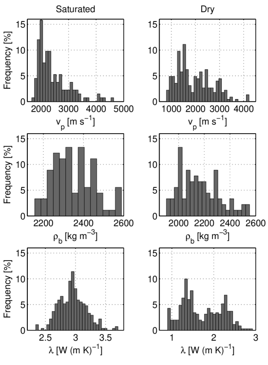
Figure 1: Histograms of sonic velocity $v_{p}$, bulk density $\rho_{b}$, and thermal conductivity $\lambda$ measured in the laboratory on core samples. Properties measured are from top to bottom: sonic velocity, bulk density, and thermal conductivity. Values are shown for saturated (left) and dry (right) conditions. The bimodal distribution corresponds to the occurrence of two different lithologies in the borehole (see also figure 7).

The data set for laboratory analysis is obtained from a borehole drilled for hot water into the Upper Marine Molasse formation. This formation consists of shaly sandstones and marls. The borehole was cored between 570–810 m depth with nearly 100 % recovery. The sequence consists of a succession of shaly sandstones and marl beds. Porosity ranges from 10–30 %. Split cores were available for measurements in sections of 1 m length. In general, we analysed every fifth section, but in some depth intervals we studied all cores. The cores had broken into several pieces during coring and splitting. We selected two to five samples from each core section for further analysis. The samples were dried at 60°C to prevent cracking or alteration of clay minerals. We measured thermal conductivity, sonic velocity, and bulk density on the dried samples. Then the samples were saturated under vacuum and the same measurements were repeated for the saturated samples. Because the samples were not well consolidated a number of samples was damaged or destroyed during saturation, resulting in a lower number of saturated measurements. Figure 1 shows histograms of the results.

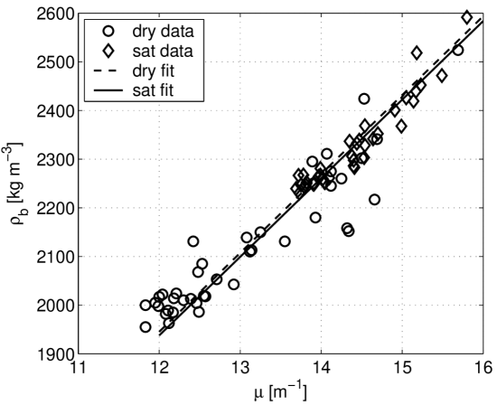
Figure 2: Calibration of bulk density measurements. The absorption coefficient $\mu$ measured on dry and saturated samples is converted into bulk density using equation 1.

Thermal conductivity was measured using the optical scanning technique which yields a continuous profile of thermal conductivity along the core axis of the sample (Popov1997, ; Popov1999, ; Surma2003, ). We also measured thermal conductivity perpendicular to the core axis to obtain anisotropy. Anisotropy ratios were generally less than 3–4 % so that we assume the rock to be isotropic. Values for each sample were computed as averages of the scanning line. We measured bulk density and sonic velocity with a multi-sensor core-logger (e. g. Weber1997a ). The measurement is performed perpendicular to the core axis. Both bulk density and sonic velocity records need special attention before they can be used in the analysis. Bulk density is measured by gamma-ray absorption mainly due to Compton scattering Ellis1987 . It is calibrated routinely using an aluminium standard. Since electron density is measured rather than real density, better results are obtained when using a calibration standard with a similar electron density (Ellis1987, ). Therefore we measured bulk density and porosity independently on a number samples using either Archimedes´ method or gas-state and solid-state pyknometers. The obtained bulk density is then plotted versus the absorption coefficient $\mu$ measured with the core-logger for dry and saturated samples. Figure 2 shows that a linear relationship exists which can be used for calibration. For dry and saturated measurements the following equations are obtained:

$$\rho_{b,s} = 161.5\mu_{s}\qquad\mathrm{(saturated)}$$ (1)

$$\rho_{b,d} = 162.1\mu_{d}\qquad\mathrm{(dry)}$$

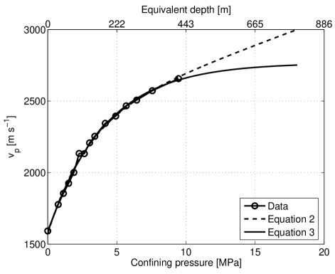
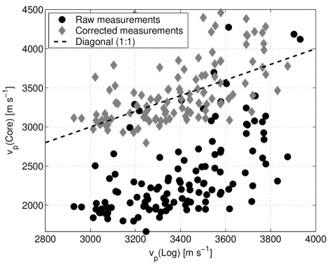
Figure 3: Variation of sonic velocity with confining pressure. Top: Laboratory data together with linear-exponential and exponential fit. The quality of the fit differs only in the extrapolated range. Bottom: Data before and after pressure correction based on equation 3.

The slope is slightly lower for saturated measurements. A detailed analysis shows that saturated gamma density should be corrected using a separate porosity measurement Hearst2000 . However, considering the data scatter and the limited range of the saturated measurements this can be included in the single calibration factor. Sonic velocity was measured on the samples under ambient pressure and we found a large difference in velocity obtained from wireline logs and cores (Figure 3, bottom panel). It is well known that changes in pressure have a profound influence on elastic properties (e. g. Mayr2002 ; Zimmerman1986 ). An empirical relationship with linear and exponential terms is usually used to correct this effect. In order to quantify the correction, sonic velocity was measured on a sample under uniaxial pressure as described in Mayr2002 . We fitted two exponential equations to this data (Figure 3), both with an exponential term but one without a linear term . The following coefficients were obtained, with pressure $P$ in MPa and velocity $v$ in  m s^-1:

$$v(p) = 2360+787\e^{0.356P}+35.7P$$ (2)

$$v(p) = 2760+1180\e^{0.243P}$$ (3)

The rms-errors are 19 m s^-1 (eq. 2) and 18 m s^-1 (eq. 3). Both equations fit the pressure-velocity data equally well and differ only in the extrapolated range from 450 m to 820 m. This is, however, the depth range of the samples and equation 3 yields better results when we compare corrected laboratory data to logging data. Equation 2 slightly over-corrects the laboratory data. This is probably caused by the fact that the measurements only cover a range of up to 10 MPa. In this pressure range the exponential term is more significant, and the linear term is not well defined. Therefore, we used equation 3 to correct the measurements (Figure 3, lower part). The remaining scatter after correction may be due to the use of only one set of fit parameters. A detailed analysis should take into account the differing composition of the samples. Because of these limitations, we did not use sonic velocity in our analysis of laboratory and logging properties. We did use it, however, for correlation analysis of properties measured in the laboratory. Following this preliminary work of preprocessing laboratory data the next step is to examine correlations of properties measured in the laboratory. We discuss the results of this work in the next section.

3 Laboratory results

Figure 1 shows a summary of the measurements processed as described in the previous section. Dry properties show a broader distribution of values, in the case of thermal conductivity it is even bimodal. This follows from the fact that the ratio of fluid and matrix properties is larger for the rock/air-system than for the rock/water-system. Hence, also the range of the effective values is larger for dry properties.

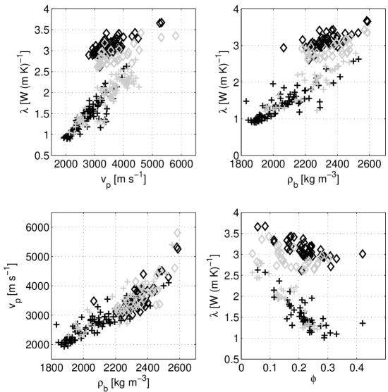
Figure 4: Cross plot of properties measured in the laboratory: Thermal conductivity $\lambda$ versus sonic velocity $v_{p}$ (top left), bulk density $\rho_{b}$ (top right), and porosity $\phi$ (bottom right). $\phi$ is derived from dry and saturated gamma density measurements. Sonic velocity versus bulk density is plotted in the lower left. Black and grey symbols correspond to sandy and carbonaceous samples. Dry and saturated measurements are shown as (+) and ($\diamondsuit$), respectively.

Our goal in measuring the various properties is to predict thermal conductivity from other petrophysical properties which can be measured in-situ. For this purpose we analysed linear correlations between thermal conductivity in dry and saturated condition and and other measurements in their corresponding saturation state. Figure 4 shows cross-plots of these data. Porosity was computed from dry and saturated bulk density. We did not use sonic measurements to compute porosity as velocity-porosity models work best when velocity is measured under confining pressure such that the rock is at its terminal velocity Wyllie1958 ; Mavko1998 . We grouped the samples according to their lithology: The first group contains shaly sandstone samples (“sandy samples”), the second group holds marlstones (“carbonaceous samples”). This division is somewhat preliminary as it is based on geological core descriptions and not on an analysis of the mineral assemblages.

A regression analysis of thermal conductivity versus sonic velocity, bulk density and porosity, respectively, was performed. For each combination a linear equation of the form

$$y=a_{1}x+a_{0}$$ (4)

was fitted to the data. The regression analysis uses a total-least-squares solution to account for measurement errors both in the dependent and independent variables VanHuffel1991 . The Jackknife-method yields the variances of the parameter estimates Shao1995_jackknife . We also computed correlation coefficient $R$ and rms-error to assess the quality of the fit Blobel1998 .

Table 1 summarises the results. If the rms-error is interpreted as the predictive error of the computed relationships it can be deduced that it is possible to calculate thermal conductivity from density and or sonic velocity with an average accuracy of about 0.1–0.2 W(m K)^-1, given an appropriate data set for calibration. Correlation coefficients are largest for dry properties. This is due to the larger contrast in rock and pore volume properties for dry samples. Thus, porosity variations cause larger variations in the effective properties of the two-component system and therefore stronger correlations for dry samples. On the other hand, the low correlation coefficient between thermal conductivity and porosity is due to the complex relationship between these properties. Whereas a linear equation will be sufficient to describe the relationship between thermal conductivity and other petrophysical properties, it is inadequate for porosity. This is addressed in more detail in section 4. Grouping samples according to their lithology has a larger effect on the quality of the fit for saturated than for dry samples. Figure 4 shows in the crossplot of thermal conductivity versus sonic velocity or bulk density that the two lithology groups have the same general trend for dry samples but are separated for saturated measurements. This again is an effect of the strong influence of porosity for dry samples which masks variations due to lithology. From our analysis it thus appears that dry measurements are most sensitive to porosity changes whereas saturated ones reflect both variations in lithology as well as porosity.

The question arises if a correlation using more than one petrophysical property improvea the prediction of thermal conductivity. Table 2 shows the results of a multiple linear regression for thermal conductivity. The equation has the form:

$$\lambda=a_{0}+a_{1}v_{p}+a_{2}\rho+a_{3}\phi$$ (5)

There is only slight improvement over the simple regressions. In practise this improvement might be outweighed by the additional effort for performing the measurements. If the samples are considered to be composed of the three components sand, shale, and carbonate, the quality of the predicted thermal conductivity is directly related to the quality of prediction of these three components from the measured properties. However, quartz and calcite differ in density and velocity by only 3 and 13 %, respectively. Shales have a large variability in their physical properties, but they usually differ considerably from quartz and calcite Ellis1987 ; Crain1986 . Therefore, any of the measurements will be more sensitive to variations of shale content and porosity than to changes in carbonate and sand content. Thus, a combination of sonic velocity and bulk density does not provide significantly more information than each of them alone. This fact can be assessed in a cross-plot of these two properties (Figure 4, lower left panel). Sandy and carbonaceous samples essentially plot on top of each other. Additional measurements, such as natural gamma radiation for instance, are required to characterise our samples better. The contrast in thermal conductivity between quartz and calcite is about 60 %, sufficiently large to separate them in a cross-plot (Figure 4, upper left). This offers opportunities for characterising lithology, as conductivity can be determined rapidly and continuously along a core.

4 Choosing an appropriate mixing law

A mixing law for calculation of the effective thermal conductivity of a composite medium according to the content and thermal conductivity of its components is required both in the analysis of thermal conductivity measured in the laboratory on dry and saturated samples as well as in the prediction of thermal conductivity from logging data. Several models have been proposed and it is instructive to review the relationships most commonly used in geothermics Beardsmore2001 . Effective thermal conductivity $\lambda$ of a layered medium with thermal conductivities $\lambda_{1}$ and $\lambda_{2}$ depends on the direction of the temperature gradient. If heat flow is parallel to the layering the effective conductivity is equal to the arithmetic mean ($\lambda_{a}$) layer thermal conductivities, weighted by their volume fractions. For perpendicular heat flow it corresponds to the harmonic mean ($\lambda_{h}$) Carslaw1959 :

$$\lambda_{a} = V_{1}\lambda_{1}+V_{2}\lambda_{2}$$ (6)

$$\lambda_{h} = \frac{V_{1}}{\lambda_{1}}+\frac{V_{2}}{\lambda_{2}}$$ (7)

While these averages are useful to estimate the average thermal conductivity of a vertical rock sequence they are inappropriate for estimating effective sample thermal conductivities. Narrower bounds can be derived by assuming a geometry where the solid consists of spheres dispersed in the pore fluid or were the fluid is confined in spherical inclusions in the rock matrix Hashin1962 ; Horai1971 . This configurations yield the lower and upper Hashin-Shtrikman (HS^–, HS⁺) bounds, respectively:

$$\lambda_{HS^{-}} = \lambda_{p}+\frac{1-\phi}{\frac{1}{\lambda_{m}-\lambda_{p}}+\frac{\phi}{3\lambda_{p}}}$$ (8)

$$\lambda_{HS^{+}} = \lambda_{m}+\frac{\phi}{\frac{1}{\lambda_{p}-\lambda_{m}}+\frac{\phi}{3\lambda_{m}}}$$ (9)

Here $\phi$ denotes porosity, and the subscripts $p,m$ denote pore and rock matrix properties, respectively. These bounds are of theoretical importance because effective thermal conductivities of rock samples should generally fall in between these bounds. However, in many cases they are to far apart to be of practical use. In this situation an estimate can only be obtained from empirical relationships such as the geometric mean $\lambda_{g}$ Sass1971a , that is often used in geothermal studies:

$$\lambda_{g}=\lambda_{p}^{\phi}\lambda_{m}^{1-\phi}$$ (10)

However, other researcher preferred to use the average of the upper and lower HS bounds Horai1971 , or the square root average $\lambda_{s}$ Roy_1981_thermophysical_properties ; Beardsmore2001 :

$$\sqrt{\lambda_{s}}=\phi\sqrt{\lambda_{p}}+(1-\phi)\sqrt{\lambda_{m}}$$ (11)

The self consistent approach Hill1965 ; Budiansky_1970_composites is popular for elastic properties but is not widely used in geothermal research. For porosities typical for rocks it gives results similar to the square-root average. The thermal conductivity $\lambda_{b}$ for a two component medium is given by the equation:

$$\frac{\phi}{2/3+\lambda_{p}/(3\lambda_{b})}+\frac{1-\phi}{2/3+\lambda_{m}/(3\lambda_{b})}=1$$ (12)

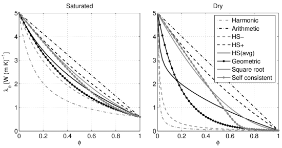
Figure 5: Comparison of different mixing laws for thermal conductivity: HS^$\pm$ - Hashin-Shtrikman upper and lower bounds. HS(avg) - mean of HS⁺ and HS^– bounds. Results are shown for saturated and dry rock samples. Matrix, water, and air thermal conductivities are taken to be 5 W(m K)^-1, 0.6 W(m K)^-1, and 0.026 W(m K)^-1, respectively. Choosing an inappropriate mixing law results in much larger errors for dry samples.

The particular choice of a model becomes important when the contrast in thermal conductivity of the constituents increases. Figure 5 illustrates this by showing bounds and estimates for the saturated and the dry case. Thermal conductivity is assumed to be 5 W(m K)^-1 for the matrix and 0.6 W(m K)^-1 and 0.026 W(m K)^-1 for water and air, respectively. In this case the maximum difference between lower and upper HS bounds are 3.7 and 1.0 W(m K)^-1 for dry and saturated samples. For a two-phase mineral assemblage of crystalline quartz (7.7 W(m K)^-1) and orthoclase (2.3 W(m K)^-1) the maximum difference is as low as 0.4 W(m K)^-1. This shows that the choice of a correct mixing law for a mineral assemblage is somewhat arbitrary while it is essential when considering dry samples. Although a dry sample will rarely occur in nature, these considerations are important when laboratory measurements on dry samples are used to predict in-situ saturated thermal conductivity.

Another important conclusion is, that in the case of a mineral assemblage the geometric mixing law closely follows the lower Hashin-Shtrikman bound, corresponding to a rock model consisting of grains suspended in a fluid. The square root law, on the other hand, is very close to the upper Hashin-Shtrikman bound and could be interpreted as a well lithified rock with spherical pores. Thus, as each particular empirical mixing laws corresponds to a particular rock-structure, one single model cannot be adequate for all different rock structures.

Additional parameters can be introduced in order to incorporate rock structure into a mixing law. Several models assume spheroidal pores where $\alpha$ is the aspect ratio of the spheroids Schulz1981 ; Zimmerman1989 ; Buntebarth1998 ; Popov2003 . In an application of the model by Zimmerman Zimmerman1989 aspect ratios as low as 0.1 were found for basalts Horai1991 , much less than the actual aspect of the pores. It was regarded as a value representing the aspect ratio of the grain contact rather than that of the pores.

From this discussion it appears that mixing laws of varying complexity can be used in different situations: Thermal conductivity of a mineral assemblage or a water-saturated rock can be computed with sufficient accuracy using a geometric mixing law. For measurement on dry samples the pore structure needs to be taken into account. The model proposed in Zimmerman1989 was therefore applied to our laboratory data set in order to determine the aspect ratio $\alpha$. The model assumes a homogeneous mixture of randomly distributed spheroids. For a rock with oblate spheroidal pores one obtains the effective thermal conductivity $\lambda$:

$$\frac{\lambda}{{\lambda_{m}}}=\frac{{(1-\phi)(1-r)+r\beta\phi}}{{(1-\phi)(1-r)+\beta\phi}}$$ (13)

The parameters $\beta$, $M$, and $\theta$ are defined by:

$$r = \frac{{\lambda_{f}}}{{\lambda_{m}}}$$ (14)

$$\beta = \frac{{1-r}}{3}\left({\frac{4}{{2+(r-1)M}}+\frac{1}{{1+(r-1)(1-M)}}}\right)$$ (15)

$$M = \frac{{2\theta-\sin 2\theta}}{{2\tan\theta\sin^{2}\theta}}$$ (16)

$$\theta = \arccos\alpha$$ (17)

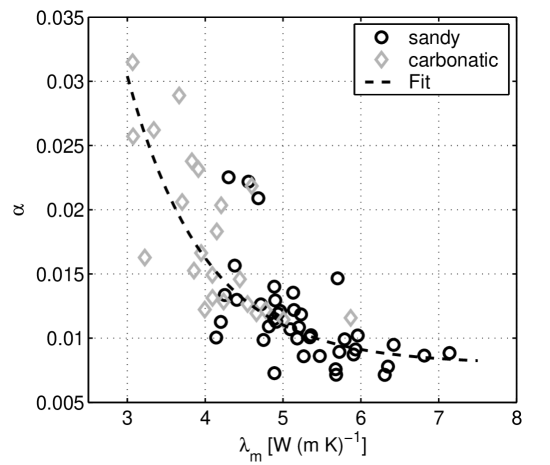
Figure 6: Variation of aspect ratio $\alpha$ versus matrix thermal conductivity $\lambda_{m}$. Both properties are computed using equations 13 and 14. We used dry and saturated thermal conductivity and porosity derived from bulk density as input to the model.

Again, $\alpha$ is the aspect ratio of the spheroidal inclusions. The model described by equations 13 – 17 consists of five parameters: effective, matrix, and pore fluid thermal conductivity, porosity, and aspect ratio. Our measurements of saturated and dry thermal conductivity yield two equations of this type which differ only in the effective thermal conductivity $\lambda$ and the pore fluid thermal conductivity $\lambda_{f}$. This yields seven parameters in total. If we use the two thermal conductivity measurements, known values of water and air thermal conductivity, and an independent porosity measurement, we obtain two equations with two unknowns: Matrix thermal conductivity and pore aspect ratio. We solved the system for our data by a nonlinear iterative algorithm. Figure 6 shows a crossplot of the computed values of matrix thermal conductivity $\lambda_{m}$ and aspect ratio $\alpha$. The median values of $\alpha$ are 0.011 and 0.016 for sandy and carbonaceous samples, respectively. This is about one magnitude less than the values reported in Horai1991 . However, those values were measured on igneous rocks and crack aspect ratios based on sonic or mechanical measurements generally range from 10^-2–10^-3 Cheng1979 ; Zimmerman1984 . Median matrix thermal conductivities are 5.14 W(m K)^-1 and 4.09 W(m K)^-1 for sandy and carbonaceous samples.

5 Thermal conductivity predicted from wireline data

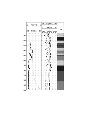
Figure 7: Composite log showing caliper, sonic, neutron porosity, gamma-ray, and core lithology.

Wireline logs of natural gamma radiation (GR), neutron porosity (NPHI), and bulk density (RHOB) were available for analysis in the depth range 570–800 m. In the depth range from 600–800 m caliper (CALI) and temperature (TEMP) had been logged during an aquifer test. The logs are shown together with the core lithology in figure 7. The temperature log is strongly disturbed by water flowing from the formation with temperatures varying from 35–37°C. Unfortunately the disturbance renders a quantitative interpretation of temperatures with regard to the conductive regime impossible. The hole was drilled with 8.5“ diameter and the caliper generally reads below 9“. Some larger diameter sections (630–680 m) are consistent with lithological changes. The core lithology showed no signs of hydrocarbons and the drilled sequence is not known as a hydrocarbon reservoir. Thus, log data quality can be regarded sufficient for quantitative interpretation.

We applied several editing steps before we analysed the logging data. For a general discussion of these steps see for example Jun2002 ; Serra1984 ; Ellis1987 . Logging curves from different tool runs were corrected to common depth points, bad data were eliminated, and environmental corrections applied. Core depths are shifted to match logging depth. Core data are smoothed before they are compared to log curves since these have a lower depth resolution. For this purpose we used an inverse distance algorithm that employs an Gaussian weighting function:

$$w_{k} = \sum_{i=1}^{N}\e^{-\left(\frac{z_{k}-z_{i}}{r_{w}}\right)^{2}}$$ (18)

$$v_{k} = \frac{1}{w_{k}}\sum_{i=1}^{N}v_{i}\e^{-\left(\frac{z_{k}-z_{i}}{r_{w}}\right)^{2}}$$ (19)

Here $v_{k}$ are data values, $z_{i}$ is the depth of the data value, and $w_{k}$ is the normalisation constant. We took the weighting distance $r_{w}$ to be 0.5 m.

In general the response $R^{j}$ of a wireline tool $j$ is determined by the volume fractions $V_{i}$ of the rock components $i$ and their theoretical log response $T_{i}^{j}$. Assuming a linear relationship this results in

$$R^{j}=\sum_{i}V_{i}T_{i}^{j},$$ (20)

with the constraint that $\sum_{i}V_{i}=1$ Doveton1979 ; Hoppie_1996_lithological_characterization . This equation is correct for properties like bulk density or neutron porosity. For acoustic properties, on the other hand, it is not generally valid but results in empirical relationships. If for instance the slowness is considered as the sonic measurement, equation 20 implies Wyllie´s classical travel-time average Wyllie1956 . If the number of constituents equals the number of tool responses equation 20 has one solution. If the number of equations is larger than the number of components, the system is overdetermined and equation 20 can be solved in a least-squares sense. Thus, lithological composition can be computed from a sufficient number of logs. Based on this composition and the known values of thermal conductivity of the components, an effective thermal conductivity can be computed. The geometric average law is used to compute the effective thermal conductivity of the mineral mixture. This value will be used as the matrix thermal conductivity. The effective conductivity of dry and water saturated rocks is then calculated from equation 13 using a median aspect ratio of 0.012. As we want to compare the results to our laboratory data, no temperature correction is necessary at this stage.

As discussed previously for laboratory data, we explore different models with varying simplicity to evaluate how well thermal conductivity can be described by logging data under different circumstances. Two models are of particular interest: (1) One model consists of a mixture of sand, shale, and carbonate and uses the information of all logs available for the borehole; (2) Another model consists only of the two components sand and shale, ignores the carbonate fraction, and uses only wireline logs of slowness and natural gamma radiation, DT and GR, respectively. This model is required for older wells where only these two logs are available. Although these wells have not been logged with modern tools they comprise a large fraction of the available dataset.

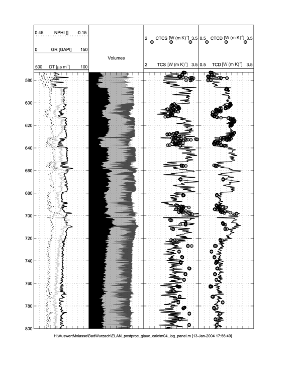
Figure 8: Sand-Shale-Carbonate model for the borehole studied. Input data (left panel): NPHI - neutron porosity; GR - natural gamma radiation; DT - acoustic slowness. Input logs are used to compute the composition (middle left panel). Colour coding: black - shale; light grey - sand; dark grey - carbonates; white - porosity. Composition is then used to compute saturated and dry thermal conductivity, TCS and TCD, respectively (middle right and right panel). Thermal conductivity derived from logs is compared to saturated and dry core data, CTCS and CTCD.

The full model uses logs of gamma density (RHOB), natural gamma radiation (GR), and slowness (DT) as input logs. We employed a commercial software package specialised in deriving rock composition from wireline logs ELANPlus1999 . The three components sand, shale, and carbonate were parameterised in the inversion using response values of the minerals quartz, glauconite, and calcite. The choice of the shale mineral glauconite, an iron-rich variety of illite, is based on the geological description of the cores and general information about the geology of the Upper Freshwater Molasse Geyer1991 . It might not be the only shale mineral present, but the values for illite, another abundant shale mineral, are very similar to the ones we used. Values for the logging properties and mineral thermal conductivities are summarised in Table 3. Thermal conductivity values for quartz and calcite are 7.69 W(m K)^-1 and 3.59 W(m K)^-1, respectively Clauser1995a . The choice for the shale fraction is more difficult. Glauconite was measured with a value of 1.6 W(m K)^-1 Horai1971 . We found that an optimal fit can be obtained with a higher value of 2.2 W(m K)^-1. This discrepancy could be easily explained by the variability of properties for shale minerals, but could also indicate that small amounts of other minerals are present which are not accounted for. There is generally a good agreement between computed and measured thermal conductivity (Figure 8). The rms error of the reconstruction is 0.27 W(m K)^-1 and 0.28 W(m K)^-1 for saturated and dry thermal conductivity. Although the rms-error is slightly larger for dry properties, they can be reproduced much better than saturated properties because the large conductivity contrast of air/rock matrix enhances the variations in thermal conductivity.

The second predictive model employs a simple mineralogy consisting only of sand and shale. Additionally, an empirical relationship is used between sonic velocity $v_{p}$, shale content $V_{Shale}$, and porosity $\phi$, established for shaly sandstones and a pressure range from 10–40 MPa Han1986b . At a pressure of 20 MPa (about 900 m) the equation for the sonic velocity is given by

$$v_{p}\mbox{[km s\textsuperscript{-1}]}=5.49-6.94\phi-2.17V_{Shale}.$$ (21)

The empirical parameters in this equation are slowly varying functions of pressure. For the gamma-ray log we use the linear log response equation 20 assuming no radiation for the fluid:

$$\mbox{GR}=\mbox{GR}_{sand}V_{Sand}+\mbox{GR}_{Shale}V_{Shale}$$ (22)

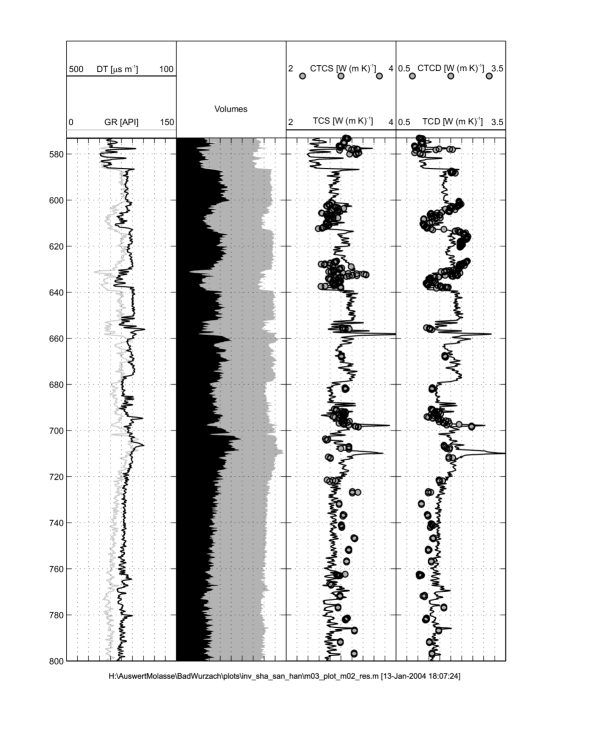
Figure 9: Sand-Shale model for the borehole studied. Input data (left panel): GR - natural gamma radiation; DT - acoustic slowness. Input logs are used to compute the composition (middle left panel). Colour coding: black - shale; light grey - sand; white - porosity. Composition is then used to compute saturated and dry thermal conductivity, TCS and TCD, respectively (middle right and right panel). Thermal conductivity derived from logs is compared to saturated and dry core data, CTCS and CTCD.

The parameters used for the model are given in Table 3. Using the mean density of our laboratory measurements of 2330 kg m^-3, depths were converted to lithostatic pressure which is needed for equation 21. The resulting lithology profile is shown in figure 9.

Again we test this model for its ability to predict thermal conductivities. For this purpose we sampled the compositional log at the depths of the core measurements. Computed composition and measured values of thermal conductivity were then used in an inversion to find optimal mineral thermal conductivities of the constituents (Table 3). A synthetic log of thermal conductivity is then computed and compared to the measurements. The rms-misfit of this two-component model is 0.28 W(m K)^-1, essentially the same as the misfit of the three-component model.

When comparing the lithology logs for the two models it is apparent that the volume fraction of the shale component has not changed very much. The sand fraction of the two-component model also includes the missing carbonate fraction. This is also reflected in the lower mineral thermal conductivity of the sand/shale model. As a consequence the model will be only successful when the ratio of sand and carbonates does not change too much. This can be seen in figure 9 at depths around 630 m, where high thermal conductivities cannot be accurately reproduced by the model.

Both models display a better fit in the upper part of the profile than in the lower part below 700 m. We believe that this is due to an overestimation of porosity for the cores we analysed. Average porosity in the depth range 750–800 m is 20 % for core data but only 17 % for log data. The difference can be attributed to the release of overburden pressure during coring Holt2003_porosity_correction . However, at this point no measurements under confining pressure could be performed to verify this effect. Depending on the geological setting and method to compute an overburden correction, correction factors of 0.85–0.95 have been reported Nieto1994 . It is to be expected that our samples respond strongly to the pressure relief due to their poor consolidation. In this situation log derived porosities might be more accurate and reliable than core derived porosities adding to the usefulness of log derived thermal conductivity.

So far, conductivities were computed only for room temperature. For modeling of temperatures in-situ it is necessary to correct the effect of temperature on thermal conductivity. Temperature dependent thermal conductivity was measured for 23 samples of the Molasse Basin, one of them from the borehole analysed here Clauser2002 . An empirical function based on Sass1992 of the form

$$\lambda(T)=\frac{\lambda_{0}}{a+T(b-c/\lambda_{0})}$$ (23)

was used fit the data Vosteen2003 . Here $\lambda_{0}$ is the thermal conductivity at room temperature (25°C). Coefficients are $a=0.99$, $b=3.4\cdot 10^{-3}$ K^-1, and $c=3.9\cdot 10^{-3}$ W(m K)^-1. Using the aquifer temperature of 36°C at 800 m depth and a range of 2.5–3.5 W(m K)^-1 for saturated thermal conductivity the necessary correction amounts to 5–7 %.

6 Summary and Conclusion

Empirical relationships between thermal conductivity and other petrophysical properties depend on local conditions, in particular the type of diagenesis for the rocks. We analysed core and log data from one borehole in the Molasse Basin in order to establish a set of such equations. Empirical relationships were derived from sonic velocity or bulk density laboratory data that allow to predict thermal conductivity to an accuracy of about 0.2 W(m K)^-1, on average. Predicting thermal conductivity from logging data has a larger error of about 0.3 W(m K)^-1. On the one hand, this may be expected in view of the different spatial resolutions and the problems encountered in the matching of core and log depths. On the other hand, this is outweighed by the larger number of sampling points. An important restriction, as with other studies of this type, is that the results are restricted to the particular conditions in a specific basin.

An ideal combination of wireline logs for an optimum determination of lithology would comprise the full suite of nuclear measurements. In case of the Molasse Basin, we demonstrate that thermal conductivity can be derived even though the number of available logs is less than ideal. This is an important result, as for many old wells - drilled before the advent of modern logging tools - often only a natural gamma log is available. The fact that thermal conductivities can be reconstructed from these data alone makes these older wells attractive for such an analysis.

The discussion of laboratory data and the two compositional models shows that this log combination is most useful in a setting dominated by sand and shale fractions. In contrast, a combination of sandstone and carbonate cannot be well characterised. Fortunately though, these two components differ by a large contrast in thermal conductivity. This measurement can be performed rapidly and yields a continuous profile along the core. Also, thermal conductivity is closely linked to other petrophysical properties, such as permeability Popov2003 . This can be particularly useful, for instance, in reservoir studies where permeability or porosity are important properties.

One aspect which we did not address in our analysis is the variation of thermal conductivity with in situ pressure. Sonic velocity varies strongly with pressure and so does thermal conductivity Clauser1995a ; Seipold1990 . Attempts have been made to model this behaviour with respect to the variation of elastic properties with pressure Sattel1982 ; Zimmerman1989 . Because the Tertiary samples examined in our work are poorly consolidated, a considerable pressure effect may be expected. This requires more detailed study in future.

7 Acknowledgements

Our research was funded by the German Federal Environmental Ministry as part of the activities of its AkEnd Working Group (http://www.akend.de) through Bundesamt für Strahlenschutz (BFS, Federal Agency for Radiation Protection), contract no. 9X0009-8390-0 to RWTH Aachen and contract no. WS 0009-8497-2 to Geophysica Beratungsgesellschaft mbH. We would like to thank the Geological Survey of Baden-Württemberg (LGRB, Freiburg) for providing data and core material. Part of the thermal conductivity measurements were made at the Leibnitz Institute for Applied Geosciences (GGA, Hannover) by H. Deetjen and R. Schellschmidt. Sonic velocity measurements under confining pressure were performed by S. Mayr (TU Berlin). F. Höhne and D. Breuer were responsible for the measurements at RWTH University. The paper was improved by the comments of two anonymous reviewers.

$\lambda$(dry)
Property	Lithology	$a_{1}$	$a_{0}$	$R$	rms
$v_{p}$	all samples	$0.696\pm 0.018$	$-0.485\pm 0.050$	0.921	0.18
$\rho_{b}$	all samples	$2.715\pm 0.086$	$-4.167\pm 0.183$	0.886	0.23
$\phi$	all samples	$-6.289\pm 0.570$	$2.926\pm 0.103$	-0.849	0.24
$v_{p}$	sandy	$0.744\pm 0.028$	$-0.601\pm 0.068$	0.898	0.17
$v_{p}$	carbonate	$0.680\pm 0.031$	$-0.457\pm 0.108$	0.893	0.20
$\rho_{b}$	sandy	$2.500\pm 0.123$	$-3.740\pm 0.250$	0.844	0.22
$\rho_{b}$	carbonate	$2.942\pm 0.179$	$-4.645\pm 0.412$	0.851	0.24
$\phi$	sandy	$-5.783\pm 0.898$	$2.818\pm 0.178$	-0.772	0.25
$\phi$	carbonate	$-6.490\pm 0.489$	$2.939\pm 0.097$	-0.897	0.20
$\lambda$(sat)
$v_{p}$	all samples	$0.378\pm 0.042$	$1.696\pm 0.145$	0.551	0.20
$\rho_{b}$	all samples	$2.214\pm 0.192$	$-2.151\pm 0.452$	0.537	0.23
$\phi$	all samples	$-3.304\pm 0.394$	$3.701\pm 0.083$	-0.363	0.27
$v_{p}$	sandy	$0.372\pm 0.035$	$1.809\pm 0.118$	0.784	0.12
$v_{p}$	carbonate	$0.363\pm 0.056$	$1.537\pm 0.183$	0.449	0.16
$\rho_{b}$	sandy	$2.074\pm 0.263$	$-1.713\pm 0.618$	0.687	0.16
$\rho_{b}$	carbonate	$1.696\pm 0.230$	$-1.112\pm 0.540$	0.548	0.16
$\phi$	sandy	$-3.229\pm 0.541$	$3.828\pm 0.106$	-0.696	0.16
$\phi$	carbonate	$-2.352\pm 0.451$	$3.289\pm 0.101$	-0.331	0.20

Table 1: Results of single regression analysis of thermal conductivity $\lambda$ of core samples based on sonic velocity $v_{p}$, bulk density $\rho_{b}$, and porosity $\phi$. The top panel gives results for dry, the lower part for saturated samples. For each regression the fit parameters $a_{1}$ and $a_{0}$ (Equation 4), with errors, the correlation coefficient $R$, and the rms-error of the fit are shown. Fits were computed both for all samples and grouped by lithology. For ease of display units of $v_{p}$ and $\rho_{b}$ are km s^-1 and g cm^-3, respectively.

Lithology	State	$a_{3}$	$a_{2}$	$a_{1}$	$a_{0}$	rms
sandy	dry	$-0.53\pm 0.14$	$0.615\pm 0.096$	$0.512\pm 0.005$	$-1.14\pm 0.47$	0.15
sandy	sat	$0.042\pm 0.02$	$0.504\pm 0.053$	$0.239\pm 0.002$	$1.07\pm 0.27$	0.12
carbonaceous	dry	$-2.82\pm 0.54$	$0.209\pm 0.031$	$0.371\pm 0.006$	$0.64\pm 1.06$	0.13
carbonaceous	sat	$0.66\pm 0.22$	$1.056\pm 0.172$	$0.100\pm 0.005$	$-0.11\pm 0.83$	0.13
all samples	dry	$-1.19\pm 0.20$	$0.556\pm 0.053$	$0.475\pm 0.002$	$-0.73\pm 0.26$	0.14
all samples	sat	$1.11\pm 0.12$	$0.913\pm 0.076$	$0.243\pm 0.002$	$-0.22\pm 0.38$	0.17

Table 2: Results of the multiple regression of thermal conductivity $\lambda$ versus sonic velocity $v_{p}$, bulk density $\rho_{b}$, and porosity $\phi$ using equation 5. For each regression coefficients of the fit, coefficient error, correlation coefficient $R$, and the rms-error of the fit are given. Fits were computed both for all samples (lower part) and grouped by lithology (upper part). For ease of display units of $v_{p}$ and $\rho_{b}$ are km s^-1 and g cm^-3.

Component		DT	GR	NPHI	$\lambda$
		$\mu$s m-1	API	p.u.	W(m K)-1
Full model
Sand	(quartz)	182	30	-6	7.69
Shale	(glauconite)	295	150	41	2.20
Carbonate	(calcite)	157	11	0	3.59
Sand/shale model
Sand	(quartz)	N/A	30	N/A	6.39
Shale	(glauconite)	N/A	150	N/A	1.96

Table 3: Summary of response parameters and component thermal conductivities used in the log data analysis. Slowness DT, natural gamma radiation GR, and neutron porosity NPHI are used in the complex model. For the simple model NPHI is not used and DT coefficients are determined from equation 21.

References

- (1) C. Clauser, F. Höhne, A. Hartmann, V. Rath, H. Deetjen, W. Rühaak, R. Schellschmidt, A. Zschocke, Erkennen und Quantifizieren von Strömung: Eine geothermische Rasteranalyse zur Klassifizierung des Untergrundes in Deutschland hinsichtlich seiner Eignung zur Endlagerung radioaktiver Stoffe, Endbericht, Department of Applied Geophysics, RWTH Aachen University (2002).
- (2) G. R. Beardsmore, J. P. Cull, Crustal Heat Flow, Cambridge University Press, 2001.
- (3) J. H. Doveton, A. Förster, D. F. Merriam, Predicting thermal conductivity from petrophysical logs: A midcontinent paleozoic case study, in: V. Pawlowsky-Glahn (Ed.), Proceedings of IAMG’97, CIMNE, Barcelona, 1997, pp. 212–217.
- (4) V. Vacquier, Y. Mathieu, E. Legendre, E. Blondin, Experiment on estimating thermal conductivity from oil well logging, American Association of Petroleum Geologists Bulletin 72 (6) (1988) 758–764.
- (5) T. R. Evans, Thermal properties of north sea rocks, Log Analyst 18 (2) (1977) 3–12.
- (6) R. Goss, J. Combs, A. Timur, Prediction of thermal conductivity in rocks from other physical parameters and from standard geophysical well logs, in: Transactions of the SPWLA Annual Logging Symposium, Vol. 16, Society of Professional Well Log Analysts, New Orleans, 1975, p. 21 pp.
- (7) D. D. Blackwell, J. L. Steele, Thermal conductivity of sedimentary rocks: Measurement and significance, in: N. D. Naeser, T. H. McCulloh (Eds.), Thermal History of Sedimentary Basins, Methods and case Histories, Springer, New York, 1989, Ch. 2, pp. 13–35.
- (8) C. F. Williams, A. R., Thermophysical properties of the earth’s crust: In situ measurements from continental and ocean drilling, Journal of Geophysical Research 95 (B6) (1990) 9209–9236.
- (9) F. Brigaud, D. S. Chapman, S. Le Douran, Estimating thermal conductivity in sedimentary basins using lithologic data and geophysical well logs, American Association of Petroleum Geologists Bulletin 74 (9) (1990) 1459–1477.
- (10) L. Demongodin, B. Pinoteau, G. Vasseur, R. Gable, Thermal conductivity and well logs: A case study from the paris basin, Geophysical Journal International 105 (1991) 675–691.
- (11) Y. A. Popov, Optical scanning technology for nondestructive contactless measurements of thermal conductivity and diffusivity of solid matter, in: M. Giot, F. Mayinger , G. P. Celata (Eds.), Experimental Heat Transfer, Fluid Mechanics and Thermodynamics, Proc of the 4th World Congress on Experimental Heat Transfer, Fluid Mechanics and Thermodynamics, Vol. 1, Brussels, Belgium, 1997, pp. 109–116.
- (12) Y. Popov, D. Pribnow, J. Sass, C. Williams, H. Burkhardt, Characterization of rock thermal conductivity by high-resolution optical scanning, Geothermics 28 (2) (1999) 253–276.
- (13) F. Surma, Y. Geraud, Porosity and thermal conductivity of the Soultz-sous-Forets granite, Pure and Applied Geophysics 160 (2003) 1125–1136.
- (14) M. E. Weber, F. Niessen, G. Kuhn, M. Wiedicke, Calibration and application of marine sedimentary physical properties using a multi-sensor core-logger, Marine Geology 136 (1997) 151–172.
- (15) D. V. Ellis, Well logging for earth scientists, Elsevier, Amsterdam, 1987.
- (16) J. R. Hearst, P. H. Nelson, F. L. Paillet, Well logging for physical properties, Wiley, New York, 2000.
- (17) S. Mayr, Der Einfluß der Mikrostruktur auf die Ultraschalleigenschaften von Sandsteinen bei hydrostatischen Druckbedingungen, Ph.D. thesis, Technische Universität Berlin (2002).
- (18) R. W. Zimmerman, W. H. Somerton, M. S. King, Compressibility of porous rocks, Geophysics 91 (B12) (1986) 12765–12777.
- (19) M. R. J. Wyllie, A. R. Gregory, G. H. F. Gardner, An experimental investigation of factors affecting elastic wave velocities in porous media, Geophysics 23 (2) (1958) 459–493.
- (20) G. Mavko, T. Mukerji, J. Dvorkin, The Rock Physics Handbook, Cambridge University Press, Cambridge, U.K., 1998.
- (21) S. V. Huffel, J. Vandewalle, The Total Least Squares Problem: Computational Aspects and Analysis, Vol. 9 of Frontiers in Applied Mathematics, SIAM, Philadelphia, 1991.
- (22) J. Shao, D. Tu, The Jacknife and the Bootstrap, Springer, New York, 1995.
- (23) V. Blobel, E. Lohrmann, Statistische und numerische Methoden der Datenanalyse, B. G. Teubner, Leipzig, 1998.
- (24) E. R. Crain, The Log Analysis Handbook, Volume 1, PennWell, Tulsa, 1986.
- (25) H. S. Carslaw, J. C. Jaeger, Conduction of heat in solids, 2nd Edition, Oxford University Press, 1959.
- (26) Z. Hashin, S. Shtrikman, A variational approach to the theory of the effective magnetic permeability of multiphase materials, Journal of Applied Physics 33 (10) (1962) 3125–3131.
- (27) K.-I. Horai, Thermal conductivity of rock-forming minerals, Journal of Geophysical Research 76 (5) (1971) 1278–1308.
- (28) J. H. Sass, A. H. Lachenbruch, R. J. Munroe, Thermal conductivity of rocks from measurements on fragments and its application to heat-flow determination, Journal of Geophysical Research 76 (14) (1971) 3391–3401.
- (29) R. F. Roy, A. E. Beck, Y. S. Touloukian, Thermophysical properties of rocks, in: Y. S. Touloukian, W. R. Judd, R. F. Roy (Eds.), Physical Properties of Rocks and Minerals, McGraw-Hill, New York, 1981, pp. 409–502.
- (30) R. Hill, A self-consistent mechanics of composite materials, Journal of the Mechanics and Physics of Solids 13 (4) (1965) 213–222.
- (31) B. Budiansky, Thermal and thermoelastic properties of isotropic composites, Journal of Compsite Materials 4 (1970) 286–295.
- (32) B. Schulz, Thermal conductivity of porous and highly porous materials, High Temperatures High Pressures 13 (1981) 649–660.
- (33) R. W. Zimmerman, Thermal conductivity of fluid saturated rocks, Journal of Petroleum Science and Engineering 3 (3) (1989) 219–227.
- (34) G. Buntebarth, J. R. Schopper, Experimental and theoretical investigations on the influence of fluids, solids and interactions between them on thermal properties of porous rocks, Physics and Chemistry of the Earth 23 (9–10) (1998) 1141–1146.
- (35) Y. Popov, V. Tertychnyi, R. Romushkevich, D. Korobkov, J. Pohl, Interrelations between thermal conductivity and other physical properties of rocks: Experimental data, Pure and Applied Geophysics 160 (2003) 1137–1161.
- (36) K.-I. Horai, Thermal conductivity of hawaian basalt: A new interpretation of Robertson and Peck’s data, Journal of Geophysical Research 96 (B3) (1991) 4125–4132.
- (37) C. H. Cheng, M. N. Toksöz, Inversion of seismic velocities for the pore aspect ratio distribution of a rock, Journal of Geophysical Research 84 (B13) (1979) 7533–7543.
- (38) R. W. Zimmerman, The effect of pore structure on the pore and bulk compressibilities of consolidated sandstones, Ph.D. thesis, University of California, Berkeley, Ca. (1984).
- (39) Y. Jun, Reservoir parameters estimation from well log and core data: A case study from the North Sea, Petroleum Geoscience 8 (2002) 63–69.
- (40) O. Serra, Fundamentals of Well-Log Interpretation, Elsevier, New York, 1984.
- (41) J. H. Doveton, H. W. Cable, Fast matrix methods for the lithological interpretation of geophysical logs, Computers & Geology 3 (1979) 101–116.
- (42) B. W. Hoppie, High-resolution lithologic characterization of sequences on the New Jersey margin slope through inversion of leg 150 logging data for lithologies, in: G. S. Mountain, K. G. Miller, P. Blum, C. W. Poag, D. C. Twitchell (Eds.), Proceedings of the Ocean Drilling Program, Scientific Results, Vol. 150, Texas A&M University, College Station, Texas, 1996, pp. 385–409.
- (43) M. R. J. Wyllie, A. R. Gregory, G. H. F. Gardner, Elastic wave velocities in heterogenous and porous media, Geophysics 21 (1956) 41–70.
- (44) Schlumberger, ELANPlus Theory, Austin, TX (1999).
- (45) O. F. Geyer, M. P. Gwinner, Geologie von Baden-Württemberg, 4th Edition, E. Schweizerbart’sche Verlagsbuchhandlung, Stuttgart, Germany, 1991.
- (46) C. Clauser, E. Huenges, Thermal conductivity of rocks and minerals, in: T. J. Ahrens (Ed.), Rock Pysics and Phase Relations – a Handbook of Physical Constants, AGU Reference Shelf, Vol. 3, American Geophysical Union, Washington, 1995, pp. 105–126.
- (47) D. H. Han, A. Nur, D. Morgan, Effects of porosity and clay content on wave velocities in sandstones, Geophysics 51 (1986) 2093–2107.
- (48) R. M. Holt, C. Lehr, C. J. Kentner, P. Spits, In-situ porosity from cores: Poroelastic correction for stress relief during coring, Petrophysics 44 (4) (2003) 253–261.
- (49) J. A. Nieto, D. P. Yale, R. J. Evans, Improved methods for correcting core porosity to reservoir conditions, The Log Analyst 35 (3) (1994) 21–30.
- (50) J. H. Sass, A. H. Lachenbruch, T. H. J. Moses, P. Morgan, Heat flow from a scientific research well at cajon pass, california, Journal of Geophysical Research 97 (B4) (1992) 5017–5030.
- (51) H.-D. Vosteen, R. Schellschmidt, Influence of temperature on thermal conductivity, thermal capacity and thermal diffusivity for different types of rock, Physics and Chemistry of the Earth 28 (9–11) (2003) 499–509.
- (52) U. Seipold, Pressure and temperature dependence of thermal transport properties of granites, High Temperatures High Pressures 22 (1990) 541–548.
- (53) G. Sattel, In situ Bestimmung thermischer Gesteinsparameter aus ihrem Zusammenhang mit Kompressionswellengeschwindigkeit und Dichte, Ph.D. thesis, Universität Karlsruhe, Germany (1982).