A sharp uniform bound for the distribution of sums of Bernoulli trials

Abstract

In this note we establish a uniform bound for the distribution of a sum $S_{n}=X_{1}+\cdots+X_{n}$ of independent non-homogeneous Bernoulli trials. Specifically, we prove that $\sigma_{n}\,\mathbb{P}(S_{n}\!=\!j)\!\leq\!\eta$ where $\sigma_{n}$ denotes the standard deviation of $S_{n}$ and $\eta$ is a universal constant. We compute the best possible constant $\eta\!\sim\!0.4688$ and we show that the bound also holds for limits of sums and differences of Bernoullis, including the Poisson laws which constitute the worst case and attain the bound. We also investigate the optimal bounds for $n$ and $j$ fixed. An application to estimate the rate of convergence of Mann’s fixed point iterations is presented.

Keywords: distribution bounds, sums of Bernoullis, Mann’s iterations

Running title: A sharp uniform bound for sums of Bernoullis

1 Introduction

Let $S_{n}=X_{1}+\cdots+X_{n}$ be a sum of independent non-homogeneous Bernoulli trials with success probabilities $p_{i}$. The distribution of $S_{n}$ is known to be unimodal and bell-shaped with mean $\mu_{n}=\sum_{i=1}^{n}p_{i}$ and variance $\sigma_{n}^{2}=\sum_{i=1}^{n}p_{i}(1\!-\!p_{i})$. Its mode is either $\lfloor\mu_{n}\rfloor$ or $\lceil\mu_{n}\rceil$ or both [8, 25], and the same holds for the median [17]. In this paper we investigate how large it can be the modal probability. More precisely, we establish a uniform upper bound

$$\sigma_{n}\,\mathbb{P}(S_{n}\!\!=\!j)\leq\eta$$ (1)

for all $n$, $j$ and $p_{i}$, and we prove that the best possible constant is

$$\eta=\max_{\lambda\geq 0}\sqrt{2\lambda}\;e^{-2\lambda}\sum_{k=0}^{\infty}\left({\lambda^{k}\over k!}\right)^{2}\sim 0.4688.$$ (2)

The existence of a universal bound (1) can be established using tools related to the local limit theorem [9, 12, 22]. It also follows as a special case of the Kolmogorov-Rogozin concentration inequality [24] which states a more general bound valid for discrete random variables $X_{i}$ with $\sigma_{n}$ replaced by $\sqrt{\sum_{i=1}^{n}(1\!-\!\psi_{i})}$ where $\psi_{i}=\max_{x}\mathbb{P}(X_{i}=x)$. For sums of Bernoullis this is equivalent to (1), so that our contribution is mainly the computation of the optimal constant $\eta$, as well as the identification of the role of the Poisson law in the worst case. Namely, the local limit theorem shows that for a wide range of random variables the limit as $n\to\infty$ in (1) exists and equals $1/\sqrt{2\pi}$. Since $\eta$ exceeds this value, it follows that the worst case situation is not associated with random variables obeying the central limit theorem. It is then natural to expect that the worst case may have to do with the Poisson law, and that is what actually happens. In fact the expression (2) is just

$$\eta=\max_{\lambda\geq 0}\sqrt{2\lambda}\;\mathbb{P}(N_{\lambda}\!=\!N^{\prime}_{\lambda})$$ (3)

where $N_{\lambda}$ and $N^{\prime}_{\lambda}$ are independent Poisson variables with parameter $\lambda$. Since the Poisson law also happens to be extremal in other bounds such as Rosenthal’s inequality (cf. [11, 16, 26, 27]), a natural question is whether (1) might hold for more general sums of random variables.

The inequality (1) complements the large deviation bounds that provide estimates of the form $\mathbb{P}(|S_{n}\!\!-\mathbb{E}(S_{n})|\geq t)\leq f(nt^{2})$ with $f(x)\to 0$ as $x\to\infty$, usually at an exponential rate (cf. [1, 2, 4, 5, 10, 14, 15, 21, 23]). In contrast, (1) does not give such fast asymptotic rates but it can be used to bound $\mathbb{P}(S_{n}\!\!=\!j)$ for all values of $j$ including values close to the mean $\mathbb{E}(S_{n})$. This already proved useful in establishing an optimality guarantee for an approximation algorithm in discrete stochastic optimization (see [6]). In this paper we present another application to the rate of convergence of fixed point iterations for non-expansive maps. In both settings a sharp constant $\eta$ is relevant as it yields better bounds.

The paper is organized as follows. In §2 we show the sharp uniform bound (1) to be valid for all $n,j$ and $p_{i}$’s, and we briefly discuss some extensions to more general distributions including sums and differences of Bernoullis as well as their limits which cover all Poisson distributions and more. In §3 we investigate more closely the optimal bounds for fixed $n$ and $j$. In the final section §4 we show how (1) allows to establish the rate of convergence for fixed point iterations.

2 A sharp uniform bound

Theorem 1

Let $S_{n}\!=\!X_{1}+\cdots+X_{n}$ be a sum of independent Bernoulli trials with $\mathbb{P}(X_{i}\!=\!1)=p_{i}$, and let $\sigma_{n}^{2}\!=\!\sum_{i=1}^{n}p_{i}(1\!-\!p_{i})$ denote its variance. Then

$$\sigma_{n}\;\mathbb{P}(S_{n}\!\!=\!j)\leq\eta$$ (4)

where $\eta=\max_{\lambda>0}\sqrt{2\lambda}\;\mathbb{P}(N_{\lambda}\!=\!N^{\prime}_{\lambda})$ with $N_{\lambda}$ and $N^{\prime}_{\lambda}$ independent Poisson variables of parameter $\lambda$. This bound is sharp and we have more explicitly $\eta=\max_{x\geq 0}\sqrt{x}\,e^{-x}I_{0}(x)\sim 0.4688$, where $I_{0}(x)$ is the modified Bessel function

$$I_{0}(x)=\mbox{$\sum_{k=0}^{\infty}({x^{k}\over 2^{k}k!})^{2}$}=\frac{1}{\pi}\int_{0}^{\pi}\!\!\exp(x\cos\theta)\,d\theta.$$

Proof. Consider the generating function $\phi(z)=\mathbb{E}(z^{S_{n}})=\sum_{j=0}^{n}\mathbb{P}(S_{n}\!=\!j)z^{j}$. Integrating $\phi(z)/z^{j+1}$ along the unit circle $\mathcal{C}$ in the complex plane we get

$$\mathbb{P}(S_{n}\!=\!j)=\mbox{${1\over 2\pi i}\int_{\mathcal{C}}{\phi(z)\over z^{j+1}}\,dz={1\over 2\pi}\int_{0}^{2\pi}\!\phi(e^{i\theta})e^{-ij\theta}\,d\theta$}$$ (5)

so that taking absolute value it follows that

$$\mathbb{P}(S_{n}\!=\!j)\leq\mbox{${1\over 2\pi}\int_{0}^{2\pi}\!|\phi(e^{i\theta})|\,d\theta$}.$$ (6)

The independence of the $X_{i}$’s yields $\phi(z)=\mathbb{E}[\prod_{i=1}^{n}z^{X_{i}}]=\prod_{i=1}^{n}[(1\!-\!p_{i})+p_{i}z]$, from which we obtain

$$|\phi(e^{i\theta})|=\prod_{i=1}^{n}\sqrt{1+2p_{i}(1\!-\!p_{i})(\cos\theta\!-\!1)}.$$

Using the inequality $1+y_{i}\leq\exp(y_{i})$ with $y_{i}=2p_{i}(1\!-\!p_{i})(\cos\theta\!-\!1)$, and setting $x=\sum_{i=1}^{n}p_{i}(1\!-\!p_{i})$, we deduce

$$|\phi(e^{i\theta})|\leq\prod_{i=1}^{n}\exp(y_{i}/2)=\exp(x(\cos\theta\!-\!1)),$$

and since $\sigma_{n}=\sqrt{x}$ we conclude

$$\sigma_{n}\,\mathbb{P}(S_{n}=j)\leq\sqrt{x}\mbox{$\frac{1}{2\pi}\int_{0}^{2\pi}\exp(x(\cos\theta\!-\!1))\,d\theta$}=\sqrt{x}\,e^{-x}I_{0}(x)\leq\eta.$$

In order to show that the bound is sharp, consider a sum of $n=2a$ Bernoullis, half of them with $p_{i}=\lambda/a$ and the other half with $p_{i}=1\!-\!\lambda/a$, so that $S_{n}=U+V$ with $U\sim B(a,\lambda/a)$ and $V\sim B(a,1\!-\!\lambda/a)$ independent Binomials. Note that $V\stackrel{{\scriptstyle d}}{{=}}a-U^{\prime}$ with $U^{\prime}$ an independent copy of $U$, and for $j=a$ we get

$$\sigma_{n}\,\mathbb{P}(S_{n}\!=\!a)=\mbox{$\sqrt{2\lambda(1\!-\!{\lambda\over a})}\;\mathbb{P}(U=U^{\prime}).$}$$

Since $U$ and $U^{\prime}$ converge as $a\to\infty$ to independent Poisson variables $N_{\lambda}$ and $N^{\prime}_{\lambda}$ with parameter $\lambda$, this expression tends to

$$\sqrt{2\lambda}\;\mathbb{P}(N_{\lambda}=N^{\prime}_{\lambda})=\sqrt{2\lambda}\,e^{-2\lambda}\sum_{k=0}^{\infty}(\mbox{${\lambda^{k}\over k!}$})^{2}=\sqrt{2\lambda}\,e^{-2\lambda}I_{0}(2\lambda)$$

which proves that the bound is sharp.

Remark 1. The optimal bound $\eta=\max_{\lambda>0}\sqrt{2\lambda}\;\mathbb{P}(N_{\lambda}\!=\!N^{\prime}_{\lambda})$ is approximately $\eta\sim 0.468822355499$ which is attained for $\lambda\sim 0.39498893$.

Remark 2. The proof above shows that the bound $\eta$ is asymptotically attained for a sum of two Binomials with different success probabilities $p=\lambda/a$ and $p^{\prime}=1-\lambda/a$. As a matter of fact, allowing for two different Binomials is essential since for a single Binomial $S_{n}\sim B(n,x)$ we have the sharper bound

$$\sigma_{n}\,\mathbb{P}(S_{n}\!=\!j)=\mbox{$\sqrt{n\,x(1\!-\!x)}\;{n\choose j}x^{j}(1\!-\!x)^{n-j}\leq{1\over\sqrt{2e}}$}$$ (7)

with ${1\over\sqrt{2e}}\sim 0.4289<\eta$. To prove (7) we note that for $n$ and $j$ given, the maximum over $x\in[0,1]$ is attained at $x=(j+{1\over 2})/(n+1)$, so that replacing this value all we must show is that $C^{n}_{j}\leq{1\over\sqrt{2e}}$ where

$$C^{n}_{j}={n\choose j}{\sqrt{n}(j+\mbox{${1\over 2}$})^{j+{1\over 2}}(n-j+\mbox{${1\over 2}$})^{n-j+{1\over 2}}\over(n+1)^{n+1}}.$$

Now $C^{n}_{j+1}/C^{n}_{j}=H(n-j)/H(j+1)$ where $H(x)=x(x-\mbox{${1\over 2}$})^{x-\mbox{${1\over 2}$}}/(x+\mbox{${1\over 2}$})^{x+\mbox{${1\over 2}$}}$ is decreasing, so that $C^{n}_{j}$ decreases for $j\leq{n-1\over 2}$ and increases afterwards. Hence $C_{j}^{n}$ is maximal at $j=0$ or $j=n$, and then the conclusion follows since

$$C^{n}_{0}=C^{n}_{n}={1\over\sqrt{2}}\sqrt{n\over n+{1\over 2}}\left(1-{1\over 2(n+1)}\right)^{n+1}\leq{1\over\sqrt{2}}\exp(-\mbox{${1\over 2}$})={1\over\sqrt{2e}}.$$

2.1 Extension to more general distributions

As a consequence of Theorem 1 we see that (1) still holds for any random variable $S_{n}\!=\!\sum_{i=1}^{n}\pm X_{i}$ that can be expressed as sums and differences of independent Bernoullis. Moreover, the bound remains true for limits of such variables, which includes all Poisson distributions as well as infinite series $S^{\infty}=\sum_{i=1}^{\infty}X_{i}$ of independent Bernoullis with $\sum_{i=1}^{\infty}p_{i}<\infty$, namely

Corollary 2

Let $S=(X+S^{\infty}_{+})-(Y+S^{\infty}_{-})$ with $X,Y$ independent Poisson and $S^{\infty}_{+},S^{\infty}_{-}$ convergent series of independent Bernoullis. Then for all $j\in\mathbb{Z}$ we have $\sigma_{S}\,\mathbb{P}(S\!=\!j)\leq\eta$.

A natural question is whether such uniform bounds hold for more general distributions. In particular it would be interesting to characterize the distributions that can be obtained as limits of sums and differences of Bernoullis, beyond those in Corollary 2. In this respect we recall the fundamental result of Kintchine [18] (see also Gnedenko and Kolmogorov [13, Theorem 2, p.115]) which characterizes the limit distributions for sums of independent variables. The latter may or may not be Bernoullis, so that this general result provides only necessary conditions for our more specific question.

Remark 3. Following Remark 2, in the case of a simple Binomial $S\sim B(n,x)$, as well as for a single Poisson $S\sim\mathcal{P}(\lambda)$, which is a limit of Binomials $B(n,{\lambda\over n})$, we have the stronger bound $\sigma_{S}\,\mathbb{P}(S\!=\!j)\leq{1\over\sqrt{2e}}$.

3 Optimal bounds for fixed $n$ and $j$

Let us consider next the bound (1) for $n$ and $j$ fixed, namely

$$V_{j}^{n}=\max_{p\in[0,1]^{n}}R_{j}^{n}({}p)$$

where $R^{n}_{j}(p)=\sigma_{n}P^{n}_{j}$ with $\sigma_{n}\!=\!\sqrt{\sum_{i=1}^{n}p_{i}(1\!-\!p_{i})}$ and

$$P^{n}_{j}=\mathbb{P}(S_{n}\!=\!j)=\sum_{|A|=j}\mbox{$\prod_{i\in A}p_{i}\cdot\prod_{i\not\in A}(1\!-\!p_{i}).$}$$

Clearly the maximum $V_{j}^{n}$ is attained and, since $R^{n}_{j}(p)$ is symmetric, any permutation of an optimal solution remains optimal. Moreover, replacing each $p_{i}$ by $(1\!-\!p_{i})$ we have the symmetry $V^{n}_{n-j}=V^{n}_{j}$. It is also clear that $V^{n}_{j}$ increases with $n$ since when computing $V^{n+1}_{j}$ one may always take $p_{n+1}=0$. More generally, for $n<m$, by appropriately choosing $p_{i}\in\{0,1\}$ for $n<i\leq m$, we get

$$V^{n}_{j}\leq V_{k}^{m}\quad\forall k=j,\ldots,j+(m-n),$$ (8)

and in particular

$$V_{j}^{n}\leq V_{n}^{2n}.$$ (9)

This shows that $V^{n}_{j}$ is dominated by $V^{2n}_{n}$ so that the optimal uniform bound in (1) is attained as an increasing limit

$$\eta=\lim_{a\to\infty}V^{2a}_{a}.$$

While this was already noted in the proof of Theorem 1, the inequalities above give a more precise picture. As a matter of fact, from (8) it follows that for $n$ large, all but a small fraction of the $V^{n}_{j}$’s will be near $\eta$. More precisely,

Proposition 3

For each $\varepsilon>0$ there exists $n_{0}\in\mathbb{N}$ such that for $n\geq n_{0}$ and all $j$ with $\varepsilon n\leq j\leq(1-\varepsilon)n$ we have $\eta-\varepsilon\leq V^{n}_{j}\leq\eta$.

Proof. Let us fix $\varepsilon>0$ and for each $n$ take $a=\lfloor\varepsilon n\rfloor$. For $j$ as in the statement we have $a\leq j\leq n-a$ and we may use (8) to get $V^{2a}_{a}\leq V^{n}_{j}$. It suffices then to choose $n$ large so that $a$ is also large enough to ensure $V^{2a}_{a}>\eta-\varepsilon$.

Remark 4. The previous result does not hold uniformly for all $j$. In fact, for $j=0$ one explicitly finds the optimum $p_{1}=\ldots=p_{n}=\frac{1}{2(n+1)}$ so that

$$V_{0}^{n}=V_{n}^{n}=\mbox{$\sqrt{\frac{n}{2n+1}}$}\left(1-\mbox{$\frac{1}{2(n+1)}$}\right)^{n+1}$$

which converges as $n\to\infty$ towards $\frac{1}{\sqrt{2e}}$ which is strictly smaller than $\eta$.
Conjecture 1. Numerical computations suggest that $V^{n}_{j}$ increases with $j$ for $j\leq\frac{n}{2}$ and decreases afterwards. Moreover, $V^{n}_{j}$ seems to be concave in $j$.

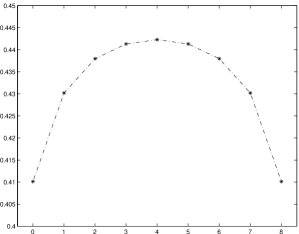
Figure 1: Profile of $V^{n}_{j}$ for $j=0,\ldots,n$ (here $n=8$)

3.1 Reduction to a sum of 2 Binomials

We show next that when computing the maximum $V^{n}_{j}$ we may restrict to $p_{i}$’s that take only two distinct values. This fact was established in [28, Vaisman] but has not been published elsewhere. Let us first prove that the maximum $V_{j}^{n}$ is attained with $0<p_{i}<1$ for all $i=1,\ldots,n$, which is equivalent to showing that the inequalities (8) are strict. We exploit the following properties.

Lemma 4

Let $p$ be optimal for $V^{n}_{j}$ and let $P^{n}_{k}=\mathbb{P}(S_{n}=k)$ be the corresponding distribution with mean $\mu_{n}$ and variance $\sigma_{n}^{2}$. If $0<p_{i}<1$ for $i=1,\ldots,n$ then

• $2\sigma_{n}^{2}[P^{n}_{j}-P^{n}_{j+1}]=\frac{\mu_{n}}{j+1}P^{n}_{j}$,

• $2\sigma_{n}^{2}[P^{n}_{j}-P^{n}_{j-1}]=\frac{n-\mu_{n}}{n-j+1}P^{n}_{j}$,

• $S_{n}$ has a unique mode at $j$,

• $\sigma_{n}^{2}[j-\mu_{n}]+\sum_{i=1}^{n}p_{i}(1\!-\!p_{i})(\mbox{$\frac{1}{2}$}-p_{i})=0$,

• $j-\frac{1}{2}<\mu_{n}<j+\frac{1}{2}$.

Proof. Letting $S^{i}=\sum_{j\neq i}X_{j}$ and $Q_{k}^{i}=\mathbb{P}(S^{i}\!=\!k)$ we have the known identities

$$P^{n}_{k} = p_{i}Q^{i}_{k-1}+(1\!-\!p_{i})Q_{k}^{i},$$ (10)

$$kP^{n}_{k} = \sum_{i=1}^{n}p_{i}Q^{i}_{k-1}.$$ (11)

Since $p$ is an interior optimal solution, the optimality conditions give

$$\frac{\partial R_{j}^{n}}{\partial p_{i}}=\frac{1-2p_{i}}{2\sigma_{n}}P^{n}_{j}+\sigma_{n}[Q^{i}_{j-1}-Q^{i}_{j}]=0$$ (12)

which multiplied by $p_{i}/\sigma_{n}$ and summed over $i$ yields

$$\mbox{$\frac{1}{2\sigma_{n}^{2}}$}P^{n}_{j}\sum_{i=1}^{n}p_{i}(1\!-\!2p_{i})+\sum_{i=1}^{n}p_{i}[Q^{i}_{j-1}-Q^{i}_{j}]=0.$$

The first sum is just $2\sigma_{n}^{2}-\mu_{n}$, while (11) shows that the second sum is equal to $jP^{n}_{j}-(j+1)P^{n}_{j+1}$, so that rearranging terms we get (a).

Property (b) follows from (a) applied to $\bar{p}_{i}=1\!-\!p_{i}$ which is optimal for $V^{n}_{n-j}$, while (c) is a consequence of the fact that the distribution of $S_{n}$ is unimodal combined with (a) and (b) that give respectively $P^{n}_{j}>P_{j+1}^{n}$ and $P^{n}_{j}>P^{n}_{j-1}$.

To prove (d) we multiply (12) by $\sigma_{n}\,p_{i}(1\!-\!p_{i})$ and sum over $i$ to get

$$P^{n}_{j}\sum_{i=1}^{n}p_{i}(1\!-\!p_{i})(\mbox{$\frac{1}{2}$}-p_{i})+\sigma_{n}^{2}\sum_{i=1}^{n}p_{i}(1\!-\!p_{i})[Q^{i}_{j-1}-Q^{i}_{j}]=0.$$ (13)

Now, from (10) we have $P^{n}_{j}-Q^{i}_{j-1}=(1\!-\!p_{i})[Q^{i}_{j}-Q^{i}_{j-1}]$ and using (11) we get

$$\sum_{i=1}^{n}p_{i}(1\!-\!p_{i})[Q^{i}_{j-1}-Q^{i}_{j}]=\sum_{i=1}^{n}p_{i}[Q^{i}_{j-1}-P^{n}_{j}]=[\mbox{$j-\sum_{i=1}^{n}p_{i}$}]P^{n}_{j}$$

which plugged into (13) and simplifying by $P^{n}_{j}$ yields (d).

Finally, to prove (e) it suffices to observe that (d) can be rewritten as

$$\sigma_{n}^{2}[\mbox{$j+\frac{1}{2}-\mu_{n}$}] = \hskip 7.3194pt\mbox{$\sum_{i=1}^{n}p_{i}^{2}(1\!-\!p_{i})$}~{}>0,$$

$$\sigma_{n}^{2}[\mbox{$j-\frac{1}{2}-\mu_{n}$}] = -\mbox{$\sum_{i=1}^{n}p_{i}(1\!-\!p_{i})^{2}$}<0.$$

Proposition 5

If $p$ attains the maximum $V_{j}^{n}$ then $0<p_{i}<1$ for $i=1,\ldots,n$. Moreover, for $n<m$ all the inequalities (8) are strict.

Proof. The strict inequality in (8) is a direct consequence of the fact that the optimal $p_{i}$’s do not take the values 0 nor 1. We prove the latter by induction in $n$. The property clearly holds for $n=1$. Assume that it holds for a given $n$ and let us prove it for $n+1$. Take $p$ optimal for $V^{n+1}_{j}$ and suppose for a contradiction that it has a null component, say $p_{n+1}=0$. In this case $V^{n+1}_{j}=V^{n}_{j}$ and $(p_{1},\ldots,p_{n})$ is optimal for $V_{j}^{n}$ so the induction hypothesis yields $0<p_{i}<1$ for $i=1,\ldots,n$. Denoting as before $P^{n}_{k}=\mathbb{P}(S_{n}=k)$ and using properties (b) and (e) in Lemma 4 we obtain

$$\frac{\partial R^{n+1}_{j}}{\partial p_{n+1}}=\frac{1}{2\sigma_{n}}P^{n}_{j}+\sigma_{n}[P^{n}_{j-1}-P^{n}_{j}]=\frac{P^{n}_{j}}{2\sigma_{n}}\frac{\mu_{n}-j+1}{n-j+1}>0$$

which shows that $p_{n+1}=0$ cannot be a maximizer. This same argument applied to $\bar{p}_{i}=1\!-\!p_{i}$, which is optimal for $V^{n+1}_{n-j}$, shows that no $p_{i}$ can be equal to 1.

With this result we may now show that when computing $V^{n}_{j}$ one may restrict to a sum of two Binomials.

Proposition 6

There exists $p$ optimal for $V^{n}_{j}$ which takes at most two distinct values $p_{i}\in\{\alpha,\beta\}$ with $\alpha,\beta\in(0,1)$. In other words, the maximum is attained for $S_{n}=U+V$ with $U\sim B(a,\alpha)$ and $V\sim B(b,\beta)$ independent Binomials with $a+b=n$. More explicitly, denoting $b^{n}_{k}(x)={n\choose k}x^{k}(1\!-\!x)^{n-k}$, we have

$$V^{n}_{j}=\max_{\stackrel{{\scriptstyle\mbox{\scriptsize$a\!+\!b=n$}}}{{\alpha,\beta\in(0,1)}}}\sqrt{a\,\alpha(1\!-\!\alpha)+b\,\beta(1\!-\!\beta)}\;\sum_{k=0}^{j}b^{a}_{k}(\alpha)b^{b}_{j-k}(\beta).$$ (14)

Proof. Take $p$ an optimal solution for $V^{n}_{j}$ with the smallest product $\Pi_{i=1}^{n}p_{i}$. We claim that this $p$ takes at most two values. Assume by contradiction that it has 3 different entries $0\!<\!p_{r}\!<\!p_{s}\!<\!p_{t}\!<\!1$. Denoting $\tilde{p}=(p_{i})_{i\neq r,s,t}$ and $\bar{p}_{i}=1-p_{i}$ we have

$$P^{n}_{j} = p_{r}p_{s}p_{t}P^{n-3}_{j-3}(\tilde{p})+[\bar{p}_{r}p_{s}p_{t}+p_{r}\bar{p}_{s}p_{t}+p_{r}p_{s}\bar{p}_{t}]P^{n-3}_{j-2}(\tilde{p})$$

$$\mbox{}+[\bar{p}_{r}\bar{p}_{s}p_{t}+\bar{p}_{r}p_{s}\bar{p}_{t}+p_{r}\bar{p}_{s}\bar{p}_{t}]P^{n-3}_{j-1}(\tilde{p})+\bar{p}_{r}\bar{p}_{s}\bar{p}_{t}P^{n-3}_{j}(\tilde{p})$$

which may be rewritten as $P^{n}_{j}=F(p_{r},p_{s},p_{t})$ where

$$F(x,y,z)=Axyz+B(xy\!+\!xz\!+\!yz)+C(x\!+\!y\!+\!z)+D$$

with coefficients $A,B,C,D$ that depend only on $\tilde{p}$. Setting $\kappa=P^{n}_{j}/2\sigma_{n}^{2}$ the optimality conditions for $p$ yield

$$\kappa(1\!-\!2p_{r})+Ap_{s}p_{t}+B(p_{s}+p_{t})+C = 0$$

$$\kappa(1\!-\!2p_{s})+Ap_{r}p_{t}+B(p_{r}+p_{t})+C = 0$$

$$\kappa(1\!-\!2p_{t})+Ap_{r}p_{s}+B(p_{r}+p_{s})+C = 0.$$

Substracting the first two equations and simplifying by $p_{s}-p_{r}\neq 0$ we get $2\kappa+Ap_{t}+B=0$, while the second and third equations give $2\kappa+Ap_{r}+B=0$. Hence $Ap_{t}=Ap_{r}$ and since $p_{r}\neq p_{t}$ we conclude $A=0$ so that $F(x,y,z)$ depends only on $x+y+z$ and $xy+xz+yz$. Moreover, since we also have

$$x(1\!-\!x)+y(1\!-\!y)+z(1\!-\!z)=(x\!+\!y\!+\!z)-(x\!+\!y\!+\!z)^{2}+2(xy\!+\!xz\!+\!yz)$$

it follows that $R^{n}_{j}(x,y,z,\tilde{p})$ is constant over the set defined by the equations $x\!+\!y\!+\!z=p_{r}\!+\!p_{s}\!+\!p_{t}$ and $xy\!+\!xz\!+\!yz=p_{r}p_{s}\!+\!p_{r}p_{t}\!+\!p_{s}p_{t}$. Thus, any such vector $(x,y,z,\tilde{p})$ maximizes $R^{n}_{j}(\cdot)$ and our choice of $p$ implies that $(p_{r},p_{s},p_{t})$ solves

$$\left\{\begin{array}[]{l}\min~{}~{}xyz\\ s.t.~{}~{}(x,y,z)\in[0,1]^{3}\\ \begin{array}[]{lcl}x+y+z&=&p_{r}+p_{s}+p_{t}\\ xy+xz+yz&=&p_{r}p_{s}+p_{r}p_{t}+p_{s}p_{t}.\end{array}\end{array}\right.$$

Since $p_{r},p_{s},p_{t}$ are different, the gradients of the two equality constraints at this optimal point are linearly independent, while the inequality constraints are non-binding. Hence the Mangasarian-Fromovitz constraint qualification holds and we may find Lagrange multipliers $\lambda$ and $\mu$ such that

$$p_{s}p_{t} = \lambda+\mu(p_{s}+p_{t})$$

$$p_{r}p_{t} = \lambda+\mu(p_{r}+p_{t})$$

$$p_{r}p_{s} = \lambda+\mu(p_{r}+p_{s}).$$

Substracting the first two equations and simplifying by $p_{s}\!-p_{r}\!\neq\!0$ we get $p_{t}\!=\!\mu$, and similarly $p_{r}=\mu$ and $p_{s}=\mu$. This contradiction shows that $A$ cannot be 0, and therefore the assumption $0<p_{r}<p_{s}<p_{t}<1$ was absurd.

Conjecture 2: We conjecture that for each $n$ and $j$ there exist unique values $\alpha<\frac{1}{2}<\beta$ such that the maximizers of $V^{n}_{j}$ are precisely the vectors with exactly $(n-j)$ components equal to $\alpha$ and $j$ components equal to $\beta$.

Remark 4 shows that this property holds for $V^{n}_{0}$ and $V^{n}_{n}$. In the next section we prove that it also holds for the dominating values $V^{2a}_{a}$ and, moreover, in this case $\alpha+\beta=1$.

3.2 Computation of the sharp bound $V^{2a}_{a}$

Proceeding as in the proof of Theorem 1, setting $z_{i}=p_{i}(1\!-\!p_{i})\in[0,\frac{1}{4}]$ we have

$$\mathbb{P}(S_{n}=j)\leq\frac{1}{2\pi}\int_{0}^{2\pi}\prod_{i=1}^{n}\sqrt{1+2z_{i}(\cos\theta-1)}\;d\theta$$

so that using the change of variables $\theta=2\xi$ we get

$$R^{n}_{j}({}p)\leq\Phi_{n}(z):=\sqrt{\mbox{$\sum_{i=1}^{n}z_{i}$}}\int_{0}^{\pi}\!\!\frac{1}{\pi}\prod_{i=1}^{n}\sqrt{1\!-\!4z_{i}\sin^{2}\!\xi}\;d\xi.$$ (15)

Therefore, denoting $\eta_{n}$ the maximum of $\Phi_{n}(z)$ for $z\in[0,\frac{1}{4}]^{n}$ we have $V^{n}_{j}\leq\eta_{n}$. We will prove that for $n=2a$ and $j=a$ we have the equality $V^{2a}_{a}=\eta_{2a}$. Moreover, we will show that $V^{2a}_{a}$ has a unique maximizer $p$ up to permutation. We begin by characterizing the maximum of $\Phi_{n}$ for $n=2a$.

Lemma 7

For $n=2a$ the map $\Phi_{n}(z)$ has a unique maximizer $z\in[0,\frac{1}{4}]^{n}$ which is of the form $z_{i}=\bar{z}$ for all $i=1,\ldots,n$ with $\bar{z}\in(0,\frac{1}{4})$.

Proof. Let $z\in[0,\frac{1}{4}]^{n}$ maximize $\Phi_{n}$. Denoting $Q_{z}(\xi)=\frac{1}{\pi}\prod_{i=1}^{n}\sqrt{1\!-\!4z_{i}\sin^{2}\!\xi}$ and $s=\sum_{i=1}^{n}z_{i}$ we have

$$\frac{\partial\Phi_{n}}{\partial z_{k}}(z)=\frac{1}{2\sqrt{s}}\int_{0}^{\pi}\!\!\!Q_{z}(\xi)d\xi-2\sqrt{s}\int_{0}^{\pi}\!\!\!Q_{z}(\xi)\frac{\sin^{2}\!\xi}{1\!-\!4z_{k}\sin^{2}\!\xi}d\xi.$$ (16)

Clearly the $z_{i}$’s are not all 0. They cannot be all equal to $\frac{1}{4}$ either, since in that case we would have $Q_{z}(\xi)=\frac{1}{\pi}\cos^{2a}\!\xi$ so that letting

$$J^{k,i}=\frac{1}{\pi}\int_{0}^{\pi}\cos^{2k}\!\xi\sin^{2i}\!\xi\,d\xi=\frac{1}{4^{k+i}}\frac{(2k)!(2i)!}{k!i!(k+i)!}$$

we get the following inequality that contradicts optimality

$$\frac{\partial\Phi_{n}}{\partial z_{k}}(z)=\mbox{$\frac{1}{\sqrt{2a}}$}\,J^{a,0}-\sqrt{2a}\,J^{a-1,1}=-\mbox{$\sqrt{2a}\,\frac{(2a-2)!}{(2^{a}a!)^{2}}$}<0.$$

Hence, there is some component $z_{k}\in(0,\frac{1}{4})$ for which we have $\frac{\partial\Phi_{n}}{\partial z_{k}}=0$. Using (16) we then get $\frac{\partial\Phi_{n}}{\partial z_{i}}=\frac{\partial\Phi_{n}}{\partial z_{i}}-\frac{\partial\Phi_{n}}{\partial z_{k}}=(z_{k}-z_{i})Q_{ik}$ with

$$Q_{ik}=\int_{0}^{\pi}\!\!\!\frac{8\sqrt{s}\,Q_{z}(\xi)\sin^{4}\!\xi}{[1\!-\!4z_{k}\sin^{2}\!\xi][1\!-\!4z_{i}\sin^{2}\!\xi]}d\xi.$$

Note that if $z_{i}=\frac{1}{4}$ and all the other components are smaller than $\frac{1}{4}$ this integral is singular and $Q_{ik}=\infty$. In all other cases $Q_{ik}$ is finite and strictly positive. Hence, if $z_{i}=0$ we get $\frac{\partial\Phi_{n}}{\partial z_{i}}>0$ contradicting optimality, while $z_{i}=\frac{1}{4}$ leads to the contradiction $\frac{\partial\Phi_{n}}{\partial z_{i}}<0$. Therefore $z_{i}\in(0,\frac{1}{4})$ so that $\frac{\partial\Phi_{n}}{\partial z_{i}}=0$, which implies $z_{i}=z_{k}$ and then $z=(\bar{z},\ldots,\bar{z})$ with $\bar{z}\in(0,\frac{1}{4})$.

It remains to show that $\bar{z}$ is unique. A routine calculation shows that the optimality condition $\frac{\partial\Phi_{n}}{\partial z_{k}}(\bar{z},\ldots,\bar{z})=0$ is equivalent to $h(\bar{z})=0$ where $h(z)$ is the polynomial

$$h(z)=\frac{2a\!+\!1}{\pi}\int_{0}^{\pi}\!\![1\!-\!4z\sin^{2}\!\xi]^{a}d\xi-\frac{2a}{\pi}\int_{0}^{\pi}\!\![1\!-\!4z\sin^{2}\!\xi]^{a-1}d\xi.$$

According to Fourier-Budan’s Theorem the number of roots in $(0,\frac{1}{4})$ is at most $\sigma(0)-\sigma(\frac{1}{4})$ where $\sigma(z)$ denotes the number of sign changes in the sequence $h(z),h^{\prime}(z),h^{\prime\prime}(z),\ldots,h^{(a)}(z)$. By direct calculation we get

$$h^{(i)}(z)=\frac{(-4)^{i}a!}{(a-i)!}\frac{1}{\pi}\int_{0}^{\pi}[1-4z\sin^{2}\!\xi]^{a-i}\sin^{2i}\!\xi\left[2a+1-\frac{2(a-i)}{1\!-\!4z\sin^{2}\!\xi}\right]d\xi.$$

Hence $h^{(i)}(0)=\frac{(-4)^{i}a!}{(a-i)!}(2i+1)J^{0,i}$ which alternates sign so that $\sigma(0)=a$. Also

$$h^{(i)}(\mbox{$\frac{1}{4}$}) = \frac{(-4)^{i}a!}{(a-i)!}\frac{1}{\pi}\int_{0}^{\pi}\cos^{2(a-i)}\!\xi\sin^{2i}\!\xi\left[2a+1-\frac{2(a-i)}{\cos^{2}\!\xi}\right]d\xi$$

$$= \frac{(-4)^{i}a!}{(a-i)!}\left[(2a\!+\!1)J^{a-i,i}-2(a\!-\!i)J^{a-i-1,i}\right]$$

where for $i=a$ the last term $J^{-1,a}$ is interpreted as 0. Explicitely we get

$$h^{(i)}(\mbox{$\frac{1}{4}$})=\left\{\begin{array}[]{ll}(-1)^{i+1}4^{i-a}\frac{(2a-2i)!(2i)!}{(a-i)!^{2}i!}\frac{2i+1}{2a-2i-1}&\mbox{ for $i<a$}\\[4.30554pt] (-1)^{a}(2a\!+\!1)\frac{(2a)!}{a!}&\mbox{ for $i=a$}\end{array}\right.$$

which yields $\sigma(\frac{1}{4})=a-1$. Hence $\sigma(0)-\sigma(\frac{1}{4})=1$ and therefore $h$ has exactly one root $\bar{z}$ in $(0,\frac{1}{4})$.

According to Lemma 7, the maximum of $\Phi_{n}$ for $n=2a$ is given by

$$\eta_{2a}=\max_{0\leq z\leq\frac{1}{4}}\frac{\sqrt{2az}}{\pi}\int_{0}^{\pi}(1\!-\!4z\sin^{2}\!\xi)^{a}\,d\xi$$ (17)

which is attained at a unique $\bar{z}\in(0,\frac{1}{4})$. Note that using the change of variables $t=\sin^{2}\!\xi$ the integral can be expressed using the hypergeometric function ${}_{2}F_{1}$, and the function to be maximized is $\sqrt{2az}\,{}_{2}F_{1}(-a,\frac{1}{2};1;4z)$.

Theorem 8

For $n=2a$ and $j=a$ we have $V^{2a}_{a}=\eta_{2a}$. Moreover, let $\alpha$ be the unique solution of $x(1\!-\!x)=\bar{z}$ with $\alpha\in(0,\frac{1}{2})$ and $\bar{z}$ the solution of (17). Then the maximizers of $V^{2a}_{a}$ are precisely the vectors $p$ with half of its components equal to $\alpha$ and the other half equal to $1\!-\!\alpha$.

Proof. From (15) we have $V^{2a}_{a}\leq\eta_{2a}$, while taking $p$ with half of the $p_{i}$’s equal to $\alpha$ and the other half $1\!-\!\alpha$ equation (5) gives $R^{2a}_{a}({}p)=\Phi_{n}(\bar{z},\ldots,\bar{z})=\eta_{2a}$ so that in fact $V^{2a}_{a}=\eta_{2a}$ and this $p$ is optimal for $V^{2a}_{a}$.

Now take any maximizer $p$ of $V^{2a}_{a}$ and define $z\in[0,\frac{1}{4}]^{n}$ by $z_{i}=p_{i}(1\!-\!p_{i})$. Then $V^{2a}_{a}=R^{2a}_{a}({}p)\leq\Phi_{n}(z)\leq\eta_{2a}$ so that $z$ is optimal for $\Phi_{n}$ and therefore $z_{i}=\bar{z}$ for all $i=1,\ldots,n$. It follows that $p_{i}(1\!-\!p_{i})=\bar{z}$ and then all the components $p_{i}$ are either $\alpha$ or $1\!-\!\alpha$. From Lemma 4(d) it readily follows that there are exactly half of them of each type.

We conclude this section with a quantitative version of Proposition 3.

Proposition 9

For each $n\geq 1$ and $0<j<n$ let $k=\min(j,n-j)$. Then

$$\mbox{$(1\!-\!\frac{1}{2k})$}\eta<V^{n}_{j}<\eta.$$ (18)

In particular $V^{2a}_{a}$ converges to $\eta$ at rate $O(\frac{1}{a})$.

Proof. Let $x_{0}\sim 0.78997786$ be the point where the maximum $\eta=\sqrt{x_{0}}\,e^{-x_{0}}I_{0}(x_{0})$ is attained. Taking $z=x_{0}/2a$ in (17) and using the inequality $(1\!-\!\frac{y}{a})^{a-1}>e^{-y}$ which holds for all $a\geq 1$ and $y\in(0,2x_{0})$, it follows that

$$\eta_{2a}\geq\frac{\sqrt{x_{0}}}{\pi}\!\int_{0}^{\pi}\!\!\mbox{$\left(1\!-\!\frac{2x_{0}\sin^{2}\!\xi}{a}\right)^{a}\,d\xi$}>\frac{\sqrt{x_{0}}}{\pi}\!\!\int_{0}^{\pi}\!\!\!\mbox{$(1-\frac{2x_{0}\sin^{2}\!\xi}{a})e^{-2x_{0}\sin^{2}\!\xi}\,d\xi$}.$$

Using the change of variables $\theta=2\xi$, the latter can be expressed in terms of the modified Bessel functions $I_{0}(\cdot)$ and $I_{1}(\cdot)$ as

$$\eta_{2a} > \frac{\sqrt{x_{0}}}{2\pi}\!\!\int_{0}^{2\pi}\!\!\!\mbox{$(1+\frac{x_{0}}{a}(\cos\theta\!-\!1))e^{x_{0}(\cos\theta-1)}\,d\theta$}$$

$$= \sqrt{x_{0}}\,e^{-x_{0}}\left[(1-\mbox{$\frac{x_{0}}{a}$})I_{0}(x_{0})+\mbox{$\frac{x_{0}}{a}$}I_{1}(x_{0})\right].$$

Now, $I_{1}(\cdot)=I_{0}^{\prime}(\cdot)$ while by optimality the derivative of $\sqrt{x}\,e^{-x}I_{0}(x)$ vanishes at $x_{0}$ which yields $x_{0}I_{1}(x_{0})=x_{0}I_{0}^{\prime}(x_{0})=(x_{0}-\frac{1}{2})I_{0}(x_{0})$, and therefore we get

$$V^{2a}_{a}=\eta_{2a}>\mbox{$(1-\frac{1}{2a})$}\sqrt{x_{0}}\,e^{-x_{0}}I_{0}(x_{0})=\mbox{$(1-\frac{1}{2a})$}\eta.$$ (19)

From this inequality we easily derive (18). Indeed, if $j\leq n-j$ then $2j\leq n$ and (8) implies $V^{2j}_{j}\leq V^{n}_{j}$ which combined with (19) yields $(1\!-\!\frac{1}{2j})\eta<V^{n}_{j}$. The case $j\geq n-j$ follows from this by exploiting the symmetry $V^{n}_{j}=V^{n}_{n-j}$.

4 An application to fixed point iterations

Let us illustrate how Theorem 1 can be used to study the rate of convergence of fixed point iterations [19, 20]. Namely, let $(E,\|\cdot\|)$ be a normed vector space and $T:E\to E$ a non-expansive map, that is, $\|T(x)-T(y)\|\leq\|x-y\|$ for all $x,y\in E$, with a nonempty set of fixed points $\mbox{Fix}(T)$. Consider the Krasnosel’skiǐ-Mann iteration

$$x_{n}=(1-\alpha_{n})x_{n-1}+\alpha_{n}Tx_{n-1}$$

with $x_{0}\in E$ given and $0<\alpha_{n}<1$. In [3], Baillon and Bruck conjectured the existence of a universal constant $C$ such that

$$\|x_{n}-Tx_{n}\|\leq C\frac{\mbox{dist}(x_{0},\mbox{Fix}(T))}{\sqrt{\sum_{i=1}^{n}\alpha_{i}(1-\alpha_{i})}}$$ (20)

proving this bound with $C=2/\sqrt{\pi}\sim 1.1284$ for $\alpha_{i}\equiv\alpha$ constant. The general case with non-constant $\alpha_{i}$’s was recently settled in [7] with this same $C$, while [28, Vaisman] proved that it holds with $C=1$ when $E$ is a Hilbert space. Here we use Theorem 1 to find a slightly improved bound for affine maps in general normed spaces.

Proposition 10

Let $T(x)\!=\!a\!+\!Lx$ with $L\!:\!E\!\to\!E$ linear and non-expansive. Then (20) holds with $C=2\eta\sim 0.9376$ where $\eta$ is given by (2).

Proof. A simple inductive argument shows that $x_{n}=\sum_{j=0}^{n}\pi_{j}^{n}\,T^{j}x_{0}$ where the coefficients $\pi_{j}^{n}$ satisfy the recursion $\pi_{j}^{n}=\alpha_{n}\pi_{j-1}^{n-1}+(1-\alpha_{n})\pi_{j}^{n-1}$. Notice that $\pi_{j}^{n}=\mathbb{P}(S_{n}=j)$ where $S_{n}\!=\!X_{1}+\cdots+X_{n}$ is a sum of independent Bernoullis with $\mathbb{P}(X_{i}\!=\!1)=\alpha_{i}$. In particular $\sum_{j=0}^{n}\pi_{j}^{n}=1$ so that for each $y\in\mbox{ Fix}(T)$ we have $x_{n}-y=\sum_{j=0}^{n}\pi_{j}^{n}T^{j}(x_{0}-y)$, and since $x_{n}-Tx_{n}=(x_{n}-y)-T(x_{n}-y)$ the triangle inequality implies

$$\|x_{n}-Tx_{n}\|\leq\sum_{j=0}^{n+1}|\pi_{j}^{n}-\pi_{j-1}^{n}|\|T^{j}(x_{0}-y)\|\leq\|x_{0}-y\|\sum_{j=0}^{n+1}|\pi_{j}^{n}-\pi_{j-1}^{n}|.$$

Since the distribution of $S_{n}$ is unimodal the latter sum is $2\max_{j}\pi_{j}^{n}$. The conclusion follows by using (1) and taking infimum over $y\in\mbox{Fix}(T)$.

Acknowledgements: We are indebted to Professor David McDonald for helpful discussions on the connection of our main result with the local limit theorem, as well as to Professor Michel Weber for pointing out the Kolmogorov-Rogozin inequality. We also thank an anonymous referee for very useful suggestions that contributed to improve the presentation. Roberto Cominetti was supported by FONDECYT Grant 1100046 (CONICYT-Chile), as well as Nucleo Milenio Información y Coordinación en Redes ICM/FIC P10-024F. This work was completed during a visit of Jean-Bernard Baillon to Universidad de Chile, which was supported by FONDECYT Grant 1130564.

References

- [1] Alon N., Spencer J. (1992). The Probabilistic Method, Wiley, New York.
- [2] Azuma K. (1967). Weighted Sums of Certain Dependent Random Variables, Tohoku Math. Journ. 19, 357–367.
- [3] Baillon J.B., Bruck R. (1996). The rate of asymptotic regularity is , Lecture Notes in Pure and Applied Mathematics 178, 51–81.
- [4] Bernstein S.N. (1937). On certain modifications of Chebyshev’s inequality, Doklady Akad. Nauk SSSR 17(6), 275–277.
- [5] Chernoff H. (1952). A measure of asymptotic efficiency for tests of a hypothesis based on the sum of observations, Annals of Mathematical Statistics 23, 493–507.
- [6] Cominetti R., Correa J., Rothvoß Th., San Martín J. (2010). Optimal selection of customers for a last-minute offer, Operations Research 58(4), 878–888.
- [7] Cominetti R., Soto J., Vaisman J. (2013). On the rate of convergence of Krasnosel’skiǐ-Mann iterations and their connection with sums of Bernoullis, to appear in Israel Journal of Mathematics.
- [8] Darroch J.N. (1964). On the distribution of the number of successes in independent trials, The Annals of Mathematical Statistics 35(3), 1317–1321.
- [9] Davis B., McDonald D. (1995). An elementary proof of the local central limit theorem, Journal of Theoretical Probability 8(3), 693–701.
- [10] Feller W. (1943). Generalization of a probability limit theorem of Cramér, Trans. Amer. Math. Soc. 54, 361–372.
- [11] Figiel T., Hitczenko P., Johnson W.B., Schechtman G., Zinn J. (1997), Extremal properties of Rademacher functions with applications to the Kintchine and Rosenthal inequalities, Trans. Amer. Math. Soc. 349, 997–1027.
- [12] Gamkrelidze N.G. (1988). Application of a smoothness function in the proof of a local limit theorem, (Russian) Teor. Veroyatnost. i Primenen. 33(2), 373–376; translation in Theory Probab. Appl. 33(2), 352–355, (1989).
- [13] Gnedenko B.V., Kolmogorov A.N. (1954). Limit Distributions for Sums of Independent Random Variables, Addison-Wesley Publ. Co..
- [14] Godbole A.P., Hitczenko P. (1998). Beyond the method of bounded differences, DIMACS Ser. Discrete Math. Theoret. Comput. Sci. 41, 43–58.
- [15] Hoeffding W. (1963). Probability inequalities for sums of bounded random variables, Journal of the American Statistical Association 58, 13–30.
- [16] Ibragimov R., Sharakhmetov Sh. (1997), On an exact constant for the Rosenthal inequality, Teor. Veroyatnost. i Primenen. 42, 341–350.
- [17] Jogdeo K. and Samuels S.M. (1968). Monotone convergence of binomial probabilities and a generalization of Ramanujan’s equation, The Annals of Mathematical Statistics 39(4), 1191–1195.
- [18] Kintchine A.Ya. (1937). Zur Theorie der unbeschränkt teilbaren Verteilungsgesetze, Rec. Mat [Mat. Sbornik] N.S. 2(44), 79-120.
- [19] Krasnosel’ski M.A. (1955). Two remarks on the method of successive approximations, Uspekhi Mat. Nauk 10:1(63), 123–127.
- [20] Mann W.R. (1953). Mean value methods in iteration, Proceedings of the American Mathematical Society 4(3), 506–510.
- [21] McDiarmid C. (1989). On the method of bounded differences, In Surveys in Combinatorics, London Math. Soc. Lectures Notes 141, Cambridge Univ. Press, Cambridge, 148-188.
- [22] McDonald D. (1980). On local limit theorem for integer-valued random variables, Theory of Probability and its Applications 24(3), 613–619.
- [23] Petrov V. (1995). Limit Theorems of Probability Theory, Oxford Studies in Probability 4, Clarendon Press, Oxford.
- [24] Rogozin B.A. (1961), An estimate for concentration functions, Theory Probab. Appl. 6(1), 94–97.
- [25] Samuels S.M. (1965), On the number of successes in independent trials, The Annals of Mathematical Statistics 36(4), 1272–1278.
- [26] Schechtman G. (2007), Extremal configurations for moments of sums of independent positive random variables. Banach Spaces and their Applications in Analysis, Walter de Gruyter, Berlin, 183–191.
- [27] Utev S.A. (1985), Extremal problems in moment inequalities, Limit Theorems of Probability Theory, Trudy Inst. Mat., Nauka Sibirsk. Otdel. Novosibirsk, 56–75.
- [28] Vaisman J. (2005). Convergencia fuerte del método de medias sucesivas para operadores lineales no-expansivos, Memoria de Ingeniería Civil Matemática, Universidad de Chile.