On geometric complexity of earthquake focal zone and fault system: A statistical study

Abstract

We discuss various methods used to investigate the geometric complexity of earthquakes and earthquake faults, based both on a point-source representation and the study of interrelations between earthquake focal mechanisms. We briefly review the seismic moment tensor formalism and discuss in some detail the representation of double-couple (DC) earthquake sources by normalized quaternions. Non-DC earthquake sources like the CLVD focal mechanism are also considered. We obtain the characterization of the earthquake complex source caused by summation of disoriented DC sources. We show that commonly defined geometrical fault barriers correspond to the sources without any CLVD component. We analyze the CMT global earthquake catalog to examine whether the focal mechanism distribution suggests that the CLVD component is likely to be zero in tectonic earthquakes. Although some indications support this conjecture, we need more extensive and significantly more accurate data to answer this question fully.

Keywords: Earthquake focal mechanism, double couple, CLVD, quaternion, geometric barriers, statistical analysis

1 Introduction

Several statistical methods can be used to study the geometric complexity of an earthquake fault zone or fault system. Some are based on representing an earthquake as a point source, and the geometric complexity of a source reveals itself in a complex structure of a seismic moment tensor. Another method is to investigate the geometric complexity of the fault system as expressed in a set of earthquake locations and their focal mechanisms.

1.1 Models for complex earthquake sources

1.1.1 Phenomenological observations

$\bullet$ 1. Geologic and geophysical studies of earthquake focal zones point to significant complexity in the rupture process (see, for example, King, 1983, 1986). Moreover, almost any large earthquake is now analyzed in detail with its rupture history represented in time-space-focal mechanism maps which usually exhibit an intricate moment release. Although such results suggest that an earthquake focal zone is more complex than the standard planar model (Aki and Richards, 2002), phenomenological investigations cannot describe the fault patterns appropriate for its quantitative modeling. Such a description needs to be based on statistical treatment of the observed fault geometry.

1.1.2 Point source solutions

$\bullet$ 2. As a first approximation, the moment tensor is a second-rank matrix (Backus & Mulcahy, 1976a,b; Backus, 1977a,b; Kagan, 1987). The main component of the second-rank tensor is a double-couple (Burridge and Knopoff, 1964). The presence of a significant non-double-couple or a CLVD component (Knopoff and Randall, 1970) is one measure of source complexity (Section 4). In this work we assume that for earthquakes the isotropic component equals zero.

Julian et al. (1998) and Miller et al. (1998) discuss various physical mechanisms thought to be responsible for the non-DC and, in particular, CLVD earthquake sources. They review many published papers that describe the registration of the CLVD component. Based on theoretical considerations, they indicate that most of the CLVD cases should be seen in geothermal and volcanic areas and quote observations confirming this. However, the complexity of an earthquake source can also produce a non-zero CLVD component in some tectonic earthquakes. Thus, the CLVD evaluation by modern moment tensor solutions should, in principle, quantitatively characterize the complexity of the earthquake fault zone. Julian et al. (1998) and Miller et al. (1998) provide many published examples of a significant CLVD component present in tectonic earthquakes.

However, recent work by Frohlich and Davis (1999), Kagan (2003), and Frohlich (2006, pp. 228-235) appears sceptical that present inversion techniques can obtain an accurate estimate of the CLVD component for tectonic earthquakes. Fig. 16 in Miller et al. (1998) also demonstrates the lack of correlation between the CLVD component values obtained from different earthquake catalogs, indicating that these non-zero CLVD values may come from systematic effects. These results suggest that routinely determined CLVD-values would not reliably show the deviation of earthquake focal mechanisms from a standard DC model. $\bullet$ 3. Higher-rank point seismic moment tensors were introduced by Backus and Mulcahy (1976a,b) and Backus (1977a,b). Silver and Jordan (1983), Silver and Masuda (1985), Kagan (1987, 1988), McGuire et al. (2001), Chen et al. (2005) considered various aspects of higher-rank point seismic moment tensors. Kagan (1987) argued that the third-rank seismic moment tensor should show the complexity of the earthquake source, i.e., its difference from the standard planar rupture model. However, with the data available now, inversion results indicate that only the extent and directivity of the rupture can be obtained by analyzing higher-rank tensors.

1.1.3 Set of earthquake focal mechanisms

$\bullet$ 4. Study of higher-rank correlation tensors (Kagan and Knopoff, 1985b; Kagan, 1992a). These correlation tensors more completely describe the interrelation between focal mechanisms and their spatial distribution. However, their interpretation is still difficult and the low accuracy of available catalogs makes conclusions uncertain. Below we consider one of the invariants of the correlation tensor (tensor dot product for two arbitrary solutions). $\bullet$ 5. Investigation of the geometric relations between the double-couple earthquake mechanism solutions (Kagan, 1982, 1990, 1991, 1992b, 2000, 2005). These papers studied the interrelation between the pairs of earthquake focal mechanisms by determining the 3-D angle between two DC solutions (Section 3.2.2) and considered the angle distribution in space-time. It was shown that the angle is distributed according to the Cauchy law and increases with time and distance interval between earthquakes. However, as we will see later, the fault complexity depends not only on the pairwise distribution of 3-D rotation angles, but also on the distribution of rotation poles on a reference unit sphere.

1.2 Geometric complexity of earthquake faulting

There is similarity between the geometric complexity of the earthquake fault zone and that of the earthquake fault system. Their comparability is the result of a general self-similarity of earthquake occurrence: earthquake rupture propagates over a complex fault pattern. This pattern is then seen in occurrence of aftershocks and other dependent events. Therefore, we may assume that the fault pattern complexity, when considered for small time intervals, would approach the geometric complexity of each earthquake rupture. Fractal features of the spatial distribution of earthquake hypocenters and epicenters (Kagan, 2007a) support this conjecture.

An important condition which contributes to the complexity of the earthquake fault system is the compatibility of elastic displacement: there should be no voids or material overlap created in fault configurations (Gabrielov et al., 1996). The authors developed a mathematical framework for calculating the kinematic and geometric incompatibility in tectonic block systems, both rigid and deformable. They concluded that due to geometric incompatibilities at fault junctions, new ruptures must be created to accommodate large plate tectonic deformations.

Historically, earthquake fault mechanics was patterned along the lines of engineering fracture mechanics (see, for example, Anderson, 2005), where the tensile fracture (formation of cracks) in materials and bodies is a major concern. Voids are created in tensile cracks; therefore the displacement incompatibility condition is not satisfied. However, earthquakes occur in Earth’s interior, where a considerable lithostatic pressure should prevent the appearance of voids.

Moreover, engineering concepts as opposed to physical theories generally cannot be transferred into a new scientific field without major experimental work. This may explain why fracture mechanics did not significantly improve our understanding of earthquake rupture process (Kagan, 2006).

Similarly, another engineering science discipline, the study of friction, is based on experiments with man-made surfaces. Though widely used in earthquake mechanics, its contribution to the theoretical foundations of this science is still uncertain (ibid).

Here we concentrate on analyzing the CLVD component of the seismic moment tensor. The CLVD is the simplest measure of earthquake focal zone complexity. Only in Section 5 do we briefly review the dot product for seismic moment tensors. This product is the first invariant of the second-rank correlation tensor (see Section 1.1.3) and can also be used to characterize the complexity of the focal mechanism orientation. Further detailed study needs to address the other two invariants of the correlation tensor.

Many measurements of focal zone geometry indicate that a planar earthquake fault is only a first approximation; rupture is usually non-planar. However, it is important to know whether the focal zone of a single earthquake or the fault systems of many earthquakes can be represented by a distribution of small dislocations with the DC mechanism. If no CLVD component is present in tectonic earthquakes, one degree of freedom for each rupture patch can be excluded with a great savings in representing earthquake rupture patterns.

Frohlich et al. (1989) and Frohlich (1990) studied the CLVD distribution for earthquakes with the rupture slip along surfaces of revolution and found that a certain geometric slip pattern produces a significant CLVD component. However, such smooth surfaces of revolution are unlikely during a real earthquake rupture. Our results (Kagan, 1992, 2000, 2007a) rather suggest that both the fault rupture system and focal mechanisms, associated with the rupture, are non-smooth everywhere. They are controlled by fractal distributions.

Below, in Section 2 and Section 3 we review the seismic moment tensor formalism and quaternion representation of the DC focal mechanism. Section 4 discusses the CLVD component of a focal mechanism and theoretically evaluates the component for some models of the earthquake composite source. We use the global CMT catalog to investigate statistically (Section 6) the spatial pattern of earthquake focal zones and the distribution of focal mechanism rotations to infer whether the CLVD component may appear as the result of fault complexity. In Section 7 we discuss the challenges in studying the focal mechanism pattern and the possibility of using local catalogs of focal mechanisms for these investigations.

2 Tensor invariants

A seismic moment tensor can be represented as a symmetric $3\times 3$ matrix

$${\bf m}\ =\ \left|\matrix{m_{11}&m_{12}&m_{13}\cr m_{21}&m_{22}&m_{32}\cr m_{31}&m_{32}&m_{33}\cr}\right|\,,$$ (1)

and as such it has six degrees of freedom. The moment tensor is considered to be traceless or deviatoric (Aki and Richards, 2002). Hence its number of degrees of freedom is reduced to five.

The eigenvectors of matrix (1) are vectors

$${\bf t} = [\,1,\,0,\,0\,];$$

$${\bf p} = [\,0,\,1,\,0\,];$$

$${\bf b} = [\,0,\,0,\,1\,]\,.$$ (2)

For known eigenvectors t and p, the DC source tensor can be calculated as (Aki and Richards, 2002, Eq. 3.21)

$$m_{ij}\, = \,\mu\,[\,n_{i}u_{j}+n_{j}u_{i}]\,$$

$$= \,\mu\,[\,(t_{i}+p_{i})\,\,(t_{j}-p_{j})\,+(t_{j}+p_{j})\,\,(t_{i}-p_{i})\,]/2\,,$$ (3)

where $\mu$ is a shear modulus, n is a normal to a fault plane, and u is a slip vector (see Fig. 1). Therefore, if we know the orientation of two eigenvectors, the moment components can be calculated.

The invariants of the deviatoric seismic moment tensor tensor m can be calculated as (Kagan and Knopoff, 1985a)

$$I_{1}\, = \,{\rm Tr}\,[{\bf m}]\,=\,m_{11}+m_{22}+m_{33}\,$$ (4)

$$= \,\lambda_{1}+\lambda_{2}+\lambda_{3}\,\equiv\,0\,,$$

where ‘Tr’ is a trace of the tensor and $\lambda_{i}$ are the eigenvalues of a moment tensor. The second invariant or the norm of the tensor

$$I_{2}\, = \,-\,(m_{11}m_{22}+m_{11}m_{33}+m_{22}m_{33})+m_{12}^{2}+m_{13}^{2}+m_{23}^{2}\,$$ (5)

$$= \,-\,(\lambda_{1}\lambda_{2}+\lambda_{1}\lambda_{3}+\lambda_{2}\lambda_{3})\,.$$

For a traceless tensor (4)

$$I_{2}\, = \,m_{12}^{2}+m_{13}^{2}+m_{23}^{2}+(m_{11}^{2}+m_{22}^{2}+m_{23}^{2})/2$$ (6)

$$= \,{1\over 2}\sum_{i=1}^{3}\sum_{j=1}^{3}m_{ij}^{2}\,=\,(\lambda_{1}^{2}+\lambda_{2}^{2}+\lambda_{3}^{2})/2\,,$$

(Jaeger and Cook, 1979, p. 33). The scalar seismic moment is

$$M\,=\,\sqrt{I_{2}}\,.$$ (7)

To normalize the tensor we divide it by $M$

$${\bf m}\,=\,{\bf m}^{\prime}/M\,.$$ (8)

In the rest of the paper, unless specifically indicated, we use only the normalized moment tensors.

The third invariant is a determinant of a tensor matrix

$$I_{3}\, \ =\ {\rm Det}[{\bf m}]\,\ =\ \,m_{11}m_{22}m_{33}+2m_{12}m_{13}m_{23}$$ (9)

$$-\,(m_{11}m_{23}^{2}+m_{22}m_{13}^{2}+m_{33}m_{12}^{2})\ =\ \lambda_{1}\lambda_{2}\lambda_{3}\,.$$

For a double-couple (DC) earthquake source

$$I_{3}\,\equiv\,0\,,$$ (10)

i.e.,

$$\min[\,|\lambda_{1}|,\,|\lambda_{2}|,\,|\lambda_{3}|\,]\,\equiv\,0\,.$$ (11)

Thus, the normalized DC moment tensor has 3 degrees of freedom.

3 Quaternions and representation of double-couple earthquake mechanism and its rotation

3.1 Quaternions

3.1.1 Normalized quaternions

Kagan (1982) proposed using normalized quaternions to represent earthquake double-couple focal mechanism orientation. Quaternions are widely used to describe 3-D rotations [group SO(3)] in space satellite and airplane dynamics (Kuipers, 2002), in geodesy (Shen et al., 2006), and in simulations of virtual reality, robotics and automation (Kuffner, 2004; Yershova and LaValle, 2004; Hanson, 2005). There are matlab packages available to perform quaternion math calculation (MathWorks, 2006), as well as the quaternion description in matematica (MathWorld, 2004).

The quaternion q is defined as

$${\bf q}\,=\,q_{0}+q_{1}{\bf i}+q_{2}{\bf j}+q_{3}{\bf k}\,.$$ (12)

The first quaternion’s component ($q_{0}$) is its scalar part, $q_{1}$, $q_{2}$, and $q_{3}$ are components of a ‘pure’ quaternion; the imaginary units i, j, k, obey the following multiplication rules

$${\bf i}^{2}\,=\,{\bf j}^{2}\,=\,{\bf k}^{2}\,=\,-1;$$

$${\bf i}\times{\bf j}\,=\,-{\bf j}\times{\bf i}\,=\,{\bf k};$$

$${\bf k}\times{\bf i}\,=\,-{\bf i}\times{\bf k}\,=\,{\bf j};$$

$${\bf j}\times{\bf k}\,=\,-{\bf k}\times{\bf j}\,=\,{\bf i}\,.$$ (13)

From (13) note that the multiplication of quaternions is not commutative, i.e., it depends on the order of multiplicands. Non-commutability is also a property of finite 3-D rotations. Thus, in general

$${\bf q}^{\prime\prime}\times{\bf q}^{\prime}\ \neq\ {\bf q}^{\prime}\times{\bf q}^{\prime\prime}\,,$$ (14)

i.e., we need to distinguish between the right- and left-multiplication.

The conjugate ${\bf q}^{*}$ and inverse ${\bf q}^{-1}$ of a quaternion are defined as

$${\bf q}^{*}\,=\,q_{0}\,-\,q_{1}\,{\bf i}\,-\,q_{2}\,{\bf j}\,-\,q_{3}\,{\bf k}\quad{\rm and}\quad{\bf q}\times{\bf q}^{-1}\,=\,1\,.$$ (15)

The normalized quaternion ${\bf q}=[\,q_{0},\,q_{1},\,q_{2},\,q_{3}\,]$ contains four terms which can be interpreted as defining a 3-D sphere ($S^{3}$) in 4-D space:

$$q_{0}^{2}\,+\,q_{1}^{2}\,+\,q_{2}^{2}\,+\,q_{3}^{2}\ =\ 1\,.$$ (16)

Hence the total number of degrees of freedom for the normalized quaternion is 3. For the normalized quaternion

$${\bf q}^{*}={\bf q}^{-1}\,.$$ (17)

3.1.2 Quaternions and 3-D rotations

The normalized quaternion can be used to describe a 3-D rotation: in this case the first term in (16) represents the angle of the rotation and the following three terms characterize the direction of its axis (Kagan, 1991).

We use normalized quaternions to calculate a rotated vector ${\cal R}({\bf v})$ by applying the rules of quaternion multiplication (13)

$${\cal R}({\bf v})={\bf q}\times{\bf v}\times{\bf q}^{-1}\,.$$ (18)

The vector ${\bf v}=[q_{1},q_{2},q_{3}]$ is represented in (18) as a pure quaternion, i.e., its scalar component is zero. In (18) the quaternion q is a rotation operator and the pure quaternion v is an operand (Altmann, 1986, p. 16). Similarly to (18) the whole coordinate system can be rotated (Kuipers, 2002).

We use normalized quaternion multiplication to represent the 3-D rotation of the DC earthquake sources. The quaternion multiplication is

$${\bf s}\,=\,{\bf q}\times{\bf r}\,.$$ (19)

The above expression can be written in components (Klein, 1932, p. 61)

$$s_{0}\,=\,q_{0}r_{0}-q_{1}r_{1}-q_{2}r_{2}-q_{3}r_{3}\,;$$

$$s_{1}\,=\,q_{1}r_{0}+q_{0}r_{1}\pm q_{2}r_{3}\mp q_{3}r_{2}\,;$$

$$s_{2}\,=\,\,q_{2}r_{0}+q_{0}r_{2}\pm q_{3}r_{1}\mp q_{1}r_{2}\,;$$

$$s_{3}\,=\,\,q_{3}r_{0}+q_{0}r_{3}\pm q_{1}r_{2}\mp q_{2}r_{1}\,,$$ (20)

where the upper sign in $\pm$ and $\mp$ is taken for the right-multiplication and the lower sign for the left-multiplication: ${\bf s}\,=\,{\bf r}\times{\bf q}$.

Kuipers (2002, p. 133) indicates that the right-multiplication corresponds to the 3-D rotation of an object, whereas the left-multiplication is the rotation of the coordinate system. Distinguishing these multiplications is especially important when considering a sequence of 3-D rotations

$${\bf q}^{(n)}\ =\ {\bf q}^{\prime}\times{\bf q}^{\prime\prime}\times...\times{\bf q}^{(n-1)}\,,$$ (21)

is the right-multiplication sequence which we will use here. The corresponding rotation is anti-clockwise with the rotation pole located on a 2-D reference unit sphere (Altmann, 1986).

3-D rotations for quaternions of opposite signs are equal

$${\cal S}\,[\,{\bf q}\,]\ =\ {\cal S}\,[\,-{\bf q}\,]\,,$$ (22)

where ${\cal S}$ is a transformation operator of a 3-D rotation corresponding to a quaternion q. This means that the group $SO(3)$ of the 3-D rotations has a two-to-one relation to the normalized quaternions. Altmann (1986, Ch. 10) describes the complicated topology of rotations due to this representation.

3.2 DC moment tensor and quaternions

3.2.1 Quaternion representation of a single DC source

Kagan (1982) represented the orientation of a DC source by a normalized quaternion. When applied to the DC parametrization, the identity quaternion (zero rotation)

$${\bf 1}=[\,1,\,0,\,0,\,0\,]\,,$$ (23)

is identified with the strike-slip DC source with plunge angles

$$\alpha_{T}=\alpha_{P}=0^{\circ},\quad{\rm and}\quad\alpha_{B}=90^{\circ}\,,$$ (24)

and azimuths

$$\beta_{T}=0^{\circ},\quad{\rm and}\quad\beta_{P}=90^{\circ}\,,$$ (25)

(Kagan, 1991, 2005). Any other DC source corresponds to a quaternion describing the 3-D rotation from the reference DC source (Eqs. 23–25).

There are several possible representations of rotation in 3-D. Among the commonly used are Euler angles about coordinate axes (Kuipers, 2002, Ch. 4.3) and a rotation by the angle $\Phi$ about a rotation axis. The rotation pole is the point where the rotation axis intersects a reference unit sphere. We use the latter convention in this paper since it is more convenient for the quaternion technique. For an arbitrary DC source, the value of the rotation angle and the spherical coordinates, $\theta$ and $\phi$, of the rotation pole on a reference 2-D sphere ($S^{2}$) are then

$$\Phi = 2\arccos\,(q_{0}),$$

$$\theta = \arccos\,[q_{3}/\sin(\Phi/2)],$$

$$\phi = \arctan\,(q_{2}/q_{1}),\ {\rm if}\ \phi\leq 0^{\circ},\ {\rm then}\ \phi=360^{\circ}+\phi\,,$$ (26)

where $\phi$ is an azimuth ($360^{\circ}\geq\phi\geq 0^{\circ}$), measured clockwise from North; and $\theta$ is a colatitude ($180^{\circ}\geq\theta\geq 0^{\circ}$), $\theta=0^{\circ}$ corresponds to the vector pointing down.

We use the known correspondence between the orthogonal rotation matrix

$${\bf R}\ =\ \left|\matrix{t_{1}\ &p_{1}\ &b_{1}\cr t_{2}\ &p_{2}\ &b_{2}\cr t_{3}\ &p_{3}\ &b_{3}\cr}\right|,$$ (27)

and the normalized quaternion (Moran, 1975, Eq. 6; Altmann, 1986, pp. 52, 162; Kuipers, 2002, Eq. 5.11). We obtain the following formula for the rotation matrix

$${\bf R}\ =\ \left|\matrix{q_{0}^{2}+q_{1}^{2}-q_{2}^{2}-q_{3}^{2}\ &2\,(-q_{0}q_{3}+q_{1}q_{2})\ &2\,(q_{0}q_{2}+q_{1}q_{3})\cr 2\,(q_{0}q_{3}+q_{1}q_{2})\ &q_{0}^{2}-q_{1}^{2}+q_{2}^{2}-q_{3}^{2}\ &2\,(-q_{0}q_{1}+q_{2}q_{3})\cr 2\,(-q_{0}q_{2}+q_{1}q_{3})\ &2\,(q_{0}q_{1}+q_{2}q_{3})\ &q_{0}^{2}-q_{1}^{2}-q_{2}^{2}+q_{3}^{2}\cr}\right|,$$ (28)

to obtain the quaternion’s components. The above formula can be obtained by applying (18) to each of the original t, p, and b vectors (2). Kagan and Knopoff (1985, their Eq. 5) provide another expression for the rotation matrix using direction cosines of the axes [the first term in the second matrix row should be corrected as $\ell m(1-\cos\Phi)-m\sin\Phi$].

Comparing (27) with (28) we derive quaternion components from the rotation matrix direction cosines (Kuipers, 2002, p. 169; Hanson, 2005, pp. 149-150). For example, if $q_{0}$ is not close to zero

$$q_{0}\ = \ (1/2)\,\sqrt{t_{1}+p_{2}+b_{3}+1}\,;$$

$$q_{1}\ = \ (b_{2}-p_{3})/(4q_{0})\,;$$

$$q_{2}\ = \ (t_{3}-b_{1})/(4q_{0})\,;$$

$$q_{3}\ = \ (p_{1}-t_{2})/(4q_{0})\,,$$ (29)

Since as many as three of the quaternion components may be close to zero, it is computationally simpler to use the component with a maximum absolute value to calculate the three other components.

The DC seismic moment tensor in eigenvector coordinates is ${\bf m}={\rm diag}[\,1,\,-1,\,0\,]$. For the general orientation of an earthquake focal mechanism, the seismic moment tensor (1) can be calculated from the normalized quaternion as follows (Kagan and Jackson, 1994):

$$m_{11} = q_{1}^{4}-6q_{1}^{2}q_{2}^{2}-2q_{1}^{2}q_{3}^{2}+2q_{1}^{2}q_{0}^{2}+8q_{1}q_{2}q_{3}q_{0}+q_{2}^{4}$$

$$+\,2q_{2}^{2}q_{3}^{2}-2q_{2}^{2}q_{0}^{2}+q_{3}^{4}-6q_{3}^{2}q_{0}^{2}+q_{0}^{4}\,;$$

$$m_{12} = 4\,(q_{1}^{3}q_{2}-q_{1}q_{2}^{3}-q_{3}^{3}q_{0}+q_{3}q_{0}^{3})\,;$$

$$m_{13} = 2\,(q_{1}^{3}q_{3}-3q_{1}^{2}q_{2}q_{0}-3q_{1}q_{2}^{2}q_{3}-q_{1}q_{3}^{3}$$

$$+\,3q_{1}q_{3}q_{0}^{2}+q_{2}^{3}q_{0}+3q_{2}q_{3}^{2}q_{0}-q_{2}q_{0}^{3})\,;$$

$$m_{22} = -\,q_{1}^{4}+6q_{1}^{2}q_{2}^{2}-2q_{1}^{2}q_{3}^{2}+2q_{1}^{2}q_{0}^{2}+8q_{1}q_{2}q_{3}q_{0}$$

$$-\,q_{2}^{4}+2q_{2}^{2}q_{3}^{2}-2q_{2}^{2}q_{0}^{2}-q_{3}^{4}+6q_{3}^{2}q_{0}^{2}-q_{0}^{4}\,;$$

$$m_{23} = 2\,(q_{1}^{3}q_{0}+3q_{1}^{2}q_{2}q_{3}-3q_{1}q_{2}^{2}q_{0}+3q_{1}q_{3}^{2}q_{0}$$

$$-\,q_{1}q_{0}^{3}-q_{2}^{3}q_{3}+q_{2}q_{3}^{3}-3q_{2}q_{3}q_{0}^{2})\,;$$

$$m_{33} = 4\,(q_{1}^{2}q_{3}^{2}-q_{1}^{2}q_{0}^{2}-4q_{1}q_{2}q_{3}q_{0}-q_{2}^{2}q_{3}^{2}+q_{2}^{2}q_{0}^{2})\,.$$ (30)

3.2.2 Mutual rotation of DC sources

A more complicated algorithm is needed for the rotation of any DC source into another. The methods of quaternion algebra can be used to evaluate the 3-D rotation angle by which one DC source can be so transformed (Kagan, 1991). Alternatively, the standard technique of orthogonal matrices can be applied to this calculation (Kagan, 2007b).

Given the symmetry of the DC source (Kagan and Knopoff, 1985a; Kagan, 1990; 1991) the $q_{0}$ term in (16) can always be presented as the largest positive term in this parameterization. In particular, to obtain the standard DC quaternion representation, we right-multiply an arbitrary normalized quaternion ${\bf q}$ by one of the elementary quaternions (Kagan, 1991):

$${\bf i}=[\,0,\,1,\,0\,,0\,]\,;$$

$${\bf j}=[\,0,\,0,\,1,\,0\,]\,;$$

$${\bf k}=[\,0,\,0,\,0,\,1\,]\,,$$ (31)

if the second, third or fourth term has the largest absolute value, respectively. For example, for the largest second term, $q_{1}$

$${\bf q}^{\prime\prime}\ =\ {\bf q}^{\prime}\,\times\,{\bf i}\,.$$ (32)

If the resulting first term is negative, the sign of all terms should be reversed (see Eq. 22).

As the result of multiplication by expressions (31) the quaternion $\bf q$ becomes

$${\bf q} \times {\bf 1}\,=\,[\,q_{0},\,q_{1},\,\,q_{2},\,\,q_{3}\,];$$

$${\bf q} \times {\bf i}\,=\,[\,q_{1},-q_{0},\,-q_{3},\,q_{2}\,];$$

$${\bf q} \times {\bf j}\,=\,[\,q_{2},\,q_{3},\,-q_{0},\,-q_{1}\,];$$

$${\bf q} \times {\bf k}\,=\,[\,q_{3},-q_{2},\,q_{1},\,-q_{0}\,]\,.$$ (33)

The transformations (22, 33) describe an eight-to-one correspondence between an arbitrary normalized quaternion and a quaternion corresponding to a normalized seismic moment tensor. We call this operator ${\cal Q}$. Therefore, the quaternion $\xi$

$${\xi}\ =\ {\cal Q}\,({\bf q})\,,$$ (34)

is a one-to-one quaternion representation of a DC focal mechanism. We call this operator ${\cal Q}$.

It is easy to check that all the eight quaternions of the ${\cal Q}$ operator (34) produce the same moment tensor (30). Thus we can write

$${\bf m}\,=\,{\cal M}\,({\bf q})\,=\,{\cal M}\,({\xi})\,,$$ (35)

where ${\cal M}\,(\,)$ is an operator (30) converting a quaternion into a seismic moment tensor matrix.

In principle, we can use the non-normalized variables. In this case the norm of a quaternion would correspond to that of the tensor (i.e., a scalar seismic moment $M$ for a DC source, see Eq. 7). However, the general deviatoric tensor (Eq. 4, see also Section 4) has five degrees of freedom even after it has been normalized. Hence it cannot be represented by a regular quaternion.

Similarly to (18) rotation of a DC requires quaternion multiplication (as shown, for example in Eq. 21). The rotated DC source then needs to be converted into a DC standard quaternion representation using (34).

Thus, in our representation, an arbitrary quaternion is both a rotation operator and a DC source after simple transformations (34) have been performed (Kagan, 2005). Although the quaternion does not have the advantage of clearly identifying the DC source properties, its benefits are obvious. Multiple rotations of the DC source as well as the inverse problem determining the rotation from one source to another are easily computed using the methods of quaternion algebra (Kagan, 1991; Ward, 1997; Kuipers, 2002).

The fortran program which determines the 3-D rotation of DC sources is available on the Web – ftp://minotaur.ess.ucla.edu/pub/kagan/dcrot.for (see also fortran90 adaptation of the programme by P. Bird http://peterbird.name/oldFTP/2003107-esupp/Quaternion.f90.txt). Frohlich and Davis (1999) also discuss the program. Kagan (2007b) supplies simplified algorithms for calculating a 3-D DC rotation. These algorithms can be written in a few lines of computer code.

3.3 Lambert azimuthal equal-area projection

The DC focal mechanism has a symmetry of a rectangular box (Kagan, 1991; 2005). Thus, it is convenient to use the Lambert azimuthal equal-area projection of an octant for a display of many distributions associated with the DC source. The coordinates of the projection are (Snyder, 1987, p. 185)

$$X\ = \ C\,\cos(\theta^{\prime})\,\sin(\,\phi^{\prime}-\phi^{\prime}_{0}\,);$$

$$Y\ = \ C\,\left[\,\cos(\theta^{\prime}_{0})\,\sin(\theta^{\prime})\,-\,\sin(\theta^{\prime}_{0})\,\cos(\theta^{\prime})\,\cos(\,\phi^{\prime}\,-\,\phi^{\prime}_{0}\,)\,\right];$$

$$C\ = \ \sqrt{{2\over{1+\sin(\theta^{\prime}_{0})\,\sin(\theta^{\prime})\,+\,\cos(\theta^{\prime}_{0})\,\cos(\theta^{\prime})\,\cos(\phi^{\prime}-\phi^{\prime}_{0})}}}\,,$$

where $180^{\circ}\geq\phi^{\prime}\geq-180^{\circ}$ is the centered longitude (cf. Eq. 26), $90^{\circ}\geq\theta^{\prime}\geq-90^{\circ}$ is the latitude; $\phi^{\prime}_{0}$ and $\theta^{\prime}_{0}$ are the coordinates of the projection center. For octant projection we use $\phi^{\prime}_{0}=45^{\circ}$ and $\theta^{\prime}_{0}=\arctan{1\over\sqrt{2}}\ \approx\ 35.26^{\circ}$. Then (LABEL:Eq_g8) can be simplified

$$X\ = \ C\,\cos(\theta^{\prime})\,\sin(\,\phi^{\prime\prime});$$

$$Y\ = \ {C\,\over\sqrt{3}}\left[\,\sin(\theta^{\prime})\,-\,\cos(\theta^{\prime})\,\cos(\phi^{\prime\prime})\,\right];$$

$$C\ = \ \sqrt{{{2\,\sqrt{3}}\over{\sqrt{3}+\sin(\theta^{\prime})\,+\,\sqrt{2}\,\cos(\theta^{\prime})\,\cos(\phi^{\prime\prime})}}}\,,$$ (37)

where $\phi^{\prime\prime}=\phi^{\prime}-45^{\circ}$. Kagan (2005, Eqs. 26-29) provides an equivalent equal-area projection formula for an octant, if plunge angles $\alpha_{i}$ (24) of a DC solution are known.

4 CLVD and Gamma index

The Gamma index (Kagan and Knopoff, 1985a; Frohlich, 1990; Richardson and Jordan, 2002) is

$$\Gamma\ =\ {{3\sqrt{3}}\over 2}\times{{I_{3}}\over I_{2}^{3/2}}\,,$$ (38)

(see Eqs. 5–10). For a DC source

$$\Gamma\ \equiv\ 0\,,$$ (39)

(Eq. 10). The $\Gamma$-index ranges from $-1$ to 1; $|\Gamma|=1$ corresponds to a pure CLVD source (Knopoff and Randall, 1970; Kagan and Knopoff, 1985a).

4.1 Gamma index for purely random rotation

Kagan and Knopoff (1985a) considered the problem of a CLVD index distribution for a composite source

$${\bf m}\,=\,\sum_{i=1}^{N}\,{\bf R}_{i}\,{\bf m}^{(i)}\,{\bf R}_{i}^{T}\,,$$ (40)

where ${\bf R}_{i}$ is a random rotation matrix and ${\bf R}_{i}^{T}$ is its transpose. They showed that for the large number of summands ($N$) the resulting source has the uniform $\Gamma$-index distribution in the range $1.0\geq\Gamma\geq-1.0$. This result may be used to explain the non-zero $\Gamma$-index value, sometimes obtained for earthquakes with a complex fault zone, i.e., an earthquake source comprising several DC components of different orientation. However, there are both theoretical and observational arguments suggesting that the structure of a source is complex for tectonic earthquakes but precludes the appearance of a CLVD component.

In a quaternion notation, (40) can be expressed as

$${\cal M}\,({\bf q})\,=\,\sum_{i=1}^{N}{\cal M}\,({\bf q}^{(i)}\times{\bf r})\,,$$ (41)

where the operator ${\cal M}$ is given by (35) and ${\bf r}$ is a random rotation quaternion that can be obtained using Marsaglia’s (1972) algorithm (see more in Kagan, 2005).

Kagan and Knopoff (1985a, their Fig. 1a) used simulation to show that for the sum of randomly oriented DC sources the $\Gamma$-index is distributed uniformly over the interval [$-1$, 1] for a large number of summands. Even for two DCs, the distribution is close to uniform. This simplicity of the $\Gamma$-index distribution presents a significant benefit in characterizing the CLVD component. Many other measures of non-DC properties for an earthquake source have been proposed (see, for example, Julian et al. 1998, Eq. 18), but lack our statistical advantage.

4.2 Gamma index for composite sources

4.2.1 General considerations

We will now explore the $\Gamma$-index distribution when the 3-D rotation is not completely random, i.e., if the rotation pole is preferentially located in a DC focal mechanism. For simplicity we assume that only two DCs comprise the composite source ($N=2$ in Eq. 41)

$${\cal M}\,({\bf s})\,=\,{\bf q}\,+\,\chi\,{\cal M}\,({\bf q}\times{\bf r})\,,$$ (42)

where for generality we assume that these DC sources have different scalar moments and their moment ratio is $\chi=M^{\prime}\,/\,M^{\prime\prime}$. Since the quaternion q is arbitrary, we can select it to be the identity (23). The general rotation quaternion is (see Eq. 26)

$$r_{0} = \sqrt{1-A^{2}}\,;$$

$$r_{1} = A\,\sin(\theta)\,\cos(\phi)\,;$$

$$r_{2} = A\,\sin(\theta)\,\sin(\phi)\,;$$

$$r_{3} = A\,\cos(\theta)\,,$$ (43)

where

$$A=\sin(\Phi/2)\,,$$ (44)

(see Eq. 26).

Using mathematica (Wolfram, 1999), we calculate the third invariant (9) for (42). We find that if the rotation axis is ${\bf b}$, i.e., $\theta=0^{\circ}$ in (43), $I_{3}\equiv 0$ for all $\Phi$’s. Similarly, if the rotation axis is either the normal to the fault plane or is a slip vector

$$\phi=45^{\circ}\quad{\rm or}\quad\phi=135^{\circ}\quad{\rm and}\quad\theta=90^{\circ}\,,$$ (45)

the invariant is also zero for all $\Phi$’s. This means that the sum of two DC sources is again a DC for these rotations (Frohlich et al., 1989). The same result ($I_{3}\equiv 0$) is obtained, if more than two DC sources are rotated around the b-axis or the n- and u-axes (see Eq. 3) and then added with different weights (as in Eq. 42).

King (1986) specified two kinds of geometric barriers connected with a change of earthquake failure surfaces: conservative and non-conservative. The former structure does not require creating new faulting or void space. In our notation it would correspond to the second case (45). The first case is a non-conservative system: the incompatibility of displacement would require producing new ruptures (Gabrielov et al., 1996). Therefore, with both kinds of barriers a complex geometric source is still a DC. Figs. 2 and 3 display cartoons of possible fault-plane and focal mechanism arrangements for these barriers.

4.2.2 Small rotations

If $A$ in (44) is small, we can keep only lower order terms in (42) and obtain for the third invariant (9) of the sum

$$I_{3}({\bf s})\, \approx \,4\,A^{2}\,\chi\,(1+\chi)\,\sin^{2}(\theta)\,\left[\cos^{2}(\phi)-\sin^{2}(\phi)\right]$$ (46)

$$+ 16\,A^{3}\,\sqrt{1-A^{2}}\,\chi\,(1-\chi)$$

$$\times \sin^{2}(\theta)\,\cos(\theta)\,\sin(\phi)\,\cos(\phi)\,.$$

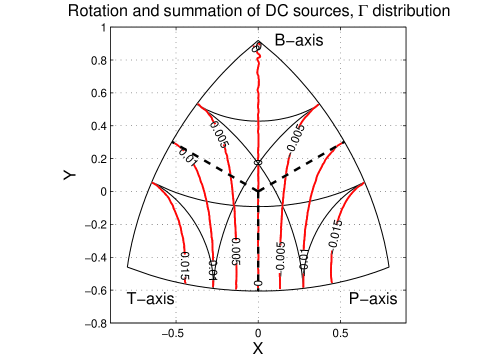
Figure 4: $\Gamma$-index distribution for small rotation angles ($\Phi=10^{\circ}$). See Eq. 46. Two equal DC sources, one rotated compared to another. The axis angles are shown at octant equal-area projection (37); see also (Kagan, 2005). Dashed lines are boundaries between different focal mechanisms. Plunge angles $30^{\circ}$ and $60^{\circ}$ for all mechanisms are shown by thin solid lines.

The first term in the right-hand part of the equation suggests that the invariant reaches maximum in the equatorial plane ($\theta~{}=~{}90^{\circ}$) when the pole coincides with the t- or p-axes ($\phi~{}=~{}0^{\circ}$ or $\phi~{}=~{}90^{\circ}$). Fig. 4 displays the distribution of the $\Gamma$-index for the value of the rotation angle $\Phi=10^{\circ}$ and for equal DC components ($\chi=1.0$).

In calculations we use an approximate formula (46); the exact expression (obtained by mathematica), which is too long to show here, yields almost the same answer. The $\Gamma$-index values in Fig. 4 are very small; thus, a non-zero CLVD component is unlikely to be obtained in the moment solutions for an earthquake consisting of such subevents.

4.2.3 Large rotations

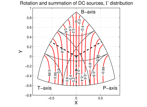
Figure 5: $\Gamma$-index distribution for large rotation angles ($\Phi=90^{\circ}$). Two equal DC sources, one rotated compared to another. Octant projection and auxiliary lines are the same as in Fig. 4.

Formula (46) also suggests that if $\phi=45^{\circ}$, for small values of the rotation angle $\Phi$ and for non-equal DC components the third invariant is proportional to $\sin^{3}(\Phi/2)$, i.e., it is close to zero. In particular, if $\chi=1$, by employing $\phi=45^{\circ}$ in (46), we obtain that $I_{3}\equiv 0$ for arbitrary values of the rotation angle $\Phi$. This means that if the rotation pole is located on a fault- or auxiliary-plane, the sum of two focal mechanisms (original and rotated) has a zero CLVD component, i.e., it is a pure DC source. The effect can be seen in Fig. 5, where the $\Gamma$-index, calculated with the exact formula, is displayed for equal DC components. In this case, if the rotation pole is close to the t- or p-axis, the resulting source is almost pure CLVD.

This property can be demonstrated for a few simple arrangements of sources (see also Frohlich et al., 1989). For example, a sum of two DCs

$${\bf s}\ =\ \left|\begin{array}[]{rrr}1&0&0\\ 0&-1&0\\ 0&0&0\end{array}\right|\ +\ \left|\begin{array}[]{rrr}0&1&0\\ 1&0&0\\ 0&0&0\end{array}\right|\,,$$ (47)

can be rotated into ${\bf s}\,=\,{\rm diag}[\sqrt{2},\,-\sqrt{2},\,0]$ with $I_{3}(s)~{}\equiv~{}0$. This arrangement can be represented as two strike-slip events with a fault-plane rotated by $45^{\circ}$.

Another example is the rotation by $120^{\circ}$ around a pole with coordinates $[1/\sqrt{3},\,1/\sqrt{3},\,1/\sqrt{3}]$, a turn which exchanges the position of coordinate axes.

$${\bf s}\ =\ {\rm diag}[1,\,-1,\,0]\ +\ {\rm diag}[-1,\,0,\,1]\ =\ {\rm diag}[0,\,-1,\,1]\,.$$ (48)

Again $I_{3}(s)\equiv 0$.

For rotation around t-axis, for example,

$${\bf s}\ =\ {\rm diag}[1,\,-1,\,0]\ +\ {\rm diag}[1,\,0,\,-1]\ =\ {\rm diag}[2,\,-1,\,-1]\,.$$ (49)

Such a sum would have $\Gamma=1$, i.e., it is a pure CLVD source (see Fig. 5).

The results above demonstrate that if the rotation pole is located even randomly on nodal-planes, the resulting sum source is a DC. This may be relevant in searching for a non-DC component in seismic moment solutions. Frohlich and Davis (1999) and Kagan (2003) argued that the CLVD component is not presently measured with accuracy sufficient to study its properties.

5 Tensor moment dot product

The tensor dot product has been introduced by Kagan and Knopoff (1985b) as one of the correlation tensor invariants describing a complex earthquake fault pattern. Alberti (2006) used it to characterize the similarity of earthquake focal mechanisms. We compare two methods for characterizing earthquake source complexity: rotation angle $\Phi$ and tensor dot product

$$D\ =\ m_{ij}\,n_{ij};\qquad 2\,\geq\,D\,\geq\,-2\,,$$ (50)

where the second source is rotated with regard to the first by the angle $\Phi$.

The dependence of the product $D$ on 3 parameters of 3-D rotation (26) calculated using mathematica, can be described as

$$D\ = \ 2\,\bigg{\{}\,(\,1-\,{{A}^{2}}\,)^{2}-\,{{A}^{2}}\,{{\cos^{2}(\theta)}}$$ (51)

$$\times\Big{[}\,-6\,+\,6\,{{A}^{2}}\,+\,{{A}^{2}}\,{{\cos^{2}(\theta)}}\Big{]}+\,{{A}^{4}}\,{{\sin^{4}(\theta)}}$$

$$\times\Big{[}{{\cos^{4}(\phi)}}\,-6\,{{\cos^{2}(\phi)}}\,{{\sin^{2}(\phi)}}\,+\,{{\sin^{4}(\phi)}}\,\Big{]}\bigg{\}}\,,$$

where $A$ is given by (44).

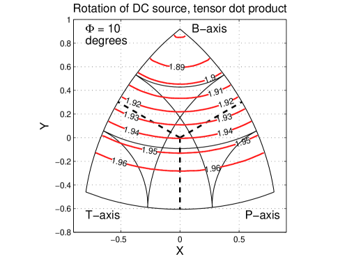
Figure 6: Distribution of the tensor dot product for rotation angle $\Phi=10^{\circ}$. Two equal DC sources, one rotated compared to another. Octant projection and auxiliary lines are the same as in Fig. 4.

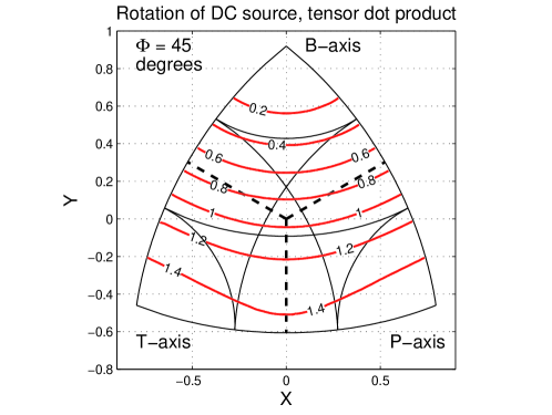
Figure 7: Distribution of the tensor dot product for rotation angle $\Phi=45^{\circ}$. Two equal DC sources, one rotated compared to another. Octant projection and auxiliary lines are the same as in Fig. 4.

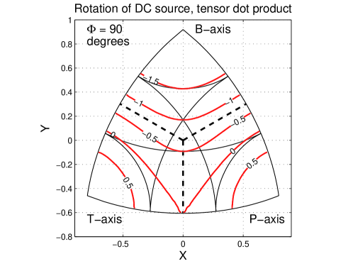
Figure 8: Distribution of the tensor dot product for rotation angle $\Phi=90^{\circ}$. Two equal DC sources, one rotated compared to another. Octant projection and auxiliary lines are the same as in Fig. 4. The $D$-value is $-2$ at the b-axis and $+1$ at the t- and p-axes.

In Figs. 6–8 we display the $D$-value for three choices of the $\Phi$ angle. The maximum change of the $D$-value from $D=2$, corresponding to identical DC sources, occurs when the rotation pole is at the b-axis. For $\Phi=90^{\circ}$ rotation $D=-2$ at the b-axis and $D=1$ for other axes (cf. Eq. 49). Hence, the range of the $D$ change is four times greater for the b-axis rotation than for rotation at other axes. Therefore, from the $D$-value alone we cannot fully infer the complexity and coherence of DC sources. Higher order invariants of the correlation tensor need to be studied to better describe the fault pattern complexity (Kagan, 1992a).

6 Focal mechanisms statistics

The orientation of a DC source can be characterized by the following three quantities: a rotation angle ($\Phi$) of the counterclockwise rotation from the first DC source to the second, and a location of a rotation pole on a reference sphere (26) – colatitude, $\theta$, and longitude, $\phi$ (Kagan 1991, 2003). Thus, to fully study the distribution of earthquake focal mechanisms we need to investigate a six-dimensional manifold (fiber bundle): a product of the 3-D Euclidean space and the 3-D rotational distribution of a DC source. This presents a double difficulty – there is no effective procedure to display and study this pattern and we do not have sufficient data to evaluate the parameters of the six-dimensional distribution.

Therefore, to better analyze the focal mechanism pattern, we should construct only marginal distributions of the full 6-D manifold. The following examples serve to illustrate the theoretical methods described in previous sections.

In Section 6.2 we analyze the distribution of earthquake centroids projected on a focal mechanism reference sphere for each earthquake. Section 6.3 presents the distribution of rotation angles between pairs of DC solutions, and Section 6.4 discusses the statistics of rotation poles.

6.1 Earthquake catalog

We study the earthquake distributions for the global catalog of moment tensor inversions compiled by the CMT group (Ekström et al., 2005, and references therein; see also references and earthquake statistics for 1977-1998 in Dziewonski et al., 1999). The catalog contains 26,865 solutions over a period from 1977/1/1 to 2007/3/31. Only shallow earthquakes (depth 0-70 km) are studied here.

The CMT catalog includes seismic moment centroid times and locations as well as estimates of seismic moment tensor components (Dziewonski et al., 1981; Dziewonski and Woodhouse, 1983). Each tensor is constrained to have zero trace (first invariant), i.e., no isotropic component. Double-couple (DC) solutions, i.e., with tensor determinant equal to zero, are supplied as well. Almost all earthquake parameters are accompanied by internal estimates of error.

From the original CMT catalog we created subcatalogs of well-constrained solutions. These datasets are obtained by removing from the catalog (a) the earthquakes lacking all 6 independent components of the moment tensor, (b) solutions with a large relative error, and (c) the solutions with large CLVD component (Frohlich and Davis, 1999; Kagan, 2000). Since the larger earthquakes usually have smaller errors (Kagan, 2003), fewer of these events are removed. About 85% of $m\geq 6.0$ earthquakes are well-constrained, whereas for smaller earthquakes ($m\geq 5.0$) more than 2/3 have been deleted.

6.2 Centroid distribution on a focal sphere

Similarly to Table 1 in Kagan (1992b) in Table 1 here we show the distribution of numbers of centroids in a coordinate system formed by the t-, p-, and b-axes of earthquake focal mechanisms. Each quadrant of the focal sphere is subdivided into 110 spherical triangles and quadrilaterals with equal area (consequently covering equal solid angles), and we calculate the number of times a centroid in projected into these cells. We normalize the numbers, so that the total number of the entries of Table 1 equals 11,000. Therefore, if the distribution of centroids in the tpb-system were completely random, all the numbers in the table would be equal to 100. The entries ‘Col. Angle’ give the colatitude angle corresponding to the lower edge of a segment consisting of one or several cells. The number of pairs for each segment is shown in ‘Pair number’ column.

Table 1 shows a strong concentration of centroids near the plane going through the t–p and the b-vectors. Therefore this plane should correspond to the fault-plane and that going through the t+p and b-vectors should usually correspond to the auxiliary plane. Most of the strong earthquakes are concentrated in subduction zones. Fig. 3 in Kagan and Jackson (1994) illustrates that the fault-plane should include both the t–p and the b-vectors.

Huc and Main (2003) suggest that the vertical errors in centroid determination would strongly influence the direction statistics between the pairs of events. Even for $M6$ earthquakes, about 1/3 of shallow centroids are assigned the depth of 15 km. This means that the depth could not be accurately evaluated.

These results and those shown in Table 1 by Kagan (1992b) support the conventional model of an earthquake fault: a rupture propagating with slight deviations along a fault-plane. Figs. 3 and 4 suggest that an earthquake occurring on such a fault system should have the CLVD component close to zero even if subevent focal mechanisms are significantly disoriented by rotation around the axis normal to the fault-plane (n-axis).

6.3 Rotation angle statistics

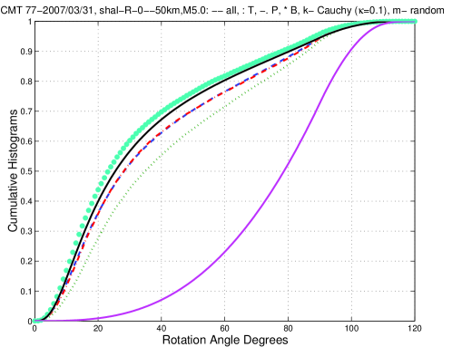
Figure 9: Distributions of rotation angles for pairs of focal mechanisms of shallow earthquakes (depth 0-70 km) in the CMT catalog 1977/01/01–2007/03/31; centroids are separated by distances between 0-50 km, magnitude threshold $m_{w}=5.0$. Circles – all centroids ; crosses – centroids in 30^∘ cones around the t-axis; plusses – centroids in 30^∘ cones around the p-axis; stars – centroids in 30^∘ cones around the b-axis. Left solid line is for the Cauchy rotation with $\kappa=0.1$; right solid line is for the random rotation.

Fig. 9 displays cumulative distributions of the rotation angle $\Phi$ for shallow earthquake pairs separated by a distance of less than 50 km. We study whether the rotation of focal mechanisms depends on where the second earthquake of a pair is situated with regard to the first event. Thus we measure the rotation angle for centroids located in 30^∘ cones around each principal axis (see curves, marked the t-, p-, and b-axes) of the first event.

The curves in Fig. 9 are narrowly clustered, and are obviously well approximated by the DC rotational Cauchy distribution (Kagan, 1990, 1992b). This distribution is characterized by a parameter $\kappa$; a smaller $\kappa$-value corresponds to the rotation angle $\Phi$ concentrated closer to zero. Thus, all earthquakes, regardless of their spatial orientation, have focal mechanisms similar to a close event. Earthquakes in the cone around the b-axis correspond to a smaller $\kappa$-value than the events near the other axes. These results are similar to the results shown in Fig. 6 by Kagan (1992b).

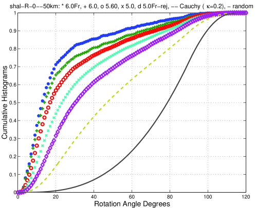
Figure 10: Distributions of rotation angles for pairs of focal mechanisms of shallow earthquakes in the CMT catalog; centroids are separated by distances between 0-50 km; centroids in 30^∘ cones around the b-axis. Stars – CMT well-constrained earthquakes, magnitude threshold $m_{t}=6.0$, 1977/01/01–2005/01/01; plusses – CMT catalog, magnitude threshold $m_{t}=6.0$, 1977/01/01–2007/03/31; circles – CMT catalog, magnitude threshold $m_{t}=5.6$, 1977/01/01–2007/03/31; crosses – CMT catalog, magnitude threshold $m_{t}=5.0$, 1977/01/01–2007/03/31; diamonds – CMT not well-constrained earthquakes, magnitude threshold $m_{t}=5.0$, 1977/01/01–2005/01/01. Left dashed line is for the Cauchy rotation with $\kappa=0.2$; right solid line is for the random rotation.

In Fig. 10 we show how the distribution of the rotation angle $\Phi$ depends on the magnitude threshold and the selection of the well-constrained earthquakes in the catalog (Section 6.1). It is clear from the diagram that 1) for larger earthquakes the angle distribution is generally more concentrated near zero, and 2) the well-constrained earthquakes also have a smaller angle between pairs. These conclusions are easily explained by the higher accuracy of strong event solutions (Kagan, 2003): the disorientation of the DC solutions is caused mostly by solution errors. Kagan (2000) indicates that the rotation angle error is on the order $10^{\circ}$ for the best solutions. Fig. 4 suggests that if subevent constituents of an earthquake have small rotation ($\Phi\leq 10^{\circ}$), the CLVD component would be close to zero.

Below we show the pattern analysis for the most accurate solutions: the well-constrained earthquakes $m\geq 6.0$. The disadvantage here is their small number.

6.4 Rotation pole statistics

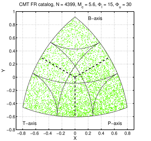
Figure 11: Distributions of rotation poles for pairs of focal mechanisms of shallow well-constrained earthquakes in the CMT 1977/01/01–2005/01/01 catalog. Centroids are separated by distances between 0-50 km; magnitude threshold $m_{t}=5.6$; the rotation angle $15^{\circ}\leq\Phi\leq 30^{\circ}$.

From Figs. 4–5 one can infer that the rotation pole position strongly influences the CLVD component of a complex source. In Fig. 11 we show the distribution of the rotation poles for the second earthquake focal mechanism on a reference sphere of the first event. Because of the symmetry of the DC source, we reflect the point pattern at our reference sphere at the planes perpendicular to all axes. Thus, the distribution can be shown on an octant of a sphere. We use the Lambert azimuthal equal-area projection (37).

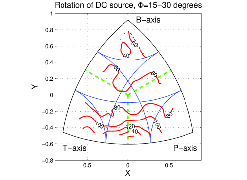
Figure 12: Map of rotation poles for pairs of focal mechanisms of shallow well-constrained earthquakes in the CMT catalog, see Fig. 11.

For example, if in Fig. 11, a pole is shown near the b-axis, this would mean that in both mechanisms the axis has almost the same orientation: the second mechanism is rotated by an angle $\Phi$ around an axis intersecting the sphere at the pole. The same pattern occurs for the poles that are close to other axes. In the diagram, the angle is $15^{\circ}\leq\Phi\leq 30^{\circ}$. The points seem to concentrate between t- and p-axes. Fig. 12 shows the point density distribution, again confirming that the greatest pole concentration is located near a nodal-plane.

In Table 2 we display the distributions of the rotation poles on a reference sphere of the first event. In this Table, as in Table 1, we subdivide the positive octant of the sphere into 55 spherical triangles and quadrilaterals with equal area and then calculate the number of times the rotation axis intersects each of these cells.

The upper chart in Table 2 shows the distribution of axes for the rotation angles of less than 15^∘. The distribution is randomly uniform as can be expected, because these rotations are caused, most probably, by random errors. For larger angles (the second chart, $15^{\circ}\leq\Phi\leq 30^{\circ}$) the distribution shows that the stresses of the first earthquake influence the focal mechanism of the second earthquake in a pair.

To illustrate the data and our technique in Table 3, we show the calculations for 18 pairs of earthquakes in the lower-left corner cell of the second chart in Table 2. Earthquakes are distributed more or less uniformly at subduction zones. We can see again that many of them have been assigned the standard depth of 15 km. As explained above in this Subsection, the t-axes of both solutions are almost identical. Therefore, the rotation poles are concentrated near the axis projection, both in Table 2 and in Fig. 11. Because the rotation angle is relatively small ($15^{\circ}\leq\Phi\leq 30^{\circ}$) the p-axes also have close orientation.

However, the third and fourth charts of the Table calculated for the large angles of rotation display a different behaviour. The rotation poles are concentrated near the b- and p-axes. Inspection of these earthquake pairs indicates that 20 of 41 duos are concentrated in an area 200 by 200 km near the New Hebrides Islands – a region of complex subduction tectonics. These earthquakes likely result from the complicated slab geometry.

We note that in Table 7 in Kagan (1992b) which is similar to Table 2, the plane orthogonal to the b-axis was incorrectly rotated by 90^∘ and the results collapsed on an octant. Therefore, the number pattern at the former Table rows at p- and t-axis is a mixture of both distributions.

7 Discussion

We studied the distribution of the non-DC (CLVD) component for a composite earthquake source or a fault system. A source is considered complex if it consists of two or more events with a DC focal mechanism differently oriented. The theoretical computations detail conditions under which such a source would produce a non-zero CLVD component. For most of the geometric barriers proposed as common features in an earthquake fault system (King, 1983, 1986), the CLVD component should be zero. Frohlich et al. (1989) and Frohlich (1990) came to similar conclusions.

We tried to statistically estimate whether the geometrical pattern leading to a zero CLVD could be confirmed by analyzing an earthquake catalog of focal mechanism solutions. However, the results shown in the previous Section are not fully convincing. They do, however, suggest limited support for this conjecture.

Why can’t analysis of earthquake focal mechanisms in available catalogs definitively explain the CLVD component presence? To understand shear rupture properties, we need to investigate the behavior of the seismic moment tensor sums for distances between events close to zero. At such distances, the intrinsic geometrical conditions of the rupture would play a major role. At larger distances the slab geometry and its interaction with the upper mantle would significantly influence the focal mechanisms and pattern of earthquake hypocenters/centroids. Moreover, because of the low frequency waves used in the seismic moment inversion, centroids in the CMT catalog have low accuracy both in the horizontal plane and at depth. From Smith and Ekström’s (1997) and Kagan’s (2003) results, horizontal accuracy in a centroid location can be estimated on the order of 15-20 km. Centroid depth uncertainty should be the same or higher. In our computations we use distances between the events, which should increase the random error but decrease systematic uncertainties. The accuracy values quoted above are comparable with the slab thickness. This means that our distributions are influenced strongly by slab geometry.

Brudzinski et al. (2007) studied slab geometry for the subduction zones using higher accuracy (less than 10 km, see above) hypocentral global earthquake catalogs. They found that earthquakes concentrate at two layers: double Benioff zones or the upper and lower boundaries of a subducting slab. This means that large earthquakes which are listed in the CMT catalog are mostly connected with the subducting plate geometry, not with any local geometry of the rupture zone. The geometry of deforming thin elastic sheets of material is a complex problem even if the sheet is deforming in free space (Marder et al., 2007).

For earthquakes occurring at the double Benioff zones, the treatment of focal mechanisms should be modified because their symmetry properties differ from those of earthquakes in the middle of a slab. For DC sources of earthquakes at the slab boundary, we should be able, in principle, to identify not only which of the focal planes is a fault-plane, but also to resolve the “up and down” of the fault-plane (Kagan, 1990, p. 576). Hence, the only symmetry operation for such a focal mechanism is the identity (23). In such a case, the quaternion visualization techniques described by Hanson (2005, Ch. 21-23) can be implemented to picture both a slab surface geometry and the frames of earthquake rupture associated with the surface. However, the techniques proposed above are developed for smooth rotations. As we indicated earlier (Section 1.2) earthquakes occur on fractal sets and the orientation of their focal mechanisms is also controlled by a non-smooth fractal distribution. Therefore, new methods need to be created for displaying earthquake focal mechanisms and their spatial pattern.

While investigating earthquake spatial distribution (Kagan, 2007a), we were able in some degree to make a smooth transition from a 3-D distribution of hypocenters for small distances to a 2-D epicenter distribution for distances comparable or larger than the thickness of seismogenic crust. After appropriate adjustments, the obtained values of fractal dimension are comparable for both cases. It seems, however, that the methods employed for simple point distributions in 2-D and 3-D are much more difficult to implement for tensor quantities. The challenges are two-fold: theoretical problems of displaying and interpreting the 6-D distributions and the more practical problem of no high quality, massive datasets of focal mechanism solutions.

Several extensive local catalogs of focal mechanism solutions have been compiled (Pasyanos et al., 1996; Kubo et al., 2002; Hardebeck, 2006; Clinton et al., 2006; Matsumoto et al., 2006). They contain thousands of events. Many of these occur near local seismographic stations and, therefore, their solutions have good depth control. However, the largest catalogs are based on first-motion analysis and their solutions have a significantly lower accuracy than do catalogs of the moment-tensor inversions (Kagan, 2002, 2003). The latter catalogs are not yet sufficiently extensive, well-documented, or tested to be used for rigorous statistical studies. However, it is possible that in a few years these catalogs will be improved.

Figure 1: Schematic diagrams of earthquake focal mechanism. Equal-area projection (Aki and Richards, 2002, p. 110) of quadrupole radiation patterns. The null (b) axis is orthogonal to the t- and p-axes, or it is located on the intersection of fault and auxiliary planes, i.e., perpendicular to the paper sheet in this display.

Figure 2: Schematic diagrams of earthquake focal zone. Lines show a complex fault plane; focal mechanisms of earthquake(s) are displayed for each fault segments. (a) Rotation around b-axis, non-conservative geometric barriers. (b) Rotation around u-axis (slip vector), conservative geometric barriers.

Figure 3: Schematic diagrams of earthquake focal zone. Rotation around n-axis (fault-plane normal vector), conservative geometric barrier. (c) View from side. (d) View from above.

References

- [1] Abramowitz, M. and I. A. Stegun (1972), Handbook of Mathematical Functions, Dover, NY, pp. 1046.
- [2] Aki, K. and Richards, P., 2002. Quantitative Seismology, 2nd ed., Sausalito, Calif., University Science Books, 700 pp.
- [3] Alberti, M., 2006. Spatial structures in earthquakes and faults: quantifying similarity in simulated stress fields and natural data sets, J. Structural Geol., 28(6), 998-1018.
- [4] Altmann, S. L., 1986. Rotations, Quaternions and Double Groups, Clarendon Press, Oxford, pp. 317.
- [5] Amelung, F., and G. King, 1997. Large-scale tectonic deformation inferred from small earthquakes, Nature, 386, 702-705.
- [6] Anderson, T. L., 2005. Fracture Mechanics: Fundamentals and Applications, 3rd ed., Boca Raton, Taylor and Francis.
- [7] Backus, G. E., 1977a. Interpreting the seismic glut moments of total degree two or less, Geophys. J. R. astr. Soc., 51, 1-25.
- [8] Backus, G. E., 1977b. Seismic sources with observable glut moments of spatial degree two, Geophys. J. R. astr. Soc., 51, 27-45.
- [9] Backus, G. and Mulcahy, M., 1976a. Moment tensor and other phenomenological descriptions of seismic sources – I. Continuous displacements. Geophys. J. R. astr. Soc., 46, 341-361.
- [10] Backus, G. and Mulcahy, M., 1976b. Moment tensor and other phenomenological descriptions of seismic sources – II. Discontinuous displacements. Geophys. J. R. astr. Soc., 47, 301-329.
- [11] Bressan, G., Bragato, P.L., and Venturini, C., 2003. Stress and strain tensors based on focal mechanisms in the seismotectonic framework of the Friuli-Venezia Giulia region (Northeastern Italy), Bull. Seismol. Soc. Amer., 93(3), 1280-1297.
- [12] Brudzinski, M. R., C. H. Thurber, B. R. Hacker, and E. R. Engdahl, 2007. Global Prevalence of Double Benioff Zones, Science, 316(5830), 1472 - 1474, [DOI: 10.1126/science.1139204]
- [13] Burridge, R. and Knopoff, L., 1964. Body force equivalents for seismic dislocations, Bull. Seismol. Soc. Amer., 54, 1875-1888.
- [14] Chen, P., T.H. Jordan, L. Zhao, 2005. Finite-moment tensor of the 3 September 2002 Yorba Linda earthquake, Bull. Seismol. Soc. Amer., 95(3), 1170-1180.
- [15] Clinton, J. F., E. Hauksson, and K. Solanki, 2006. An Evaluation of the SCSN Moment Tensor Solutions: Robustness of the Magnitude Scale, Style of Faulting, and Automation of the Method, Bull. Seismol. Soc. Amer., 96(5), 1689-1705.
- [16] Dreger, D. S., 2003. TDMT_INV: Time Domain Seismic Moment Tensor INVersion, International Handbook of Earthquake and Engineering Seismology, (W. H. K. Lee, H. Kanamori, P. C. Jennings, and C. Kisslinger, Editors), Volume B, Chapter 81, p. 1627.
- [17] Dziewonski, A. M., G. Ekström, and N. N. Maternovskaya, 1999. Centroid-moment tensor solutions for October-December, 1998. Phys. Earth Planet. Inter., 115, 1-16.
- [18] Dziewonski, A. M., and Woodhouse, J. H., 1983. An experiment in systematic study of global seismicity: centroid-moment tensor solutions for 201 moderate and large earthquakes of 1981, J. Geophys. Res., 88, 3247-3271.
- [19] Dziewonski, A. M., Chou, T.-A., and Woodhouse, J. H., 1981. Determination of earthquake source parameters from waveform data for studies of global and regional seismicity, J. Geophys. Res., 86, 2825-2852.
- [20] Ekström, G., A. M. Dziewonski, N. N. Maternovskaya and M. Nettles, 2005. Global seismicity of 2003: Centroid-moment-tensor solutions for 1087 earthquakes, Phys. Earth Planet. Inter., 148(2-4), 327-351.
- [21] Fineberg, J., E. Sharon, and G. Cohen, 2003. Crack front waves in dynamic fracture, International Journal of Fracture, 119(3), 247-261.
- [22] Frohlich, C., 1990. Note concerning non-double-couple source components from slip along surfaces of revolution, J. Geophys. Res., 95(B5), 6861-6866.
- [23] Frohlich, C., 2006. Deep Earthquakes, New York, Cambridge University Press, 573 pp.
- [24] Frohlich, C., and S. D. Davis, 1999. How well constrained are well-constrained T, B, and P axes in moment tensor catalogs?, J. Geophys. Res., 104, 4901-4910.
- [25] Frohlich, C., M. A. Riedesel, and K. D. Apperson, 1989. Note concerning possible mechanisms for non-double-couple earthquake sources, Geophys. Res. Lett., 16(6), 523-526.
- [26] Gabrielov, A., Keilis-Borok, V., and Jackson, D. D., 1996. Geometric incompatibility in a fault system, P. Natl. Acad. Sci. USA, 93, 3838-3842.
- [27] Hanson, A. J., 2005. Visualizing Quaternions, San Francisco, Calif., Elsevier, pp. 498.
- [28] Hardebeck, J. L., 2006. Homogeneity of Small-Scale Earthquake Faulting, Stress, and Fault Strength, Bull. Seismol. Soc. Amer., 96(5), 1675-1688.
- [29] Huc, M., and I. G. Main, 2003. Anomalous stress diffusion in earthquake triggering: Correlation length, time dependence, and directionality, J. Geophys. Res., 108(B7), ESE-1, pp. 1-12, art. no. 2324.
- [30] Jaeger, J. C., and N. G. W. Cook, 1979. Fundamentals of Rock Mechanics, 3-rd ed., Chapman and Hall, London, 593 pp.
- [31] Julian, B. R., A. D. Miller, G. R. Foulger, 1998. Non-double-couple earthquakes, 1. Theory, Rev. Geophys., 36(4), 525-549.
- [32] Kagan, Y. Y., 1982. Stochastic model of earthquake fault geometry, Geophys. J. Roy. astr. Soc., 71, 659-691.
- [33] Kagan, Y. Y., 1987. Point sources of elastic deformation: Elementary sources, static displacements, Geophys. J. Roy. astr. Soc., 90, 1-34. (Errata, Geophys. J. R. Astron. Soc., 93, 591, 1988.)
- [34] Kagan, Y. Y., 1988. Static sources of elastic deformation in homogeneous half-space, J. Geophys. Res., 93, 10,560-10,574.
- [35] Kagan, Y. Y., 1990. Random stress and earthquake statistics: Spatial dependence, Geophys. J. Int., 102, 573-583.
- [36] Kagan, Y. Y., 1991. 3-D rotation of double-couple earthquake sources, Geophys. J. Int., 106, 709-716.
- [37] Kagan, Y. Y., 1992a. On the geometry of an earthquake fault system, Phys. Earth Planet. Inter., 71(1-2), 15-35.
- [38] Kagan, Y. Y., 1992b. Correlations of earthquake focal mechanisms, Geophys. J. Int., 110, 305-320.
- [39] Kagan, Y. Y., 2000. Temporal correlations of earthquake focal mechanisms, Geophys. J. Int., 143, 881-897.
- [40] Kagan, Y. Y., 2002. Modern California earthquake catalogs and their comparison, Seism. Res. Lett., 73(6), 921-929.
- [41] Kagan, Y. Y., 2003. Accuracy of modern global earthquake catalogs, Phys. Earth Planet. Inter., 135(2-3), 173-209.
- [42] Kagan, Y. Y., 2005. Double-couple earthquake focal mechanism: Random rotation and display, Geophys. J. Int., 163(3), 1065-1072.
- [43] Kagan, Y. Y., 2006. Why does theoretical physics fail to explain and predict earthquake occurrence?, Lecture Notes in Physics, 705, pp. 303-359, P. Bhattacharyya and B. K. Chakrabarti (Eds.), Springer Verlag, Berlin–Heidelberg. http://scec.ess.ucla.edu/ykagan/india_index.html
- [44] Kagan, Y. Y., 2007a. Earthquake spatial distribution: the correlation dimension, Geophys. J. Int., 168(3), 1175-1194.
- [45] Kagan, Y. Y., 2007b. Simplified algorithms for calculating double-couple rotation, Geophys. J. Int., 171(1), 411-418.
- [46] Kagan, Y. Y., and D. D. Jackson, 1994. Long-term probabilistic forecasting of earthquakes, J. Geophys. Res., 99, 13,685-13,700.
- [47] Kagan, Y. Y., and L. Knopoff, 1985a. The first-order statistical moment of the seismic moment tensor, Geophys. J. Roy. astr. Soc., 81, 429-444.
- [48] Kagan, Y. Y., and L. Knopoff, 1985b. The two-point correlation function of the seismic moment tensor, Geophys. J. Roy. astr. Soc., 83, 637-656.
- [49] King, G., 1983. The accommodation of large strains in the upper lithosphere of the Earth and other solids by self-similar fault systems: the geometrical origin of -value, Pure Appl. Geophys., 121, 761-815.
- [50] King, G.C.P., 1986. Speculations on the geometry of the initiation and termination processes of earthquake rupture and its relation to morphology and geological structure, Pure Appl. Geophys., 124(3), 567-585.
- [51] Klein, F., 1932. Elementary Mathematics from an Advanced Standpoint. Vol. I. Arithmetic, Algebra, Analysis, transl. by E. R. Hedrick and C. A. Noble, Macmillan, London, pp. 274.
- [52] Knopoff, L. and Randall, M. J., 1970. The compensated linear vector dipole: A possible mechanism for deep earthquakes, J. Geophys. Res., 75, 4957-4963.
- [53] Kubo, A., E. Fukuyama, H. Kawai, and K. Nonomura, 2002. NIED seismic moment tensor catalogue for regional earthquakes around Japan: quality test and application, Tectonophysics, 356, 23-48.
- [54] Kuffner, J., 2004. Effective Sampling and Distance Metrics for 3D Rigid Body Path Planning, Proceedings 2004 IEEE Internat. Conference on Robotics and Automation, 4, 3993-3998, New Orleans, LA.
- [55] Kuipers, J. B., 2002. Quaternions and Rotation Sequences: A Primer with Applications to Orbits, Aerospace and Virtual Reality, Princeton, Princeton Univ. Press., 400 pp.
- [56] Marder, M., Deegan, R. D., and Sharon, E., 2007. Crumpling, buckling, and cracking: Elasticity of thin sheets, Physics Today, 60(2), 33-38.
- [57] Marsaglia, G., 1972. Choosing a point from the surface of a sphere, Ann. Math. Stat., 43, 645-646.
- [58] MathWorks, 2006. Aerospace Toolbox – Quaternion Math, http://www.mathworks.com/access/helpdesk/help/toolbox/aerotbx/ (see Functions – By Category, then Quaternion Math)
- [59] MathWorld, 2004. http://mathworld.wolfram.com/Quaternion.html
- [60] Matsumoto T, Ito Y, Matsubayashi H, Sekiguchi S., 2006. Spatial distribution of F-net moment tensors for the 2005 West Off Fukuoka Prefecture Earthquake determined by the extended method of the NIED F-net routine, Earth Planet. Space, 58(1), 63-67.
- [61] McGuire, J. J., Li Zhao, and Jordan, T. H., 2001. Teleseismic inversion for the second-degree moments of earthquake space-time distributions, Geophys. J. Int., 145, 661-678.
- [62] Miller, A. D., G. R. Foulger, B. R. Julian, 1998. Non-double-couple earthquakes 2. Observations, Rev. Geophys., 36(4), 551-568.
- [63] Moran, P. A. P., 1975. Quaternions, Haar measure and estimation of paleomagnetic rotation, in: Perspectives in Probability and Statistics, (ed. J. Gani), Acad. Press, 295-301.
- [64] Pasyanos, M. E., D. S. Dreger, and B. Romanowicz, 1996. Toward real-time estimation of regional moment tensors, Bull. Seismol. Soc. Amer., 86, 1255-1269.
- [65] Pondrelli, S., S. Salimbeni, G. Ekström, A. Morelli, P. Gasperini and G. Vannucci, 2006. The Italian CMT dataset from 1977 to the present, Phys. Earth Planet. Inter., 159, 286-303.
- [66] Ponson, L., D. Bonamy, H. Auradou, G. Mourot, S. Morel, E. Bouchaud, C. Guillot, and J.P. Hulin, (2006). Anisotropic self-affine properties of experimental fracture surfaces, International Journal of Fracture, 140(1-4), 27-37.
- [67] Richardson, E., and T. H. Jordan, 2002. Low-frequency properties of intermediate-focus earthquakes, Bull. Seismol. Soc. Amer., 92(6), 2434-2448.
- [68] Roessler, D., Krueger, F., and Ruempker, G., 2007. Retrieval of moment tensors due to dislocation point sources in anisotropic media using standard techniques, Geophys. J. Int., 169(1), 136-148.
- [69] Shen, Y.-Z., Y. Chen, D.-H. Zheng, 2006. A quaternion-based geodetic datum transformation algorithm, J. Geod., 80, 233-239, DOI 10.1007/s00190-006-0054-8.
- [70] Silver, P. G., and Jordan, T. H., 1983. Total-moment spectra of fourteen large earthquakes, J. Geophys. Res., 88, 3273-3293.
- [71] Silver, P. and Masuda, T., 1985. Source extent analysis of the Imperial Valley earthquake of October 15, 1979, and the Victoria earthquake of June 9, 1980, J. Geophys. Res., 90, 7639-7651.
- [72] Smith, G. P., and G. Ekström, 1997. Interpretation of earthquake epicenter and CMT centroid locations, in terms of rupture length and direction, Phys. Earth Planet. Inter., 102, 123-132.
- [73] Snoke, J. A., 2003. FOCMEC: FOcal MEChanism determinations, International Handbook of Earthquake and Engineering Seismology (W. H. K. Lee, H. Kanamori, P. C. Jennings, and C. Kisslinger, Eds.), Academic Press, San Diego, Chapter 85.12. http://www.geol.vt.edu/outreach/vtso/focmec/
- [74] Snyder, J. P., 1987. Map Projections – A Working Manual, U.S. Geological Survey professional paper, 1395; Washington, 383 pp.
- [75] Stein, S., and E. Klosko, 2003. Earthquake mechanism and plate tectonics, in IASPEI Handbook of Earthquake and Engineering Seismology (W. H. K. Lee, H. Kanamori, P. C. Jennings, and C. Kisslinger, Editors), pp. 69-78, Boston, Academic Press.
- [76] Ward, J. P., 1997. Quaternions and Cayley Numbers: Algebra and Applications, Kluwer Acad. Pub., London, pp. 237.
- [77] Wolfram, S., 1999. The Mathematica Book, 4th ed., Champaign, IL, Wolfram Media, Cambridge, New York, Cambridge University Press, pp. 1470.
- [78] Yershova, A., and S. M. LaValle, 2004. Deterministic Sampling Methods for Spheres and SO(3), Proceedings 2004 IEEE Internat. Conference on Robotics and Automation, 4, 3974-3980, New Orleans, LA.