Universality in movie rating distributions

Abstract

In this paper histograms of user ratings for movies ($1\bigstar,\dots,10\bigstar$) are analysed. The evolving stabilised shapes of histograms follow the rule that all are either double- or triple-peaked. Moreover, at most one peak can be on the central bins $2\bigstar,\dots,9\bigstar$ and the distribution in these bins looks smooth ‘Gaussian-like’ while changes at the extremes ($1\bigstar$ and $10\bigstar$) often look abrupt. It is shown that this is well approximated under the assumption that histograms are confined and discretised probability density functions of Lévy skew $\alpha$-stable distributions. These distributions are the only stable distributions which could emerge due to a generalized central limit theorem from averaging of various independent random variables as which one can see the initial opinions of users. Averaging is also an appropriate assumption about the social process which underlies the process of continuous opinion formation. Surprisingly, not the normal distribution achieves the best fit over histograms obseved on the web, but distributions with fat tails which decay as power-laws with exponent $-(1+\alpha)$ ($\alpha=\frac{4}{3}$). The scale and skewness parameters of the Lévy skew $\alpha$-stable distributions seem to depend on the deviation from an average movie (with mean about $7.6\bigstar$). The histogram of such an average movie has no skewness and is the most narrow one. If a movie deviates from average the distribution gets broader and skew. The skewness pronounces the deviation. This is used to construct a one parameter fit which gives some evidence of universality in processes of continuous opinion dynamics about taste.

1 Introduction

Are there universal laws underlying the dynamics of opinion formation?

Understanding opinion formation is tackled classically by social psychologists and sociologists with experiments (see e.g. Asch1955Opinionsandsocial ; Lorge.Fox.ea1958surveyofstudies ; Sherif.Hovland1961SocialJudgmentAssimilation ; Forgas1977Polarisationandmoderation ; Friedkin1999ChoiceShiftand ; Salganik.Dodds.ea2006ExperimentalStudyof ; Mason.Conrey.ea2007SituatingSocialInfluence ), but also by the social simulation (see e.g. Deffuant.Neau.ea2000MixingBeliefsamong ; Hegselmann.Krause2002OpinionDynamicsand ; Urbig2003AttitudeDynamicswith ; Deffuant.Neau.ea2002HowCanExtremism ; Jager.Amblard2004UniformityBipolarizationand ; Salzarulo2006ContinuousOpinionDynamics ; Baldassarri.Bearman2007DynamicsofPolitical ) and sociophysics (see surveys Stauffer2005SociophysicssimulationsII ; Lorenz2007ContinuousOpinionDynamics ; Castellano.Fortunato.ea2007Statisticalphysicsof ) communities. Often studies are either empirical but on small experimental samples or contrary they analyse models analytically or by simulation but without empirical validation. Both restricts the possibility to draw conclusions on universality in real world opinion formation. This is to a large extent due to the difficulties in getting large scale data on human opinions. But this situation changes rapidly nowadays thanks to the world wide web. The existence of rating modules is almost ubiquitous. (In the meantime the ubiquity of ratings has raised the question how to standardise rating modules Turnbull2007Ratingvoting .)

This paper is an attempt to exploit rating data to extract universal properties in opinion formation processes. Specifically, the focus here is on opinions about the quality of movies, as expressed by users on movie rating sites. Ratings stand as a proxy for any opinion related to taste which is one-dimensional and of a continuous nature (‘continuous’ means expressible as a real number and also gradually adjustable (at least to some extent)). Apparently, possible user ratings are discrete ($1\bigstar$(awful), $\dots$, $10\bigstar$(excellent)), but the continuous nature (in the sense of ordered numbers) is also obvious.

Thus, this paper is not about discrete opinion dynamics without a continuous nature (like e.g. with respect to decision: ‘yes’ or ‘no’) as often studied in physics because of the analogy to spin systems. This paper is also not on multidimensional many-faceted opinions (as e.g. Lorenz2008ManagingComplexityInsights ; Baldassarri.Bearman2007DynamicsofPolitical ) but on issues which are broken down to one variable: the quality of a movie. It is also important to distinguish the type of opinion. Movie ratings are about taste. There is no true value as for example in issues of fact-finding about an unknown quantity. Further on, there is no real physical constraint for opinions. It is always possible to like a movie more than someone else. This is for example not the case in opinions about budgeting in the political realm, where opinions have to be within certain bounds. Finally, taste differs from issues about negotiations where there is a clear incentive of agreeing on a common value (as e.g. for prices in trade, or forming a politcal party in political issues). In issues of taste there is nevertheless a weaker force to adjust towards the opinions of peers, e.g. for normative reasons (‘I’d like to like what my peers like.’). But there might also be a force to adjust away from the opinions of others to pronounce individuality.

User ratings on the world wide web have already been subject of research. Dellarocas Dellarocas2003DigitizationofWord sketches their role for digitising Word-of-Mouth (with the main focus on reputation mechanisms). Ratings play a key role in some recommendation algorithms, see Goldberg et al Goldberg.Roeder.ea2001EigentasteConstantTime , Cheung et al Cheung.Kwok.ea2003Miningcustomerproduct , and Umayarov et al Umyarov.Tuzhilin2007Leveragingaggregateratings which work by comparing the rating profiles of different users. They also play a role in a recent method of pricing an option on movie revenues, see Chance et al Chance.Hillebrand.ea2008PricingOptionRevenue . Salganik et al Salganik.Dodds.ea2006ExperimentalStudyof study the emerging popularity of songs measured by downloads under the impact of the visibility of the number of downloads. They used ratings to check if liking corresponds to downloads, which is the case. But which movie gets popular is to some extend arbitrary.

Jiang and Chen Jiang.Chen2007EconomicAnalysisof argue economically that the implementation of online rating systems can enhance consumer surplus, vendor profitability and social welfare. But they also argue, that this could work better in a monopolistic market than a duopolistic market.

Cosley et al Cosley.Lam.ea2003Isseeingbelieving checked how users re-rate movies especially if they are confronted with a prediction of the quality (like the mean of other ratings). They found a tendency to adjust towards the presented prediction. They also show that users rate quite consistently when they re-rate on other scales (like $5\bigstar$ compared to $10\bigstar$).

Li and Hitt Li.Hitt2004SelfSelectionand analysed the time evolution of the user reviews arriving. (A review is a text but it is accompanied by a rating is assigned by the writer.) They present an economic model where the utility of a product for a user is determined by individual search attributes which are known before purchase and individual quality which can only be checked after purchase. Both attributes are heterogeneous across the population and purchasing decisions are made with respect to expected quality. Expectations can be influenced by user reviews. Positive reviews of early adopters produce high average ratings and thus too high expected quality. This triggers purchases of other consumers which then get disappointed and write bad reviews. If individual search attributes towards a product are positively correlated with individual quality then this may imply a declining trend of reviews. This is called positive self selection bias. Negative correlations imply negative self selection bias and thus an increasing trend of reviews. These trends are confirmed empirically by book review data on amazon.com with the majority of products (70%) showing positive self selection.

The phenomenon of declining average votes has been explained in a different way in Wu.Huberman2008PublicDiscoursein . They argue from the point of view of the writer in front of a computer. Writing a review is costly (in terms of time) and writers want to impact the average vote. While the average vote over all books is more positive one can only make a difference with a negative review, so writers with a positive attitude hesitate to write a review. (If there are already a lot, so why write another?) They also emphasize that internet reviews do not show a group polarization effect which is known to appear in small groups discussing in the same physical roomFriedkin1999ChoiceShiftand .

There are few studies on characterising the empirical distributions of ratings. In Dellarocas.Narayan2006StatisticalMeasureof histograms of user-ratings (on $5\bigstar$-scale in movies.yahoo.com) are characterised as U-shaped, while professional critics have a single-peaked usage of the votes (peak is at 4). Other studies concentrate either on user profile comparison or only on the average vote and how it could impact further votes and sales. In models idiosyncratic opinions are very often thought to be normal distributed Borghesi.Bouchaud2007Ofsongsand ; Gu.Lin2006DynamicsOFOnline ; Umyarov.Tuzhilin2007Leveragingaggregateratings . In the model of Li.Hitt2004SelfSelectionand the beta distribution is used which lives on a bounded interval.

Normal distribution, Beta distribution, and U-shape all do not coincide with the observation of rating histograms studied which are very often triple peaked. In the following, the idea is introduced that a rating of a user is derived from an originally continuous opinion from the whole real axis. The opinio becomes a rating by discretising and confinig it to the ratings scale. Further on, we assume that user’s original opinions when it comes to rating are already arithmetic averages of the expressed opinions of peers, opinions of professional critics and possibly the existing average (similar to the approach in Gu.Lin2006DynamicsOFOnline ). This implies that limit theorems for sums of random variables play a role.

2 Empirical rating distributions and a simple model

The aim of this paper is to characterise the distribution of ratings towards a certain movie when the rating histogram contains a lot of ratings. For a first analysis of the question some histograms of movie rating have been collected dataset

A brief inspection of a couple of histograms reveals the following picture: Almost every histogram has either two or three peaks. (A ‘peak’ is a bin where all neighbour bins are less in size. It is a local maximum (or mode) of the probability mass function of the distribution.) In the case of two peaks at least one is at 1$\bigstar$ or 10$\bigstar.$. In the case of three peaks one is at 1$\bigstar$ and one at 10$\bigstar$. The histogram at the central bins $2\bigstar,\dots,9\bigstar$ has a ‘Gaussian-function like’ shape with a peak and exponentially looking decay. This gives rise to the idea that the histogram is a discretised version of a probability density function on the real axis which is confined to the interval of possible ratings. Specifically, we consider the opinion about a movie from cinemagoers to be a real-valued random variable which is somehow distributed. When it comes to assign stars the voter has to discretise her opinion to the bins $1\bigstar,\dots,10\bigstar$. Naturally, the voter would discretise according to the intervals $]-\infty,1.5],]1.5,2.5],\dots,]8.5,9.5],]9.5,+\infty[$. If all voters draw their vote from the same distribution the histogram will have bins with masses proportional to the integrals of the probability density function (pdf) of that distribution over the above intervals. Figure 1 shows how a continuous distribution is confined and discretised to a probability mass function on $1\bigstar,\dots,10\bigstar$.

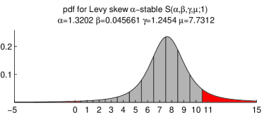
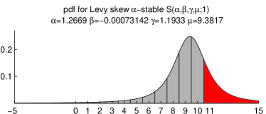
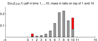
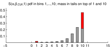
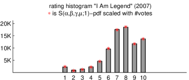
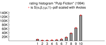
Figure 1: Explanation of confined Lévy skew $\alpha$-stable distributions transformed to rating histograms. Shown are best fits for two examples movies.

The question is now: What is this distribution and how universal can it be parameterised? Before trying to answer this question by looking at the data we formulate a simple social theory which limits the possible distributions to ’Gaussian-like’ shapes.

It is natural to assume that people make their mind about a movie not independent of the opinions of others. Each cinemagoer might adjust her initial impression towards the opinions of others, towards the existing mean rating or towards ratings of professional critics. This is modelled by taking an average of several opinions as the final opinion of a cinemagoer. Here, several aspects might be important like social networks including correlations of links and initial impressions, opinion leaders, timing effects and so on. But if we assume that initial impressions are drawn from a random variable with finite variance, averaging of a large enough number of opinions implies a distribution of averaged opinions close to a normal distribution due to the central limit theorem. This holds also when individual random variables are different under some additional mild assumptions. Also for contrasting forces like ’if I observe the average to be $1\bigstar$ higher then my opinion, I lower my opinion $1\bigstar$’ the limit theorem holds, as long as the forces are linear. According to this theory of opinion making the histogram of ratings should be a discretised and confined probability density function of a normal distribution. The normal distribution does not fit well, as it will turn out. Either the highest peak is not achieved or the decay of bin size with distance from the highest peak is too fast.

Alternatively, we might assume, that initial impressions are drawn from fat-tailed distributions. This implies that distributions do not have a finite variance. The probability of extreme initial impressions might not vanish exponentially but as a power law with exponent $-(1+\alpha)$. If this is the case a generalisation of the central limit theorem says that an average of these random variables has a distribution close to a Lévy skew $\alpha$-stable distribution (the parameter $\alpha$ must indeed be universal for this theorem). So, we can keep the theory of averaging, but extend from the normal distribution to the wider class of Lévy skew $\alpha$-stable distributions.

The Lévy skew alpha-stable distributions are the only stable distributions (see Nolan2010StableDistributions ). It has four parameters $\alpha,\beta,\gamma,\mu$ and is abbreviated $S(\alpha,\beta,\gamma,\mu)$. (There are several parametrisations of the Lévy skew $\alpha$-stable distribution. The one used here is $S(\alpha,\beta,\gamma,\mu;1)$ as explained in Nolan2010StableDistributions .) Its probability density function is

$$f_{S(\alpha,\beta,\gamma,\mu)}(x)=\frac{1}{2\pi}\int_{-\infty}^{+\infty}\varphi(t;\alpha,\beta,\gamma,\mu)e^{-itx}\,dt$$ (1)

with $\varphi(t;\alpha,\beta,\gamma,\mu)$ being its characteristic function given by

$$\varphi(t;\alpha,\beta,\gamma,\mu)=\exp\left[\mu\!-\!|\gamma t|^{\alpha}\,(1\!-\!i\beta\,\textrm{sign}(t)\Phi)~{}\right].$$ (2)

and $\Phi=\tan(\frac{\pi\alpha}{2})$ if $\alpha\neq 1$ and $\Phi=-\frac{2}{\pi}\log|t|$. The four parameters are $\alpha\in]0,2]$, , $\beta[-1,1]$, $\gamma\in[0,\infty[$, and $\mu\in]-\infty,\infty[$. The first two parameters are shape parameters, where $\alpha$ represents the peakedness and $\beta$ the skewness; $\mu$ and $\gamma$ are location and scale parameters. (But notice that $\beta$ is not the skewness in terms of the third moment, and $\alpha$ is not the peakedness in terms of kurtosis.) For $\alpha>1$, $\mu$ also represents the mean of the distribution (otherwise not defined). Figure 2 shows how the parameters modify the shape of the probability density function.

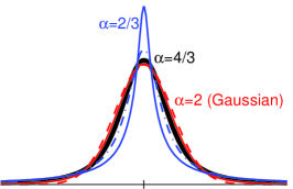
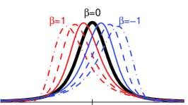
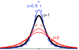
Figure 2: Role of parameters $\alpha,\beta,\gamma$ for the shape of the probability density function of Lévy skew $\alpha$-stable distributions. The base line case in black is the probability density function of $S(\frac{4}{3},0,1,\mu)$ with mu marked on the x-axis.

Small $\alpha$ represents a sharp peak but heavy tails which asymptotically decay as power laws with exponent $-(\alpha+1)$. Maximal $\alpha=2$ is the normal distribution with exponential decay at the tails. Scale parameter $\gamma$ corresponds to the variance $\sigma^{2}$ by the relation $\sigma^{2}=2\gamma^{2}$ only for $\alpha=2$. For lower $\alpha$ the variance is infinite. Skewness $\beta=0$ gives a distribution symmetric around the mean, a positive $\beta$ implies a heavier left tail, a negative $\beta$ a heavier right tail, but with the same decay on both sides. Only in the case $\beta=\pm 1$ one tail vanishes completely. If $\alpha=2$ then $\beta$ has no effect. Only the special cases of the normal distribution ($S(2,0,\sigma,\mu)$), the Cauchy distribution ($S(1,0,\gamma,\delta)$) and the Lévy distribution ($S(\frac{1}{2},1,\gamma,\delta)$) have closed form expressions.

In the following the Lévy skew $\alpha$-stable distributions (discretised and confined) will be fitted for each empirical rating distributions in the data set.

3 Fitted Lévy skew $\alpha$-stable distributions

Fitting is done by minimising least squares of the difference of the normalised empirical rating histogram to the confined and discretised probability density function of Lévy skew $\alpha$-stable distributions with parameters $(\alpha,\beta,\gamma,\mu)$. (For numerical reasons, fitting has been done with a different parameterisation $S(\alpha,\beta,\gamma,\delta;0)$ (see Nolan2010StableDistributions ). The parameters $\alpha,\beta,\gamma$ are equal to the former parameterisation and $\mu=\delta-\beta\gamma\tan(\pi\alpha/2)$.) Computation was performed as follows: The values of the probability density function $f_{S(\alpha,\beta,\gamma,\mu)}(x)$ are computed for $x=-20,-19,\dots,29,30$ by computing and integrating the characteristic function (Eq. 2) on $t=-20.005,\stackrel{{\scriptstyle+0.01}}{{\dots}}:20.005$. Then values for $x=-20,\dots,1$ are summed up and set on bin 1 and values for $x=10,\dots,30$ are summed up and set on bin 10. This produces a probability mass function on $1,\dots,10$ for $(\alpha,\beta,\gamma,\mu)$. Results were reasonably good, the missing mass of the tails (below -20 and above +30) was mostly below $0.3\%$. The fitting was computed by minimising the squares of distances of the probability mass function for $S(\alpha,\beta,\gamma,\mu)$ to the normalised empirical rating distribution. The minima were found with the matlab-function fminsearch. The search converged in $1081$ cases ($99.5\%$) the remaining cases it terminated by maximum number of iterations. Finding a global minimum is not guaranteed by this method, but results looked convincing. (Experimentally, some fits have been computed via minimising by gradient descent. It lead to very similar fits.) We refer to this fit as $\textrm{fit}(\alpha,\beta,\gamma,\mu)$ Examples of fits are shown in Figure 1.

Table 1 shows the mean values of fitted parameters over all movies as well as goodness-of-fit measures. The sum of squared error ($\textrm{SSE}=\sum_{i=1}^{10}(r_{i}-f_{S(\alpha,\beta,\gamma,\mu)}(i))^{2}$ with $r_{i}$ being the fraction of ratings for $i\bigstar$) is on average very small, the coefficient of determination $R^{2}$ is on average almost one. ($R^{2}=1-\frac{\textrm{SSE}}{\sum_{i=1}^{10}(r_{i}-\left\langle r\right\rangle)}$ with $r_{i}$ the fraction of ratings for $i\bigstar$ (therefore $\left\langle r\right\rangle=0.1$).) Both reflects that indeed most fits also look impressively close to the empirical histogram. Further on, a Kolmogorov-Smirnov test has been performed for each movie. (Done with the matlab-function kstest2 on the vector of all ratings and a vector with the same number of ratings as expected according to the fit.) With level of significance $0.05$ the null hypothesis that the expected fitted distribution and the empirical histogram are drawn from the same distribution could not be rejected for $68.7\%$ of the movies. The Kolmogorov-Smirnov test is very hard, it rejects the null hypothesis very likely for large samplesizes. Given the high number of ratings ($>20,000$) for each movie this rate is still impressive. But it is also clear that Lévy skew $\alpha$-stable cannot fully explain all possible rating histograms.

For comparison Table 1 also contains mean values for a fit with normal distributions $S(2,0,\gamma,\mu)$. The goodness-of-fit parameters are worse. This is natural because there are less free parameters, but clearly the normal distribution is ruled out as an appropriate candidate.

	$\left\langle\textrm{ratings}\right\rangle$	corr-coef	$\left\langle\textrm{fit}(\alpha,\beta,\gamma,\mu)\right\rangle$	$\left\langle\textrm{fit}(2,0,\gamma,\mu)\right\rangle$	$\left\langle\textrm{fit}(\mu)\right\rangle$
mean	7.3464	0.5772	7.6326	7.6590	7.5862	$\mu$
std	1.9669	0.8883	1.2021	1.2456	1.1993	$\gamma$
skewness	-1.0610	-0.2829	0.0159	0	-0.0114	$\beta$
kurtosis	1.8581	-0.0138	1.3261	2	$\frac{4}{3}$	$\alpha$
			0.0002	0.0035	0.0035	SSE
			0.9965	0.9404	0.9434	$R^{2}$
			68.7%	0%	4.5%	K-S $\checkmark$

Table 1: Aggregated measures on the data set and on three confined Lévy skew $\alpha$-stable fits ($\textrm{fit}(\alpha,\beta,\gamma,\mu)$, $\textrm{fit}(2,0,\gamma,\mu)$, $\textrm{fit}(\mu)$). Mean, standard deviation, skewness, and kurtosis are computed for the histograms of each movie. Parameters of fits are also computed for each movie. The table shows the mean values for all 1,086 movies. The correlation coefficient is computed for the ‘analog’ measures for the ratings and $\textrm{fit}(\alpha,\beta,\gamma,\mu)$. The low (and negative) correlation skewness vs. $\beta$ and kurtosis vs. $\alpha$ show that the parameters of the fit deliver information on the distribution which is not extracted by the ‘standard measures’ on the raw data. Goodness-of-fit parameter are computed for each fit for each movie. The mean over all movies is shown for sum of squared error (SSE) and coefficient of determination R-square. For the Kolomogorov-Smirnov test (K-S) the rate of not rejecting of the hypothesis of a common distribution of ratings and fitted distribution is given.

Figure 3 shows the parameters of best fits for all movies as scatter plots. All four subplots show $\mu$ at the abscissa. Dark points indicate movies which fits have a small sum of squared errors (SSE), red stars indicate medium SSE, and yellow stars indicate bad fits with high SSE.

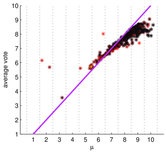
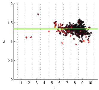
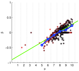
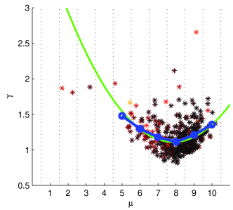
Figure 3: Parameters of best fit for confined Levy skew $\alpha$-stable distributions for all movies. $\mu$ is the mean of the distribution, $\alpha$ modifies peakedness and tail exponent, $\beta$ skewness, and $\gamma$ scales how broad the distribution is.

The first plot shows $\mu$ with respect to the original average of ratings. It shows that $\mu$ is spread wider than the original average. So, $\mu$ can serve as a measure for movie quality which differentiates better than the original average.

The remaining three subplots show the relations of $\mu$ to the other three parameters $\alpha,\beta,\gamma$ of the best Lévy skew $\alpha$-stable fits. The blue dots in the two bottom plots show the averages of the ordinate values within the $\mu$-region marked by the grid lines. The green lines represents $\alpha=\frac{4}{3}$, for $\beta$ the best linear fit for the blue dots, and the best quadratic fit for $\gamma$. The plots show that the peakedness $\alpha$ concentrates to values between $1.2$ and $1.5$, which is clearly not normal distributed. The average value is $\left\langle\alpha\right\rangle=1.3261\approx\frac{4}{3}$. For the skewness $\beta$ there is a clear trend with respect to $\mu$. Interestingly, $\beta=0$ is most likely almost exactly at $\mu=7.6326$ which is equal to $\left\langle\mu\right\rangle$. For better movies there is an additional positive skewness (meaning that the right tail is fatter). Respectively, for movies worse than $\left\langle\mu\right\rangle$ there is additional negative skewness (meaning that the left tail is fatter). For the scale parameter there is also a clear trend visible. The most narrow distribution is achieved also almost exactly for movies with $\mu=\left\langle\mu\right\rangle$. For better and worse movies the distributions get broader.

It is not apriori clear and thus remarkable that $\left\langle\mu\right\rangle$ plays a central role for the deviations in $\beta$ and $\gamma$ with respect to $\mu$. This gives rise to the speculation that $\left\langle\mu\right\rangle$ is kind of universal modulo the scale of ratings (here $1,\dots,10$). This is underpinned by the finding of Cosley.Lam.ea2003Isseeingbelieving that users rate consistently in different rating schemes. If we rescale $\left\langle\mu\right\rangle=7.6326$ to the scale $1,\dots,5$ we get $4.0633$ which coincides almost exactly with $4.07$ which is the average mean rating of books averaged over all books in the amazon.com-sample of Li.Hitt2004SelfSelectionand . Rescale is done under the assumption that each rating stands for a bin centred on the rating with width equal to the distance of successive ratings (here 1). Thus a $10\bigstar$-rating $r_{10}$ is converted to the 5$\bigstar$-rating by $r_{5}=5(\frac{r_{10}-0.5}{10})+0.5$. This ensures for examples that $1\bigstar$ in a $5\bigstar$-rating corresponds to $1.5\bigstar$ stars in a 10$\bigstar$-rating, respectively $5\bigstar$ corresponds to $9.5\bigstar$. It does not coincide as good with $3.44$ which was found by Dellarocas.Narayan2006StatisticalMeasureof for movies.yahoo.com-data. The deviation may come from two differences: First, in Li.Hitt2004SelfSelectionand and in this study the average reported is the average of the average ratings of movies, while Dellarocas.Narayan2006StatisticalMeasureof reports the the pure average rating over all ratings in the database. Second, Li.Hitt2004SelfSelectionand and this study select books respectively movies similar: this study by all having more than 20,000 ratings, and Li.Hitt2004SelfSelectionand by being on a bestseller list and having a sufficient number of reviews. Both sampling method imply a similar selection bias which is different from Dellarocas2003DigitizationofWord which collects all movies released in 2002.

Taking this speculation as true it means that an average movie receives an average vote of about $0.71$ on a generalised scale $[0,1]$. This indicates a universal strong positive bias for the average movie. The strong positive bias may be implied by an overall selection-bias, that user select movies or products they are likely to like or even they like movies and products just because they paid for them. Contrasting, a negative bias is reported on ratings for jokes in Goldberg.Roeder.ea2001EigentasteConstantTime . Following the results of $\textrm{fit}(\alpha,\beta,\gamma,\mu)$ we further conclude that the distribution of ratings for an average movie has no skewness ($\beta=0$) and the smallest scale parameter (here $\gamma=1.1$). If a movie deviates from average this implies higher deviations in the distribution ($\gamma>1.1$) and a skewness which pronounces the deviation from the average movie. The latter observation can be regarded as a hint for a socially implied positive feedback in determining opinions on movies which quality is above (or below) an average movie.

Taking the trends displayed by the green lines in Figure 3 one can construct a one-parameter fit on $\mu$ with $\alpha=\frac{4}{3}$, $\beta$ determined by the linear fit and $\gamma$ by the quadratic fit. The equations to compute $\beta,\gamma$ from $\mu$ are $\beta=b_{1}\mu+b_{2}$ and $\gamma=c_{1}\mu^{2}+c_{2}\mu+c_{3}$ with parameters $b_{1}=0.1178,b_{2}=-0.9049,c_{1}=0.05342,c_{2}=-0.8388,c_{3}=4.401$. We refer to this fit as $\textrm{fit}(\mu)$. Mean values and mean goodness-of-fit measures are also shown in Table 1. The one-parameter fit gets better goodness than the two parameter $\textrm{fit}(2,0,\gamma,\mu)$.

Figure 4 shows how $\textrm{fit}(\mu)$ is able to approximate empirical histograms. The shape of empirical distributions is well captured but variations for different movies are big enough to conclude that $\textrm{fit}(\mu)$ can only be seen as a baseline case. Movies can have some individual characteristics of their rating distribution which go beyond the quality (captured in $\mu$). Deviations from the baseline case can be used to classify movies in a new way to understand what the cause of deviations might be. This is a task for further research.

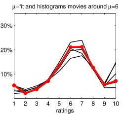
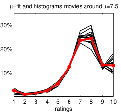
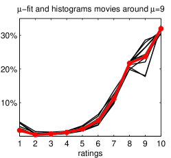
Figure 4: The theoretical probability mass functions according to the parameters of $\textrm{fit}(\mu)$ for $\mu=6,7.5,9$ and all empirical histograms which received best fitted values for $\mu\in[5.98,6.02],[7.48,7.52],[8.98,9.02]$.

Finally, Figure 5 shows a comparison of theoretical histograms of $\textrm{fit}(\mu)$ and the average empirical histograms. The theoretical histograms are for $\mu=5,\stackrel{{\scriptstyle+0.5}}{{\dots}},9$ and the average empirical histograms are over all movies with fitted value of $\mu$ within the intervals $\mu\in[4.75,5.25]$, $[5.25,5.75]$, $\dots$, $[8.25,8.75]$, $[8.75,9.25]$. The similarity underpins that $\textrm{fit}(\mu)$ can really serve as a good baseline case. But some deviations from the baseline case seem to be not totally random. E.g. the residuals show that the size of the $1\bigstar$ bin for low quality movies ($\mu<7$) is on average predicted too high, while the $2\bigstar,3\bigstar$ bins are on average predicted too low.

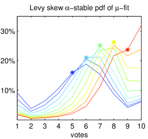
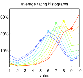
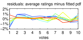
Figure 5: The theoretical probability mass functions according to the parameters of $\textrm{fit}(\mu)$ for $\mu=5,\stackrel{{\scriptstyle+0.5}}{{\dots}},9$ (left), empirical average histograms for all movies with best fitted values for $\mu\in[4.75,5.25]$, $[5.25,5.75]$,$\dots$, $[8.25,8.75]$, $[8.75,9.25]$ (right), and residuals of both. The stars mark the underlying $\mu$-values of curves. Colors are the same in all plots.

4 Conclusion

With some success rating histograms were fitted to confined Lévy skew $\alpha$-stable distributions. This clearly demonstrates that the assumptions that opinions are normally distributed, beta distributed or U-shaped around the quality of the movie is not valid. Some histograms have of course a U-shaped (or better J-shaped) form, e.g. right-hand side in Figure 1. But a U-shape can not approxiamte all histograms, e.g. left-hand side of Figure 1.

If the assumption that expressed opinions of users are weighted averages of formerly expressed opinions of others this implies that these opinions must come from distributions with fat tails with a power-law exponent of about $1.2$ to $1.5$ to get good fits. Further on, the scale and skewness parameter of the best fits change systematically with the deviation of its mean from the mean of an average movie (with $\mu\approx 7.6$). A movie better than average shows right skewness and a larger scale parameter. A movie worse than average shows left skewness and a also a larger scale parameter. Thus, better movies have also a heavier tail on the better side and worse movies have a heavier tail on the worse side. In general, distributions get broader when deviating from the mean. Both observations seem plausible from a sociological point of view. The new measures of skewness ($\beta$) and peakedness ($\alpha$) are not the same as the classical skewness and excess kurtosis which are compute directly from the sample data (see Table 1). There is no correlation of both measures, or even a negative one. This underpins, that fitting rating histograms as confined distributions really delivers a new characterisation. A further advantage of this approach is, that the Lévy skew $\alpha$-stable distribution defines a distribution completely, which mean, standard deviation, skewness and excess kurtosis do not.

A one-parameter fit based on this observations shows to approximate the data well, but is not able to establish a strict characterisation of movie histograms. Deviations from the constructed baseline case are not neglectable. Nevertheless, it could be useful to characterise movies by their deviation from their baseline case. Further on, there might is a selection bias in the data, because only movies with a large number of ratings were selected. The fit might not work for less rated movies. The method might be used to detect attacks of enthusiastic fans (or movie companies) which try to rate movies up.

There seems to be some universality in movie rating distributions, which may be implied by people adjusting their opinions with peers and other sources of opinions. Clearly, other theories which may imply other underlying distributions need to be developed and checked against data and also this theory needs to be checked against data from other sources to clarify universality in continuous opinion dynamics about taste.

Acknowledgement

The research leading to these results has received funding from the European Community’s Seventh Framework Programme (FP7/2007-2013) under grant agreement no. 231323 (CyberEmotions project).

References

- (1) S. Asch, Scientific American 193(5), 31 (1955)
- (2) I. Lorge, D. Fox, J. Davitz, M. Brenner, Psychological Bulletin 55(6), 337 (1958)
- (3) M. Sherif, C. Hovland, Social Judgment: Assimilation and Contrast Effects in Communication and Attitude Change (Yale University Press, New Haven, CT, 1961)
- (4) J. Forgas, European Journal of Social Psychology 7(2), 175 (1977)
- (5) N. Friedkin, American Sociological Review 64(6), 856 (1999)
- (6) M. Salganik, P. Dodds, D. Watts, Science 311(5762), 854 (2006)
- (7) W. Mason, F. Conrey, E. Smith, Personality and Social Psychology Review 11(3), 279 (2007)
- (8) G. Deffuant, D. Neau, F. Amblard, G. Weisbuch, Advances in Complex Systems 3, 87 (2000)
- (9) R. Hegselmann, U. Krause, Journal of Artificial Societies and Social Simulation 5(3), 2 (2002), http://jasss.soc.surrey.ac.uk/5/3/2.html
- (10) D. Urbig, Journal of Artificial Societies and Social Simulation 6(1), 2 (2003), http://www.jasss.surrey.ac.uk/6/1/2.html
- (11) G. Deffuant, D. Neau, F. Amblard, G. Weisbuch, Journal of Artificial Societies and Social Simulation 5(4) (2002)
- (12) W. Jager, F. Amblard, Computational & Mathematical Organization Theory 10, 295 (2004)
- (13) L. Salzarulo, Journal of Artificial Societies and Social Simulation 9(1), 13 (2006), http://jasss.soc.surrey.ac.uk/9/1/13.html
- (14) D. Baldassarri, P. Bearman, American Sociological Review 72(5), 784 (2007)
- (15) D. Stauffer, AIP Conference Proceedings 779, 56 (2005)
- (16) J. Lorenz, Int. Journal of Modern Physics C 18(12), 1819 (2007)
- (17) C. Castellano, S. Fortunato, V. Loreto, Review of Modern Physics 81, 591 (2009)
- (18) D. Turnbull, in CHI ’07: CHI ’07 extended abstracts on Human factors in computing systems (ACM, 2007), pp. 2705–2710
- (19) J. Lorenz, in Managing Complexity: Insights, Concepts, Applications, edited by D. Helbing (Springer, 2008)
- (20) C. Dellarocas, Management Science 49(10), 1407 (2003)
- (21) K. Goldberg, T. Roeder, D. Gupta, C. Perkins, Information Retrieval 4(2), 133 (2001)
- (22) K. Cheung, J. Kwok, M. Law, K. Tsui, Decision Support Systems 35(2), 231 (2003)
- (23) A. Umyarov, A. Tuzhilin, Leveraging aggregate ratings for better recommendations, in RecSys ’07: Proceedings of the 2007 ACM conference on Recommender systems (ACM, 2007), pp. 161–164
- (24) D.M. Chance, E. Hillebrand, J.E. Hilliard, Management Science 54(5), 1015 (2008)
- (25) B.J. Jiang, P.Y. Chen, SSRN eLibrary (2007)
- (26) D. Cosley, S. Lam, I. Albert, J. Konstan, J. Riedl, Proceedings of the SIGCHI conference on Human factors in computing systems pp. 585–592 (2003)
- (27) X. Li, L.M. Hitt, Information Systems Research 19(4), 456 (2008)
- (28) F. Wu, B.A. Huberman, Arxiv preprint arXiv: 0805.3537 (2008)
- (29) C. Dellarocas, R. Narayan, Statistical Science 21(2), 277 (2006)
- (30) C. Borghesi, J.P. Bouchaud, Quality and Quantity 41(4), 557 (2007)
- (31) B. Gu, M. Lin, The Dynamics of Online Consumer Reviews, in Workshop on Information Systems and Economics (WISE) (2006)
- (32) I looked at all movies with more than ratings on IMDb.com in March 2008. These were identified by IMDb “Power Search”-function. These were histograms.
- (33) J.P. Nolan, Stable Distributions - Models for Heavy Tailed Data (Birkhäuser, 2010), in progress, Chapter 1 online at academic2.american.edu/jpnolan