Fractional dynamic symmetries and the ground state properties of nuclei

Abstract

Based on the Riemann- and Caputo definition of the fractional derivative we use the fractional extensions of the standard rotation group $SO(3)$ to construct a higher dimensional representation of a fractional rotation group with mixed derivative types. An extended symmetric rotor model is derived, which predicts the sequence of magic proton and neutron numbers accurately. The ground state properties of nuclei are correctly reproduced within the framework of this model.

1 Introduction

The experimental evidence for discontinuities in the sequence of atomic masses, $\alpha-$ and $\beta$- decay systematics and binding energies of nuclei suggests the existence of a set of magic proton and neutron numbers, which can be described successfully by single particle shell models with a heuristic spin-orbit term [1], [2]. The most prominent representative is the phenomenological Nilsson model [3] with an anisotropic oscillator potential:

$$V(x_{i})=\sum_{i=1}^{3}{1\over 2}m\omega_{i}^{2}x_{i}^{2}-\hbar\omega_{0}\kappa(2\vec{l}\vec{s}+\mu l^{2})$$ (1)

Although these models are flexible enough to reproduce the experimental results, they lack a deeper theoretical justification, which becomes obvious, when extrapolating the parameters $\kappa$, $\mu$, which determine the strength of the spin orbit and $l^{2}$ term to the region of superheavy elements [5].

Hence it seems tempting to describe the experimental data with alternative methods. Typical examples are relativistic mean field theories [6],[7], where nucleons are described by the Dirac-equation and the interaction is mediated by mesons. Although a spin orbit force is obsolete in these models, different parametrizations predict different shell closures [8],[9]. Therefore the problem of a theoretical foundation of magic numbers remains an open question since Elsasser [10] raised the problem 75 years ago.

A fundamental understanding of magic numbers for protons and neutrons may be achieved if the underlying corresponding symmetry of the nuclear many body system is determined. Therefore a group theoretical approach seems appropriate.

Group theoretical methods have been successfully applied to problems in nuclear physics for decades. Elliott [11] has demonstrated, that an average nuclear potential given by a three dimensional harmonic oscillator corresponds to a SU(3) symmetry. Low lying collective states have been successfully described within the IBM-model [12], which contains as one limit the five dimensional harmonic oscillator, which is directly related to the Bohr-Mottelson Hamiltonian.

In this paper we will determine the symmetry group, which generates a single particle spectrum similar to (1), but includes the magic numbers right from the beginning.

Our approach is based on group theoretical methods developed within the framework of fractional calculus.

The fractional calculus [13]-[16] provides a set of axioms and methods to extend the coordinate and corresponding derivative definitions in a reasonable way from integer order n to arbitrary order $\alpha$:

$$\{x^{n},{\partial^{n}\over\partial x^{n}}\}\rightarrow\{x^{\alpha},{\partial^{\alpha}\over\partial x^{\alpha}}\}$$ (2)

The definition of the fractional order derivative is not unique, several definitions e.g. the Feller, Fourier, Riemann, Caputo, Weyl, Riesz, Grünwald fractional derivative definitions coexist [17]-[25]. A direct consequence of this diversity is the fact, that the solutions e.g. of a one dimensional wave equation differ significantly depending on the specific choice of a fractional derivative definition.

Until now it has always been assumed, that the fractional derivative type for an extension of a fractional differential equation to multi-dimensional space should be chosen uniquely.

In contrast to this assumption, in this paper we will investigate properties of higher dimensional rotation groups with mixed Caputo and Riemann type definition of the fractional derivative. We will demonstrate, that a fundamental dynamic symmetry is established, which determines the magic numbers for protons and neutron respectively and furthermore describes the ground state properties of nuclei with reasonable accuracy.

2 Notation

We will investigate the spectrum of multi dimensional fractional rotation groups for two different definitions of the fractional derivative, namely the Riemann- and Caputo fractional derivative. Both types are strongly related.

Starting with the definition of the fractional Riemann integral

$${{}_{\textrm{\tiny{R}}}}I^{\alpha}\,f(x)=\cases{({{}_{\textrm{\tiny{R}}}}I_{+}^{\alpha}f)(x)=\frac{1}{\Gamma(\alpha)}\int_{0}^{x}d\xi\,(x-\xi)^{\alpha-1}f(\xi)&\qquad\, $x\geq 0$\\ ({{}_{\textrm{\tiny{R}}}}I_{-}^{\alpha}f)(x)=\frac{1}{\Gamma(\alpha)}\int_{x}^{0}d\xi\,(\xi-x)^{\alpha-1}f(\xi)&\qquad\, $x<0$\\ }$$ (3)

where $\Gamma(z)$ denotes the Euler $\Gamma$-function, the fractional Riemann derivative is defined as the product of a fractional integration followed by an ordinary differentiation:

$${{}_{\textrm{\tiny{R}}}}\partial_{x}^{\alpha}=\frac{\partial}{\partial x}{{}_{\textrm{\tiny{R}}}}I^{1-\alpha}$$ (4)

It is explicitely given by:

$${{}_{\textrm{\tiny{R}}}}\partial_{x}^{\alpha}\,f(x)=\cases{({{}_{\textrm{\tiny{R}}}}\partial_{+}^{\alpha}f)(x)=\frac{1}{\Gamma(1-\alpha)}\frac{\partial}{\partial x}\int_{0}^{x}d\xi\,(x-\xi)^{-\alpha}f(\xi)&$x\geq 0$\\ ({{}_{\textrm{\tiny{R}}}}\partial_{-}^{\alpha}f)(x)=\frac{1}{\Gamma(1-\alpha)}\frac{\partial}{\partial x}\int_{x}^{0}d\xi\,(\xi-x)^{-\alpha}f(\xi)&$x<0$\\ }$$ (5)

The Caputo definition of a fractional derivative follows an inverted sequence of operations (4). An ordinary differentiation is followed by a fractional integration

$${{}_{\textrm{\tiny{C}}}}\partial_{x}^{\alpha}={{}_{\textrm{\tiny{R}}}}I^{1-\alpha}\frac{\partial}{\partial x}$$ (6)

which results in:

$${{}_{\textrm{\tiny{C}}}}\partial_{x}^{\alpha}\,f(x)=\cases{({{}_{\textrm{\tiny{C}}}}\partial_{+}^{\alpha}f)(x)=\frac{1}{\Gamma(1-\alpha)}\int_{0}^{x}d\xi\,(x-\xi)^{-\alpha}\frac{\partial}{\partial\xi}f(\xi)&$x\geq 0$\\ ({{}_{\textrm{\tiny{C}}}}\partial_{-}^{\alpha}f)(x)=\frac{1}{\Gamma(1-\alpha)}\int_{x}^{0}d\xi\,(\xi-x)^{-\alpha}\frac{\partial}{\partial\xi}f(\xi)&$x<0$\\ }$$ (7)

Applied to a function set $f(x)=x^{n\alpha}$ using the Riemann fractional derivative definition (5) we obtain:

$${{}_{\textrm{\tiny{R}}}}\partial_{x}^{\alpha}\,x^{n\alpha} = \frac{\Gamma(1+n\alpha)}{\Gamma(1+(n-1)\alpha)}\,x^{(n-1)\alpha}$$ (8)

$$= {{}_{\textrm{\tiny{R}}}}[n]\,x^{(n-1)\alpha}$$ (9)

where we have introduced the abbreviation ${{}_{\textrm{\tiny{R}}}}[n]$.

For the Caputo definition of the fractional derivative it follows for the same function set:

$${{}_{\textrm{\tiny{C}}}}\partial_{x}^{\alpha}\,x^{n\alpha} = \cases{\frac{\Gamma(1+n\alpha)}{\Gamma(1+(n-1)\alpha)}\,x^{(n-1)\alpha}&$n>0$\\ 0&$n=0$\\ }$$ (10)

$$= {{}_{\textrm{\tiny{C}}}}[n]\,x^{(n-1)\alpha}$$ (11)

where we have introduced the abbreviation ${{}_{\textrm{\tiny{C}}}}[n]$.

Both derivative definitions only differ in the case $n=0$:

$${{}_{\textrm{\tiny{C}}}}[n] = {{}_{\textrm{\tiny{R}}}}[n]-\delta_{n0}\,{{}_{\textrm{\tiny{R}}}}[0]$$ (12)

$$= {{}_{\textrm{\tiny{R}}}}[n]-\delta_{n0}\,\frac{1}{\Gamma(1-\alpha)}$$ (13)

where $\delta_{mn}$ denotes the Kronecker-$\delta$. We will rewrite equations (9) and (11) simultaneously, introducing the short hand notation

$${{}_{\textrm{\tiny{R,C}}}}\partial_{x}^{\alpha}\,x^{n\alpha}={{}_{\textrm{\tiny{R,C}}}}[n]\,x^{(n-1)\alpha}\\$$ (14)

We now introduce the fractional angular momentum operators or generators of infinitesimal rotations in the $i,j$ plane on the $N$-dimensional Euclidean space:

$${{}_{\textrm{\tiny{R,C}}}}L_{ij}(\alpha)={{}_{\textrm{\tiny{R,C}}}}\,i\hbar(x_{i}^{\alpha}\partial_{j}^{\alpha}-x_{j}^{\alpha}\partial_{i}^{\alpha})$$ (15)

The commutation relations of the fractional angular momentum operators are isomorph to the fractional extension of the rotational group $SO(N)$

$${{}_{\textrm{\tiny{R,C}}}}\,[L_{ij}(\alpha),L_{kl}(\alpha)] = {{}_{\textrm{\tiny{R,C}}}}\,i\hbar{f_{ijkl}}^{mn}L_{mn}(\alpha)$$

$$\qquad\qquad\qquad i,j,k,l,m,n=1,2,..,N$$

with structure coefficients ${{}_{\textrm{\tiny{R,C}}}}{f_{ijkl}}^{mn}$. Their explicit form depends on the function set the fractional angular momentum operators act on and on the fractional derivative type used.

The Casimir-operators of the fractional rotation group ${{}_{\textrm{\tiny{R}}}}SO^{\alpha}(3)$ based on the Riemann fractional derivative definition have been derived in [26] and for ${{}_{\textrm{\tiny{C}}}}SO^{\alpha}(3)$ based on the Caputo fractional derivative definition are given in [27]. We summarize the major results:

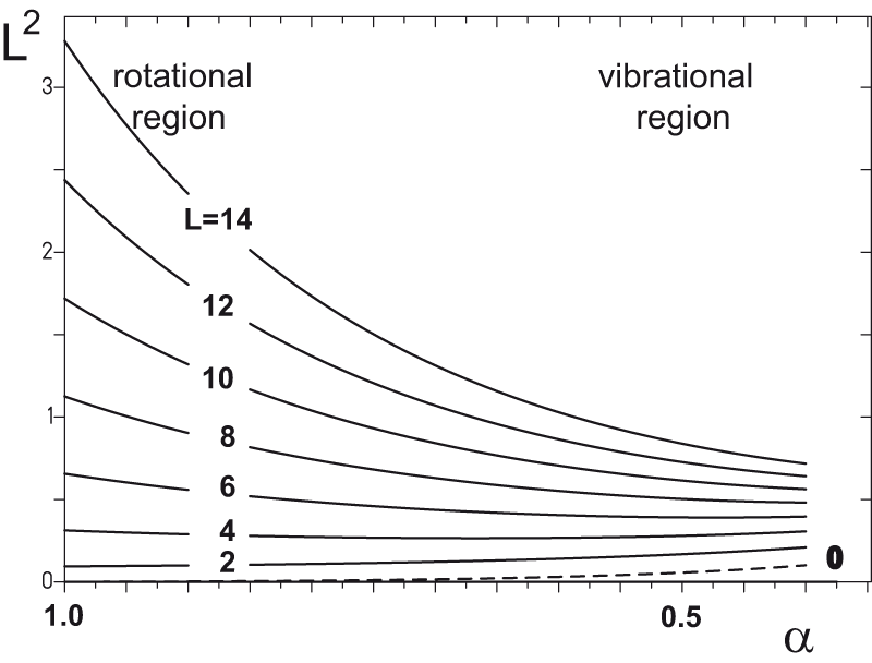
Figure 1: Spectrum of the Casimir operator $L^{2}(L,\alpha)$ from (2) as a function of the fractional derivative coefficient $\alpha$. Only the $L=0$ state differs for Riemann and Caputo derivative.

According to the group chain

$${{}_{\textrm{\tiny{R,C}}}}SO^{\alpha}(3)\supset{{}_{\textrm{\tiny{R,C}}}}SO^{\alpha}(2)$$ (17)

there are two Casimir-operators $\Lambda_{i}$, namely $\Lambda_{2}=L_{z}(\alpha)=L_{12}(\alpha)$ and $\Lambda_{3}=L^{2}(\alpha)=L_{12}^{2}(\alpha)+L_{13}^{2}(\alpha)+L_{23}^{2}(\alpha)$. We introduce the two quantum numbers $L$ and $M$, which completely determine the eigenfunctions $|LM>$. It follows

$${{}_{\textrm{\tiny{R,C}}}}\,L_{z}(\alpha)|LM> = {{}_{\textrm{\tiny{R,C}}}}\,\hbar\,\textrm{sign}(M)\,[|M|]\,|LM>$$

$$\qquad\qquad\qquad M=-L,-L+1,...,\pm 0,...,L$$

$${{}_{\textrm{\tiny{R,C}}}}\,L^{2}(\alpha)|LM> = {{}_{\textrm{\tiny{R,C}}}}\,\hbar^{2}[L][L+1]\,|LM>$$

$$\qquad\qquad\qquad L=0,1,2,...$$

where $|M|$ denotes the absolute value of $M$. In addition, on the set of eigenfunctions $|LM>$, the parity operator $\Pi$ is diagonal and has the eigenvalues

$$\Pi|LM>=(-1)^{L}|LM>$$ (20)

In figure 1 the eigenvalues of the Casimir-operator $L^{2}$ are shown as a function of $\alpha$. Only in the case $L=0$ the spectra differ for the Riemann- and Caputo derivative. While for the Caputo derivative

$${{}_{\textrm{\tiny{C}}}}\,L^{2}(\alpha)|00>=0$$ (21)

because ${{}_{\textrm{\tiny{C}}}}[0]=0$, using the Riemann derivative for $\alpha\neq 1$ there is a nonvanishing contribution

$${{}_{\textrm{\tiny{R}}}}L^{2}(\alpha)|00>={{}_{\textrm{\tiny{R}}}}\hbar^{2}[0][1]|00>=\hbar^{2}\frac{\Gamma(1+\alpha)}{\Gamma(1-\alpha)}|00>$$ (22)

3 The Caputo-Riemann-Riemann symmetric rotor

We now use group theoretical methods to construct higher dimensional representations of the fractional rotation groups ${{}_{\textrm{\tiny{R,C}}}}SO^{\alpha}(3)$.

As an example of physical relevance we introduce the group ${{}_{\textrm{\tiny{CRR}}}}G$ with the following chain of subalgebras:

$${{}_{\textrm{\tiny{CRR}}}}G\supset{{}_{\textrm{\tiny{C}}}}SO^{\alpha}(3)\supset{{}_{\textrm{\tiny{R}}}}SO^{\alpha}(3)\supset{{}_{\textrm{\tiny{R}}}}SO^{\alpha}(3)$$ (23)

The Hamiltonian $H$ can now be written in terms of the Casimir operators of the algebras appearing in the chain and can be analytically diagonalized in the corresponding basis. The Hamiltonian is:

$$H=\frac{\omega_{1}}{\hbar}{{}_{\textrm{\tiny{C}}}}L_{1}^{2}(\alpha)+\frac{\omega_{2}}{\hbar}{{}_{\textrm{\tiny{R}}}}L_{2}^{2}(\alpha)+\frac{\omega_{3}}{\hbar}{{}_{\textrm{\tiny{R}}}}L_{3}^{2}(\alpha)$$ (24)

with the free parameters $\omega_{1},\omega_{2},\omega_{3}$ and the basis is $|L_{1}M_{1}L_{2}M_{2}L_{3}M_{3}>$. Furthermore, we impose the following symmetries:

First, the wave functions should be invariant under parity transformations, which according to (20) leads to the conditions

$$L_{1}=2n_{1}\quad L_{2}=2n_{2}\quad L_{3}=2n_{3},\quad n_{1},n_{2},n_{3}=0,1,2,3,...$$ (25)

second, we require

$${{}_{\textrm{\tiny{C}}}}L_{z_{1}}(\alpha)|L_{1}M_{1}L_{2}M_{2}L_{3}M_{3}> = {{}_{\textrm{\tiny{C}}}}+\hbar[L_{1}]|L_{1}M_{1}L_{2}M_{2}L_{3}M_{3}>$$ (26)

$${{}_{\textrm{\tiny{R}}}}L_{z_{2}}(\alpha)|L_{1}M_{1}L_{2}M_{2}L_{3}M_{3}> = {{}_{\textrm{\tiny{R}}}}+\hbar[L_{2}]|L_{1}M_{1}L_{2}M_{2}L_{3}M_{3}>$$ (27)

$${{}_{\textrm{\tiny{R}}}}L_{z_{3}}(\alpha)|L_{1}M_{1}L_{2}M_{2}L_{3}M_{3}> = {{}_{\textrm{\tiny{R}}}}+\hbar[L_{3}]|L_{1}M_{1}L_{2}M_{2}L_{3}M_{3}>$$ (28)

which reduces the multiplicity of a given $|2n_{1}M_{1}2n_{2}M_{2}2n_{3}M_{3}>$ set to 1.

With these conditions, the eigenvalues of the Hamiltonian (24) are given as

$$E(\alpha) = \hbar\omega_{1}{{}_{\textrm{\tiny{C}}}}[2n_{1}][2n_{1}+1]+$$ (29)

$$\hbar\omega_{2}{{}_{\textrm{\tiny{R}}}}[2n_{2}][2n_{2}+1]+\hbar\omega_{3}{{}_{\textrm{\tiny{R}}}}[2n_{3}][2n_{3}+1]$$

$$= \sum_{i=1}^{3}\hbar\omega_{i}\frac{\Gamma(1+(2n_{i}+1)\alpha)}{\Gamma(1+(2n_{i}-1)\alpha)}-\delta_{n_{1}0}\hbar\omega_{1}\frac{\Gamma(1+\alpha)}{\Gamma(1-\alpha)}$$

$$\qquad\qquad\qquad\qquad\qquad n_{1},n_{2},n_{3}=0,1,2,..$$

on a basis $|2n_{1}2n_{1}2n_{2}2n_{2}2n_{3}2n_{3}>$.

This is the major result of our derivation. We call this model the Caputo-Riemann-Riemann symmetric rotor. What makes this model remarkable is its behaviour near $\alpha=1/2$.

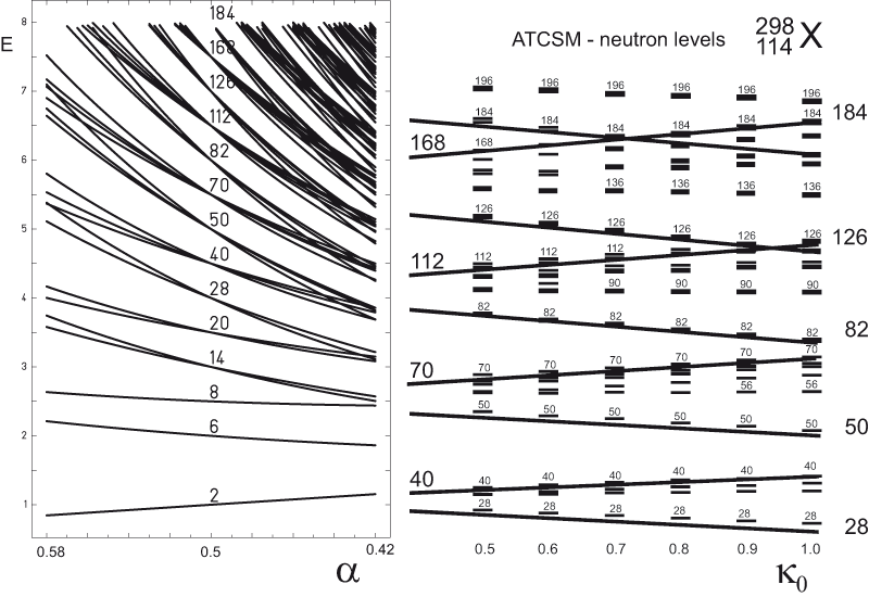
Figure 2: On the left the energy spectrum $E(\alpha)$ from (3) for the spherical case (31) in units of $\hbar\omega_{0}$ for the Caputo-Riemann-Riemann symmetric rotor is presented. The right diagram shows the neutron energy levels for the spherical nucleus ${}^{298}_{114}X$ calculated within the framework of the asymmetric two center shell model (ATCSM) [28] near the ground state as a function of increasing strength of the spin-orbit term ($\kappa_{0}\kappa\vec{l}\vec{s}$) increasing from $50\%$ to $100\%$ of the recommended $\kappa$ value, while the $\mu l^{2}$ value is kept constant. The transition from magic numbers of the standard 3-dimensional harmonic oscillator levels (34) to the shifted set of magic numbers (37) is pointed out with thick lines. Left and right figure therefore show a similar behaviour for the energy levels.

On the left of figure 2 we have plotted the energy levels in the vicinity of $\alpha\approx 1/2$ for the case

$$\omega_{1}=\omega_{2}=\omega_{3}=\omega_{0}$$ (31)

which we denote as the spherical case.

For the idealized case $\alpha=1/2$, using the relation $\Gamma(1+z)=z\Gamma(z)$ the level spectrum (3) is simply given by:

$$E(\alpha=1/2)=\hbar\omega_{0}(n_{1}+n_{2}+n_{3}+\frac{3}{2}-\frac{1}{2}\delta_{n_{1}0})$$ (32)

For $n_{1}\neq 0$ this is the well known spectrum of the 3-dimensional harmonic oscillator. Assuming a twofold spin degeneracy of the energy levels, we introduce the quantum number $N$ as

$$N=n_{1}+n_{2}+n_{3}$$ (33)

Consequently we obtain a first set $n_{\textrm{magic 1}}$ of magic numbers $n_{\textrm{magic}}$

$$n_{\textrm{magic 1}} = \frac{1}{3}(N+1)(N+2)(N+3)\qquad N=1,2,3,...$$ (34)

$$= 8,20,40,70,112,168,240,...$$ (35)

which correspond to the standard 3-dimensional harmonic oscillator at energies

$$E=\hbar\omega_{0}(N+3/2)$$ (36)

In addition, for $n_{1}=0$, which corresponds to the $|00\,2n_{2}2n_{2}\,2n_{3}2n_{3}>$ states, we obtain a second set $n_{\textrm{magic 2}}$ of magic numbers

$$n_{\textrm{magic 2}} = \frac{1}{3}(N+1)(5+(N+1)^{2})\qquad N=0,1,2,3,...$$ (37)

$$= 2,6,14,28,50,82,126,184,258,...$$ (38)

at energies

$$E=\hbar\omega_{0}(N+1)$$ (39)

which is shifted by the amount $-\frac{1}{2}\hbar\omega_{0}$ compared to the standard 3-dimensional harmonic oscillator values.

From figure 2 it follows, that for $\alpha<1/2$ the second set $n_{\textrm{magic 2}}$ of energy levels falls off more rapidly than the levels of set $n_{\textrm{magic 1}}$. As a consequence for decreasing $\alpha$ the magic numbers $n_{\textrm{magic 1}}$ die out successively. On the other hand, for $\alpha>1/2$ the same effect causes the magic numbers $n_{\textrm{magic 1}}$ to survive.

We want to emphasize, that the described behaviour for the energy levels in the region $\alpha<1/2$ may be directly compared to the influence of a $ls$-term in phenomenological shell models. As an example, on the right hand side of figure 2 a sequence of neutron levels for the superheavy element ${}^{298}_{114}X$ calculated with the asymmetric two center shell model (ATCSM) [28] with increasing strength of the $ls$-term from $50\%$ to $100\%$ is plotted. It shows, that the $n=168$ gap breaks down at about $70\%$ and the $n=112$ gap at about $90\%$ of the recommended $\kappa$-value for the $ls$-term. This corresponds to an $\alpha\approx 0.46$ value, since in the Caputo-Riemann-Riemann symmetric rotor the $n=168$ gap breaks down at $\alpha=0.466$, the $n=112$ gap at $\alpha=0.460$ and the $n=70$ gap vanishes at $\alpha=0.453$.

We conclude, that the Caputo-Riemann-Riemann symmetric rotor predicts a well defined set of magic numbers. This set is a direct consequence of the underlying dynamic symmetries of the three fractional rotation groups involved. It is indeed remarkable, that the same set of magic numbers is realized in nature as magic proton and neutron numbers.

In the next section we will demonstrate, that the proposed analytical model is an appropriate tool to describe the ground state properties of nuclei.

4 Ground state properties of nuclei

We will use the Caputo-Riemann-Riemann symmetric rotor (3) as a dynamic shell model for a description of the microscopic part of the total energy $E_{\textrm{tot}}$ of the nucleus.

$$E_{\textrm{tot}} = E_{\textrm{macroscopic}}+E_{\textrm{microscopic}}$$ (40)

$$= E_{\textrm{macroscopic}}+\delta U+\delta P$$ (41)

where $\delta U$ and $\delta P$ denote the shell- and pairing energy contributions.

For the macroscopic contribution we use the finite range liquid drop model (FRLDM) proposed by Möller [31] using the original parameters, except the value for the constant energy contribution $a_{0}$.

As the primary deformation parameter we use the ellipsoidal deformation $Q$:

$$Q={b\over a}={\omega_{3}\over\omega_{1}}={\omega_{3}\over\omega_{2}}$$ (42)

where $a,b$ are the semi-axes of a rotational symmetric ellipsoid. Consequently a value $Q<1$ describes prolate and a value of $Q>1$ descibes oblate shapes. In order to relate the ellipsiodal deformation $Q$ to the quadrupole deformation $\epsilon_{2}$ used by Möller, we define:

$$Q=1-1.43085\epsilon_{2}+0.707669\epsilon_{2}^{2}$$ (43)

Furthermore we extend the original FRLDM-model introducing an additional curvature energy term $V_{R}(Q)$, which describes the interaction of the nucleus with the collective curved coordinate space [32]:

$$V_{R}(Q)=-a_{R}B_{R}A^{-5/3}$$ (44)

where $A$ is the nucleon number, $a_{R}$ is the curvature parameter given in $[{\textrm{MeV}}]$ and the relative curvature energy $B_{R}(Q)$ given as:

$$B_{R}(Q)=9\,Q^{16/3}\left(\frac{199-288\log(2)}{(2+Q^{2})(266-67Q^{2}+96(Q^{2}-4)\log(2))}\right)^{2}$$ (45)

which is normalized relative to a sphere $B_{R}(Q=1)=1$.

Therefore the total energy may be splitted into

$$E_{\textrm{tot}}=E_{\textrm{mac}}+E_{\textrm{mic}}$$ (46)

where

$$E_{\textrm{mac}}(a_{0},a_{R}) = {\textrm{FRLDM}}(a_{0},Q=1)+V_{R}(Q=1,a_{R})$$ (47)

$$E_{\textrm{mic}}(a_{0},a_{R},Q) = +\delta U+\delta P+{\textrm{FRLDM}}(a_{0},Q)+V_{R}(Q,a_{R})$$ (48)

$$-\left({\textrm{FRLDM}}(a_{0},Q=1)+V_{R}(Q=1,a_{R})\right)$$

with two free parameters $a_{0},a_{R}$, which will be used for a least square fit with the experimental data.

For calculation of the shell corrections we use the Strutinsky method [29],[30]. Since we expect that the shell corrections are the dominant contribution to the microscopic energy, for a first comparison with experimental data we will neglect the pairing energy term.

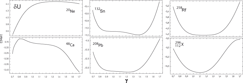
Figure 3: As a test of the plateau condition $\partial U/\partial\gamma=0$ for the Strutinsky shell correction method, the total shell correction energy $\delta U=\delta U_{P}+\delta U_{N}$ is plotted as a function of $\gamma$ for different nuclei.

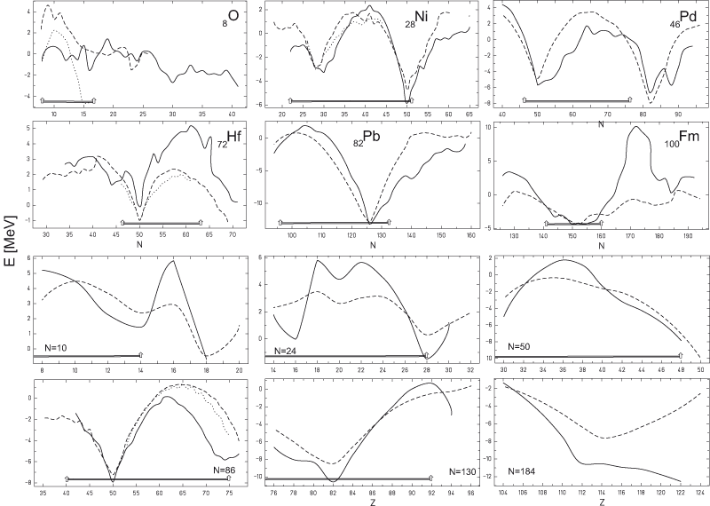
Figure 4: Comparison of calculated shell corrections $\delta U$ from the Caputo-Riemann-Riemann symmetric rotor (3) with the parameter set (49)-(56) (thick line) with the tabulated $E_{\textrm{mic}}$ from Möller [31] (dashed line). Upper two rows show values for a given $Z$ as a function of $N$, lower two rows for a given $N$ as a function of $Z$. Bars indicate the experimentally known region. The original $\epsilon_{2}$ values from [31] are used, which is the main source of error.

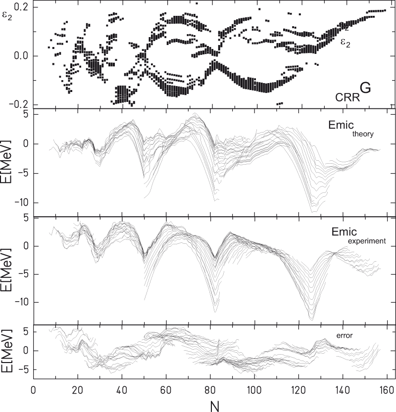
Figure 5: Comparison of calculated $E_{\textrm{mic}}$ from the Caputo-Riemann-Riemann symmetric rotor (3) with the parameter set (49)-(56), minimized with respect to $\epsilon_{2}$ with the experimental masses from Audi [38] as a function of $N$. From top to bottom the minimized $\epsilon_{2}$ values, theoretical $E_{\textrm{mic}}$, experimental microscopic contribution from the difference of experimental mass excess and and macroscopic FRLDM energy and error in $[MeV]$ are plotted.

In order to calculate the shell corrections, we introduce the following parameters:

$$\hbar\omega_{0} = 38A^{-\frac{1}{3}}[MeV]$$ (49)

$$\omega_{1} = \omega_{0}Q^{-\frac{1}{3}}$$ (50)

$$\omega_{2} = \omega_{1}$$ (51)

$$\omega_{3} = \omega_{0}Q^{\frac{2}{3}}$$ (52)

$$\alpha_{Z} = \cases{0.46+0.000220\,Z&$Z>50$\\ 0.2469+0.00448\,Z&$28<Z\leq 50$\\ 0.2793+0.00332\,Z&$Z\leq 28$\\ }$$ (53)

$$\alpha_{N} = \cases{0.41+0.000200\,N&$N>50$\\ 0.3118+0.00216\,N&$28<N\leq 50$\\ 0.2793+0.00332\,N&$N\leq 28$\\ }$$ (54)

$$\gamma = 1.1\,\hbar\omega_{0}$$ (55)

$$m = 4$$ (56)

$$a_{0} = 2.409[{\textrm{MeV}}]$$ (57)

$$a_{R} = 15.0[{\textrm{MeV}}]$$ (58)

Input parameters are the number of protons $Z$, number of neutrons $N$, the nucleon number $A=N+Z$, and the ground state quadrupole deformation $\epsilon_{2}$.

The values obtained include the frequencies (50),(51),(52), which result from a least square fit and quadratic approximation of equipotential surfaces, the fractional derivative coefficients for protons (53) and neutrons (54) which determine the level spectrum for protons and neutrons for the proton and neutron part of the shell correction energy respectively from a fit of the set of nuclids ${}^{56}_{28}\textrm{Ni}$, ${}^{100}_{50}\textrm{Sn}$, ${}^{132}_{50}\textrm{Sn}$, ${}^{208}_{82}\textrm{Pb}$ and from the requirement, that the neutron shell correction for ${}^{100}_{50}\textrm{Sn}$ should amount about $-5.1[MeV]$, (55) from the plateau condition $\partial U/\partial\gamma=0$ (see figure 3) and (56) the order of included Hermite polynomials for the Strutinski shell correction method. Finally $\hbar\omega_{0},a_{0},a_{R}$ from a fit of the experimental mass excess given in [38].

We compare our results with for the microscopic energy contribution $E_{\textrm{mic}}$ with data from Möller et. al. [31] and use their tabulated $\epsilon_{2}$ values. They have not only listed data for experimental masses but also predictions for regions, not yet confirmed by experiment.

In figure 4 we compare the calculated $\delta U$ values with the tabulated $E_{\textrm{mic}}$, which is justified for almost spherical shapes ($\epsilon_{2}\approx 0$). The results agree very well within the expected errors (which are estimated $\approx 2\,[MeV]$ for the pairing energy and $0.5\,[MeV]$ for $E_{\textrm{mic}}$), especially in the region of experimentally known nuclei.

A remarkable difference between the calculated shell correction and tabulated $E_{\textrm{mic}}$ from Möller occurs for superheavy elements ($N=184$, last picture in figure 4). While phenomenological shell models predict a pronounced minimum in the shell correction energy for $Z=114$ [33]-[37] the situation is quite different for the rotor model, where two magic shell closures at $Z=112$ and $Z=126$ are given, but the $Z=112$ shell closure is not strong enough to produce a local minimum in the shell correction energy plot as a function of $Z$. Instead, between $Z=112$ and $Z=126$, there emerges a slightly falling energy plateau, which makes the full region promising candidates for stable, long-lived superheavy elements.

While this result contradicts predictions made with phenomenological shell models, it supports recent results obtained with relativistic mean field models [7], which predict a similar behaviour in the region of super heavy elements as the proposed rotor model.

In figure 5 we have covered the complete region of available experimental data for nuclids and compare the calculated theoretical microscopic energy contribution minimized with respect to the deformation with the experimental values. The influence of shell closures is very clear. The rms-error is about $2.4[{\textrm{MeV}}]$. The maximum deviation occures between closed magic shells. Therefore in the next section we will introduce a generalization of the proposed fractional rotor model, which not only determines the magic numbers accurately but in addition determines the fine structure of the single particle spectrum correctly.

5 Fine structure of the single particle spectrum - the extended Caputo-Riemann-Riemann symmetric rotor

In the previous section we have demonstrated, that the Caputo-Riemann-Riemann symmetric rotor correctly determines the magic numbers in the single particle spectra for neutrons and protons. However, there remains a significant difference between calculated and experimental ground state masses for nuclei with nucleon numbers far from magic shell closures. This is a strong indication for the fact, that the fine structure of the single particle levels is not yet correctly reproduced.

We therefore propose the following generalization of the Caputo-Riemann-Riemann symmetric rotor group:

$${{}_{\textrm{\tiny{C3C2R3R3}}}}G\supset{{}_{\textrm{\tiny{C}}}}SO^{\alpha}(3)\supset{{}_{\textrm{\tiny{C}}}}SO^{\alpha}(2)\supset{{}_{\textrm{\tiny{R}}}}SO^{\alpha}(3)\supset{{}_{\textrm{\tiny{R}}}}SO^{\alpha}(3)$$ (59)

with the Casimir operators (2) and (2) it follows for the Hamiltonian $H$:

$$H=\frac{\omega_{1}}{\hbar}{{}_{\textrm{\tiny{C}}}}L_{1}^{2}(\alpha)+B\omega_{0}{{}_{\textrm{\tiny{C}}}}L_{z_{1}}(\alpha)+\frac{\omega_{2}}{\hbar}{{}_{\textrm{\tiny{R}}}}L_{2}^{2}(\alpha)+\frac{\omega_{3}}{\hbar}{{}_{\textrm{\tiny{R}}}}L_{3}^{2}(\alpha)$$ (60)

with the free parameters $\omega_{1},\omega_{2},\omega_{3},B$, where $B$ may be called fractional magnetic field strength in units $[\hbar\omega_{0}]$.

Imposing the same symmetries (25),(26) as in the case of the symmetric Caputo-Riemann-Riemann rotor, the eigenvalues of the Hamiltonian (60) are given as

$$E(\alpha) = \hbar\omega_{1}{{}_{\textrm{\tiny{C}}}}[2n_{1}][2n_{1}+1]+B\hbar\omega_{0}{{}_{\textrm{\tiny{C}}}}[2n_{1}]+$$ (62)

$$\hbar\omega_{2}{{}_{\textrm{\tiny{R}}}}[2n_{2}][2n_{2}+1]+\hbar\omega_{3}{{}_{\textrm{\tiny{R}}}}[2n_{3}][2n_{3}+1]$$

$$= \sum_{i=1}^{3}\hbar\omega_{i}\frac{\Gamma(1+(2n_{i}+1)\alpha)}{\Gamma(1+(2n_{i}-1)\alpha)}-\delta_{n_{1}0}\hbar\omega_{1}\frac{\Gamma(1+\alpha)}{\Gamma(1-\alpha)}$$

$$+B\hbar\omega_{0}\frac{\Gamma(1+(2n_{1})\alpha)}{\Gamma(1+(2n_{1}-1)\alpha)}-\delta_{n_{1}0}B\hbar\omega_{0}\frac{1}{\Gamma(1-\alpha)}$$

$$\qquad\qquad\qquad\qquad\qquad n_{1},n_{2},n_{3}=0,1,2,..$$

on a basis $|2n_{1}2n_{1}2n_{2}2n_{2}2n_{3}2n_{3}>$.

We call this model the extended Caputo-Riemann-Riemann symmetric rotor. The additional ${{}_{\textrm{\tiny{C}}}}L_{z_{1}}(\alpha)$ term yields a level splitting of the harmonic oscillator set of magic numbers $n_{\textrm{magic 1}}$ (34), while the multiplicity of the $n_{\textrm{magic 2}}$ set (37) remains unchanged, since this set is characterized by $n_{1}=0$. This is exactly the behaviour needed to describe the experimentally observed fine structure, as can be deduced from the right hand side of figure 2.

In order to clearly demonstrate the influence of the additional term, we first investigate the level spectrum for the spherical (31) and idealized case $\alpha=1/2$.

The level spectrum (62) simply results as:

$$E(\alpha=1/2) = \hbar\omega_{0}(n_{1}+n_{2}+n_{3}+\frac{3}{2}-\frac{1}{2}\delta_{n_{1}0})$$ (64)

$$+B\hbar\omega_{0}(\frac{n_{1}!}{\Gamma(1/2+n_{1})}-\frac{1}{\Gamma(1/2)}\delta_{n_{1}0})$$

$$= \hbar\omega_{0}(n_{1}+n_{2}+n_{3}+\frac{3}{2}-\frac{1}{2}\delta_{n_{1}0})$$

$$+\frac{B\hbar\omega_{0}}{\sqrt{\pi}}(\frac{2^{n_{1}}n_{1}!}{(2n_{1}-1)!!}-\delta_{n_{1}0})$$

where $!!$ denotes the double factorial.

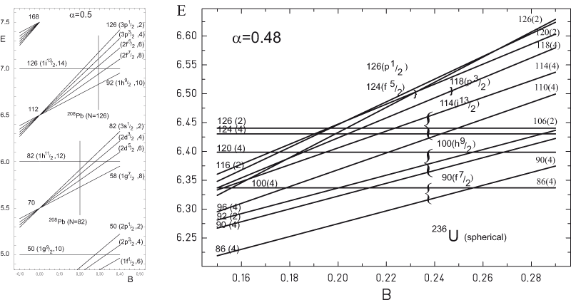
Figure 6: For $\alpha=1/2$, on the left side the level spectrum for the extended Caputo-Riemann-Riemann symmetric rotor (62) is plotted as a function of the fractional magnetic field strength $B$. The levels are labeled according to the corresponding $[Nlj_{z}]$ Nilsson scheme and the multiplicity is given. For $\alpha=0.48$ the resulting level sequence near $N\approx 126$ is plotted on the right. At $B\approx 0.25$ the resulting spectrum coincides with the corresponding spherical Nilsson level spectrum. Brackets indicate the proposed appropriate combinations of rotor levels.

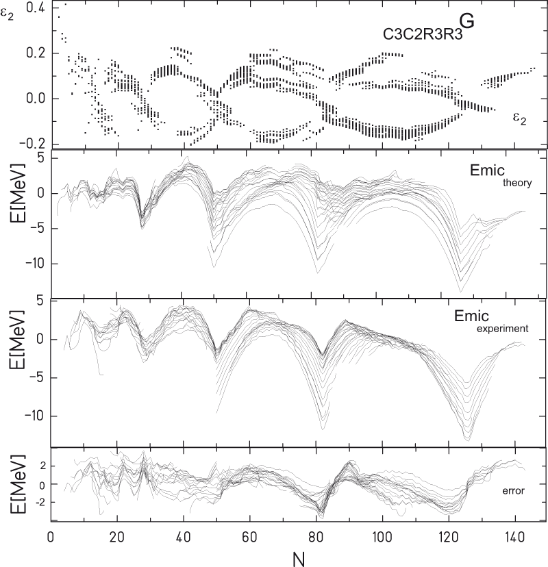
Figure 7: Comparison of calculated $E_{\textrm{mic}}$ from the extended Caputo-Riemann-Riemann symmetric rotor (62) with the parameter set (65)-(68), minimized with respect to $\epsilon_{2}$ with the experimental masses from Audi [38] as a function of $N$. From top to bottom the minimized $\epsilon_{2}$ values, theoretical and experimental masses and error in $[MeV]$ are plotted.

On the left side of figure 6 this spectrum is plotted in units $[\hbar\omega_{0}]$. Single levels are labeled according to the Nilsson-scheme and multiplicities are given in brackets. For small fractional field strength $B$ the resulting spectrum exactly follows the schematic level diagram of a phenomenological shell model with spin-orbit term, as demonstrated e.g. by Goeppert-Mayer [1].

A small deviation from the ideal $\alpha=1/2$ value reproduces the experimental spectra accurately: For $\alpha=0.48$ the resulting level spectrum is given on the right hand side of figure 6. Obviously there is an interference of two effects: First, for $\alpha\neq 1/2$ now the degenerated levels of both magic sets split up and second the fractional magnetic field $B$ acts on the subset $n_{\textrm{magic 1}}$. For $B\approx 0.25$ the spectrum may be directly compared with the spherical Nilsson level scheme, which is given for neutrons between $82\leq N\leq 126$ as $2f{\frac{7}{2}}$, $1h{\frac{9}{2}}$, $1i{\frac{13}{2}}$, $3p{\frac{3}{2}}$, $2f{\frac{5}{2}}$, $3p{\frac{1}{2}}$, see e.g. results of [39], which corresponds to a sequence of sub-shells at $90,100,114,118,124,126$. This sequence is correctly reproduced with the extended Caputo-Riemann-Riemann symmetric rotor.

With the parameter set, which is obtained by a fit with the experimental masses of Ca-, Sn- and Pb-isotopes

$$\hbar\omega_{0} = 28A^{-\frac{1}{3}}[MeV]$$ (65)

$$\alpha_{Z} = \cases{0.480+0.00022\,Z&$Z>50$\\ 0.324+0.00332\,Z&$Z\leq 50$\\ }$$ (66)

$$\alpha_{N} = \cases{0.446+0.00022\,N&$N>29$\\ 0.356+0.00332\,N&$N\leq 29$\\ }$$ (67)

$$B = 0.27$$ (68)

the experimental masses are reproduced with an rms-error of $1.7[{\textrm{MeV}}]$. Results are given in figure 7.

The deformation parameters, obtained by minimization of the total energy, are to a large extend consistent with values given in [31] e.g. for ${}^{264}{\textrm{Hs}}_{108}$ we obtain $\epsilon_{2}=0.22$, which conforms with Möller‘s ($\epsilon_{2}=0.2$) and Rutz‘s results [8]. However, there occur discrepancies mostly for exotic nuclei. For example our calculations determine the nucleus ${}^{42}{\textrm{Si}}$ to be almost spherical, while Möller predicts a definitely oblate shape.

Finally, defining a nucleus with $\epsilon_{2}>0.05$ as prolate and with $\epsilon_{2}<-0.05$ as oblate the amount of prolate shapes is about $74\%$ of all deformed nuclei. This is close to the value of $82\%$ [40], obtained with the Nilsson model using the standard parameters.

Summarizing the results presented, the proposed extended Caputo-Riemann-Riemann symmetric rotor describes the ground state properties of nuclei with reasonable accuracy. We have demonstrated, that the nuclear shell structure may indeed be successfully described on the basis of a dynamical symmetry model.

The advantages of this model, compared to phenomenological shell and relativistic mean field models respectively are obvious:

Magic numbers are predicted, they are not the result of a fit with a phenomenological $ls$-term. There are no potential-terms or parametrized Skyrme-forces involved and finally, all results may be calculated analytically.

The results obtained encourage further investigations in this field. The next steps should include the pairing energy term and parameters should be determined by a more sophisticated fit procedure. With these additional contributions the model will most probably describe nuclear properties with at least similar accuracy as the models currently used.

6 Conclusion

Based on the Riemann- and Caputo definition of the fractional derivative we used the fractional extensions of the standard rotation group $SO(3)$ to construct a higher dimensional representation of a fractional rotation group with mixed derivative types.

We obtained an extended symmetric rotor model, which predicts the sequence of magic proton and neutron numbers accurately. Furthermore we have shown, that the ground state properties of nuclei can be reproduced correctly within the framework of this model.

Hence we have demonstrated, that a dynamic symmetry, generated by mixed fractional type rotation groups is indeed realized in nature.

7 Acknowledgment

We thank A. Friedrich for useful discussions.

8 References

References

- [1] Goeppert-Mayer M Phys. Rev. 75 (1949) 1669.
- [2] Haxel F P , Jensen J H D and Suess H D Phys. Rev. 75 (1949) 1769.
- [3] Nilsson S G Kgl. Danske Videnskab. Selsk. Mat.-Fys. Medd. 29, (1955) 431.
- [4] Nilsson S G et al. Nucl. Phys. A 131, (1969) 1.
- [5] Hofmann S and Münzenberg G Reviews of Modern Physics, 72, (2000) 733.
- [6] Rufa M et al. Phys. Rev. C 38 (1988) 390.
- [7] Bender M, Nazarewicz W, Reinhard P-G Phys. Lett. B515 (2001) 42.
- [8] Rutz K et al. Phys. Rev. C 56 (1997) 238.
- [9] Kruppa A T et al. Phys. Rev. C 61 (2000) 034313.
- [10] Elsasser W M J. Phys. Radium 5 (1934) 635.
- [11] Elliott J P Proc. Roy. Soc. London A245, (1958) 128.
- [12] Iachello F and Arima A, 1987 The Interacting Boson Model Cambridge University Press, Cambridge.
- [13] Miller K and Ross B 1993 An Introduction to Fractional Calculus and Fractional Differential Equations Wiley, New York.
- [14] Oldham K B and Spanier J 2006 The Fractional Calculus, Dover Publications, Mineola, New York.
- [15] Podlubny I 1999 Fractional Differential equations, Academic Press, New York.
- [16] Herrmann R 2008 Fraktionale Infinitesimalrechnung - Eine Einführung für Physiker, BoD, Norderstedt, Germany
- [17] Leibniz G F Sep 30, 1695 Correspondence with l‘Hospital, manuscript.
- [18] Euler L Commentarii academiae scientiarum Petropolitanae 5, (1738) pp. 36-57.
- [19] Liouville J 1832 J. cole Polytech., 13, 1-162.
- [20] Riemann B Jan 14, 1847 Versuch einer allgemeinen Auffassung der Integration und Differentiation in: Weber H (Ed.), Bernhard Riemann’s gesammelte mathematische Werke und wissenschaftlicher Nachlass, Dover Publications (1953), 353.
- [21] Caputo M Geophys. J. R. Astr. Soc. 13, (1967) 529.
- [22] Weyl H Vierteljahresschrift der Naturforschenden Gesellschaft in Zürich 62, (1917) 296.
- [23] Feller W Comm. Sem. Mathem. Universite de Lund, (1952) 73-81.
- [24] Riesz M Acta Math. 81, (1949) 1.
- [25] Grünwald A K Z. angew. Math. und Physik 12, (1867) 441.
- [26] Herrmann R J. Phys. G: Nucl. Part. Phys. 34, (2007), 607.
- [27] Herrmann R arxiv:math-ph/0510099.
- [28] Maruhn J and Greiner W Z. Physik 251, (1972) 431.
- [29] Strutinsky V M Nucl. Phys. A95, (1967) 420.
- [30] Strutinsky V M Nucl. Phys. A122, (1968) 1.
- [31] Möller et. al. Atomic Data Nucl. Data Tables 59, (1995) 185.
- [32] Herrmann R arxiv:gen-ph/0801.0298.
- [33] Myers W D and Swiatecki W J Nucl. Phys. 81, (1966) 1.
- [34] Sobiczewski A, Gareev F A and Kalinkin B N Phys. Lett. 22 (1966), 500.
- [35] Meldner H Ark. Fys. 36, (1967) 593.
- [36] Mosel U, Fink B and Greiner W Contribution to ”Memorandum Hessischer Kernphysiker” Darmstadt, Frankfurt, Marburg, (1966).
- [37] Mosel U and Greiner Z. f. Physik 217 (1968) 256, 222 (1968) 261.
- [38] Audi G, Wapstra A H and Thibault C Nucl. Phys. A729 (2003) 337.
- [39] Scharnweber D, Mosel U and Greiner W Phys. Rev. Lett. 24 (1970) 601.
- [40] Tajima N and Suzuki N Phys. Rev. C 64 (2001) 037301.