Thermal destruction of chiral order in a two-dimensional model of coupled trihedra

Abstract

We introduce a minimal model describing the physics of classical two-dimensional (2D) frustrated Heisenberg systems, where spins order in a non-planar way at $T=0$. This model, consisting of coupled trihedra (or Ising-$\mathbb{R}P^{3}$ model), encompasses Ising (chiral) degrees of freedom, spin-wave excitations and $\mathbb{Z}_{2}$ vortices. Extensive Monte Carlo simulations show that the $T=0$ chiral order disappears at finite temperature in a continuous phase transition in the $2D$ Ising universality class, despite misleading intermediate-size effects observed at the transition. The analysis of configurations reveals that short-range spin fluctuations and $\mathbb{Z}_{2}$ vortices proliferate near the chiral domain walls explaining the strong renormalization of the transition temperature. Chiral domain walls can themselves carry an unlocalized $\mathbb{Z}_{2}$ topological charge, and vortices are then preferentially paired with charged walls. Further, we conjecture that the anomalous size-effects suggest the proximity of the present model to a tricritical point. A body of results is presented, that all support this claim: (i) First-order transitions obtained by Monte Carlo simulations on several related models (ii) Approximate mapping between the Ising-$\mathbb{R}P^{3}$ model and a dilute Ising model (exhibiting a tricritical point) and, finally, (iii) Mean-field results obtained for Ising-multispin Hamiltonians, derived from the high-temperature expansion for the vector spins of the Ising-$\mathbb{R}P^{3}$ model.

I Introduction

On bipartite lattices, the energy of the classical Heisenberg, as well as XY, antiferromagnet is minimized by collinear spin configurations. Any two such ground states can be continuously transformed into one another by a global spin rotation. By contrast, it is quite common that the ground state manifold of frustrated magnets comprises several connected components, with respect to global spin rotations, that transform into one another under discrete symmetry only. Examples include Villain’s fully frustrated XY model, villain77 the $J_{1}-J_{2}$ Heisenberg model on the square lattice, ccl90 ; weber03 the $J-K_{4}$ model on the triangular lattice, momoi97 the $J_{1}-J_{3}$ model on the square lattice, cs04 and the $J_{1}-J_{2}$ model on the kagomé lattice. domenge05 ; domenge08

The Mermin-Wagner theorem mermin66 forbids the spontaneous breakdown of continuous symmetries, such as spin rotations, at any $T>0$ in two dimensions (2D). However, as was first noticed by Villain, villain77 the breakdown of the discrete symmetries relating the different connected components of the ground state manifold may indeed give rise to finite temperature phase transition(s). Such transitions have been evidenced numerically in a number of frustrated systems, with either XY numerics_FFXY or Heisenberg spins. momoi97 ; weber03 ; domenge05 ; domenge08

We are interested in a particular class of models with Heisenberg spins, where the ground state has non-planar long-range order. momoi97 ; domenge05 ; domenge08 In this case the ground state is labeled by an $O(3)$ matrix. Hence the ground state manifold is $O(3)=SO(3)\times\mathbb{Z}_{2}$ which breaks down into two copies of $SO(3)$. The two connected components, say 1 and 2, are exchanged by a global spin inversion ($\vec{S}_{i}\to-\vec{S}_{i}$) and may be labeled by opposite scalar chiralities $\vec{S}_{i}\cdot(\vec{S}_{j}\times\vec{S}_{k})$. Hence we introduce a local Ising variable $\sigma(\vec{r})=\pm 1$ which measures whether the spins around $\vec{r}$ have the chirality of sector 1 or 2. At $T=0$ the chiralities $\sigma(\vec{r})$ are long-range ordered and the ground state belongs to a given sector. On the other hand, at high enough temperature the system is fully disordered. Hence, on very general grounds we expect the spontaneous breakdown of the spin inversion symmetry, associated to $\langle\sigma(\vec{r})\rangle\neq 0$, at some intermediate temperature.

Further, from the standpoint of Landau-Ginzburg theory, one anticipates a critical transition in the 2D Ising universality class. However, of the two relevant models studied so far, momoi97 ; domenge05 ; domenge08 none shows the signature of an Ising transition. Instead, as was pointed out by some of us in Ref. domenge08, , the existence of underlying (continuous) spin degrees of freedom complicates the naive Ising scenario, and actually drives the chiral transition towards first-order.

To get a better sense of this interplay between discrete and continuous degrees of freedom, it is useful to remember that in 2D, although spin-waves disorder the spins at any $T>0$, the spin-spin correlation length may be huge ($\xi\sim\exp(-A/T)$) at low temperature, bz76 especially in frustrated systems. Hence, it is likely that the effective, spin-wave mediated, interaction between the emergent Ising degrees of freedom extends significantly beyond one lattice spacing, even at finite temperature and in 2D.

Further, we point out that the excitations built on the continuous degrees of freedom are not necessarily limited to spin-waves. To be more specific, if the connected components of the ground state manifold are not simply connected, as is the case for $SO(3)$, then there also exists defects in the spin textures. Here, $\Pi_{1}(SO(3))=\mathbb{Z}_{2}$ implies that $\mathbb{Z}_{2}$ point defects (vortices in 2D) are topologically stable. Clearly these additional excitations may also affect the nature of the transition associated to the Ising degrees of freedom. In fact, it was shown on one example domenge08 that the first-order chiral transition is triggered by the proliferation of these defects.

In this paper we aim at clarifying the nature of the interplay between the different types of excitations found in Heisenberg systems with non-planar long-range order at $T=0$. Note that the associated unit cell is typically quite large, which severely limits the sample sizes amenable to simulations. Hence, we introduce a minimal model with the same physical content as the frustrated models studied in Refs momoi97, ; domenge05, ; domenge08, .

As was already mentioned, in the above frustrated spin systems, the spin configuration at $T=0$ is entirely described by an $O(3)$ matrix, or equivalently a trihedron in spin space. At low temperature, the spin long-range order is wiped out by long wavelength spin waves, but from the considerations above we anticipate that, at low enough temperatures, the description in terms of trihedra in spin space still makes sense, at least locally. To be more specific, we assign three unit vectors $\vec{S_{i}}^{a}$ ($a=1,2,3$) to every site $i$ of the square lattice, subject the orthogonality constraint

$$\vec{S_{i}}^{a}\cdot\vec{S_{i}}^{b}=\delta^{a,b},$$ (1)

and we assume the following interaction energy

$$E=-\sum_{a=1}^{3}\sum_{\langle i,j\rangle}\vec{S_{i}}^{a}\cdot\vec{S_{j}}^{a}.$$ (2)

Hence we consider three ferromagnetic Heisenberg models, tightly coupled through the rigid constraint (1). At $T=0$, the energy is minimized by any configuration with all trihedra aligned, and the manifold of ground states is $O(3)$, as desired. This alone ensures the existence of the three types of excitations: i) $SO(3)$ spin waves (corresponding to the rotation of the trihedra), ii) $SO(3)$ vortices, and iii) Ising (chiral) degrees of freedom, corresponding to the right or left-handedness of the trihedra.

The present study is devoted to the model defined by Eqs. 1 and 2.

In Section II we reformulate this model more conveniently in terms of chiralities and four-dimensional (4D) vectors, yielding the so-called Ising-$\mathbb{R}P^{3}$ model. For clarity we first consider a simplified version of this model where the chirality variables are frozen, and we use this setup to detail our method to detect vortex cores and analyze their spatial distribution.

In section III, we return to the full Ising-$\mathbb{R}P^{3}$ model and evidence the order-disorder transition of the Ising variables at finite-temperature. The nature of the transition is asserted by a thorough finite-size analysis using Monte-Carlo simulations. To clarify the nature of the interplay between discrete and continuous degrees of freedom we perform a microscopic analysis of typical configurations.

For the most part, the remainder of our work originates from the observation of peculiar intermediate size effects at the transition. This leads us to argue that the present model lies close to a tricritical point in some parameter space.

To support our claim we first introduce and perform Monte Carlo simulations on two modified versions of our model that i) preserve the $O(3)$ manifold of ground states, and ii) lead to a first-order transition of the Ising variables.

This is further elaborated on in section IV, where we draw an analogy between the Ising-$\mathbb{R}P^{3}$ model and the large $q$ Potts model. Another analogy, this time to a dilute Ising model, is drawn in section V, where we argue that the regions of strong misalignment of the trihedra, near Ising domain walls, can be treated as “depletions” in the texture formed by the 4D-vectors.

Finally, in Section VI we take another route and trace out the continuous degrees of freedom perturbatively, resulting in an effective model for the Ising variables, that we proceed to study at the mean-field level.

II Basics of the model

II.1 Ising-$\mathbb{R}P^{3}$ formulation

The model defined by Eqs. 1 and 2 can be conveniently reformulated as an Ising model coupled to a four-component spin system with biquadratic interactions. Indeed, every trihedron is represented by an $SO(3)$ matrix $M_{i}$ and a chirality $\sigma_{i}=\pm 1$:

$$\vec{S_{i}}^{1}=\sigma_{i}M_{i}\left[\begin{array}[]{c}1\\ 0\\ 0\end{array}\right],\,\vec{S_{i}}^{2}=\sigma_{i}M_{i}\left[\begin{array}[]{c}0\\ 1\\ 0\end{array}\right],\,\vec{S_{i}}^{3}=\sigma_{i}M_{i}\left[\begin{array}[]{c}0\\ 0\\ 1\end{array}\right].$$ (3)

Using these variables, Eq. 2 reads

$$E=-\sum_{\langle i,j\rangle}\sigma_{i}\sigma_{j}{\rm Tr}\left[(M_{i})^{t}M_{j}\right]$$ (4)

The isomorphism between $SO(3)$ and $SU(2)/\left\{1,-1\right\}$, maps a rotation $M(\theta,\vec{n})$ of angle $\theta$ about the $\vec{n}$ axis onto the pair of $SU(2)$ matrices $\pm\exp(i\frac{\theta}{2}\vec{n}\cdot\vec{\sigma})$, where the components of $\vec{\sigma}$ are the Pauli matrices. The latter can be written using two opposite 4D real vectors $\pm\vec{v}=\pm(v_{0},v_{x},v_{y},v_{z})$ with $\vec{v}^{2}=1$:

$$\exp\left(i\frac{\theta}{2}\vec{n}\cdot\vec{\sigma}\right)=\left[\begin{array}[]{cc}v_{0}+iv_{z}&iv_{x}+v_{y}\\ iv_{x}-v_{y}&v_{0}-iv_{z}\end{array}\right]$$ (7)

$$v_{0}=\cos(\theta/2)\,\,,\,\,v_{a}=n_{a}\sin(\theta/2).$$ (8)

Irrespective of the local (arbitrary) choice of representation $\pm\vec{v}_{i}$, one has

$${\rm Tr}\left[(M_{i})^{t}M_{j}\right]=4(\vec{v}_{i}\cdot\vec{v}_{j})^{2}-1$$ (9)

whence the energy reads

$$E=-\sum_{\langle i,j\rangle}\sigma_{i}\sigma_{j}\left(4(\vec{v}_{i}\cdot\vec{v}_{j})^{2}-1\right).$$ (10)

II.2 $\mathbb{Z}_{2}$ vortices in the fixed-chirality limit

Here we first consider the simplified case where the Ising degrees of freedom are frozen to, say, $\sigma_{i}=+1$. In this limit we recover the so-called $\mathbb{R}P^{3}$ model,  which contains both spin-waves and $\mathbb{Z}_{2}$ vortices, and describes interacting $SO(3)$ matrices. Together with related frustrated spin models (Heisenberg model on the triangular lattice for instance), the $\mathbb{R}P^{3}$ model has been the central subject of a number of studies focusing on a putative binding-unbinding transition of the $\mathbb{Z}_{2}$ vortices at finite temperature. km84 ; ks87 ; dr89 ; adj90 ; kz92 ; adjm92 ; sy93 ; sx95 ; caracciolo93 ; hasenbusch96 ; wae00 ; cadm01 This is a delicate and controversial issue, which is not essential to the present work. Instead, we merely discuss some properties of the vortex configurations that will be useful for comparison with the full $O(3)$ (or Ising-$\mathbb{R}P^{3}$) model.

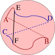
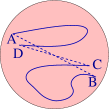
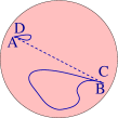
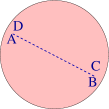
Figure 1: (Color online). $SO(3)$ can be represented by a ball of radius $\pi$. A rotation of angle $\theta\in[0,\pi]$ around the $\vec{n}$ axis is represented in this ball by the extremity of the vector $\theta\vec{n}$. Two opposite points of the surface (joined by a dashed line) represent the same rotation. A loop with an odd number of crossings, such as $ABFEA$ or $CDEFC$, cannot be continuously shrunk to a point. This is not the case when the number of crossings is even: a) $ABCDEA$ crosses the surface both at (AB) and (CD). b)-c) It can be continuously deformed to collapse points $B$ on $C$, and $A$ on $D$. d) $AD$ and $BC$ become contractible closed loops, that collapse on identical points.

To locate the topological point defects (vortex cores) we resort to the usual procedure: Consider a closed path, $\mathcal{L}$, on the lattice, running through sites ${i_{0}},\cdots,{i_{n-1}},{i_{n}\equiv i_{0}}$. $\mathcal{L}$ induces a loop $\mathcal{C_{L}}$ in the order parameter space, defined by the matrices $M_{i_{0}},\cdots,M_{i_{n-1}},M_{i_{n}}$ (in this space the path between $M_{i_{k}}$ and $M_{i_{k+1}}$ is defined as the “shortest one”). The homotopy class of $\mathcal{C_{L}}$ is an element of $\Pi_{1}$. If it is the identity, then the $\mathcal{C_{L}}$ loop is contractible. Otherwise, $\mathcal{L}$ surrounds (at least) one topological defect. mermin

In the $\mathbb{R}P^{3}$ model, the fundamental group is $\Pi_{1}(SO(3))=\mathbb{Z}_{2}$, so that the topological charge can take only two values: the homotopy class of $\mathcal{C_{L}}$ correspond to the parity of the number of point defects enclosed in $\mathcal{L}$. This is to be contrasted with the better-known $SO(2)$ vortices, associated, for instance, to the $XY$ model: the latter carry an integer charge ($\Pi_{1}(SO(2))=\mathbb{Z}$) while the former carry merely a sign.

The number of $\mathbb{Z}_{2}$ vortices of a given configuration is obtained by looking for vortex cores on each elementary plaquette of the lattice. The vorticity $\Omega(p)$ of a square plaquette $p$ is computed using by mapping $SO(3)$ to $\mathbb{R}P^{3}=S^{3}/\mathbb{Z}_{2}$: on every site $i$ we arbitrarily choose one of the two equivalent representations $\pm\vec{v}_{i}$ of the local $SO(3)$ matrix and compute

$$\Omega(p)=\prod_{\square_{p}}\text{sign}(\vec{v}_{i}.\vec{v}_{j}),$$ (11)

where $i$ and $j$ are nearest neighbors and the product runs over the four edges of ${\square_{p}}$. The associated closed loop in $SO(3)$ is non-contractible when the plaquette hosts a vortex core, and is identified by $\Omega(p)=-1$. Note that $\Omega(p)$ is a “gauge invariant” quantity, i.e. it is independent of the local choice of representation $\pm\vec{v}_{i}$, as it should be.

We performed a Monte Carlo simulation of the $\mathbb{R}P^{3}$ model using a Wang-Landau algorithm, detailed in Appendix A. In the upper panel of Fig. 2 we plot the vortex density $n_{\Omega}$, defined as the number of plaquettes hosting a vortex core divided by the total number of plaquettes.

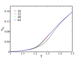
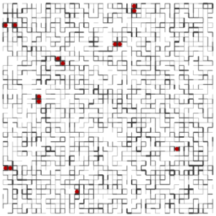
Figure 2: (Color online) Uniform frozen chirality model (see text paragraph II.2). Top: Vortex density $n_{\Omega}$ versus temperature $T$, from $L=16$ to $L=64$, from bottom to top. Bottom: Thermalized configuration at $T\simeq 1.1$ on a system of size $L=72$ (only a 45$\times$45 square snippet is shown). Square plaquettes carrying a $\mathbb{Z}_{2}$ vortex core are denoted by a (red) bullet. The width of each bond $(i,j)$ is proportional to $B_{ij}=1-(\vec{v}_{i}\cdot\vec{v}_{j})^{2}$ (by slices of $1/8$). Bonds with $B_{ij}\leq 1/8$ are not drawn.

Vortices are seen to appear and the density increases upon increasing the temperature from $T\simeq 1$. However, no critical behavior (scaling) is observed upon increasing the system size. The latter is also true of other simple thermodynamic quantities, such as the energy or the specific heat, although the latter is maximum when the increase in $n_{\Omega}$ is steepest, at $T\simeq 1.3$. 

A typical configuration is shown in the lower panel of Fig. 2, at a temperature $T=1.1$, about $20\%$ lower than that of the maximum of the specific heat. Plaquettes hosting a vortex core are indicated by a (red) bullet. Note that $n_{\Omega}$ is rather small at this temperature, and that all vortices are paired, except for two, evidencing the strong binding of the vortices.

In the same figure the width of every bond $(i,j)$ is proportional to $B_{ij}=1-(\vec{v}_{i}\cdot\vec{v}_{j})^{2}$ and indicates the relative orientation of the two 4D-vectors $\vec{v}_{i}$ and $\vec{v}_{j}$. $B_{ij}=0$ (no segment) corresponds to parallel 4D-vectors (or identical trihedra), which minimizes the bond energy ( $E_{ij}=-3$). In particular, all bonds have $B_{ij}=0$ at $T=0$. On the contrary, $B_{ij}=1$ (thick black segment) indicates a maximally frustrated bond ($E_{ij}=+1$) with orthogonal 4D-vectors (the two trihedra differ by a rotation of angle $\pi$). Figure 2 shows that the vortex cores are located in regions of enhanced short-range fluctuations of the continuous variables (represented by thick bonds), but that the converse is not necessarily true.

III Numerical simulations of the Ising–$\mathbb{R}P^{3}$ model

We now return to the full Ising-$\mathbb{R}P^{3}$ model, defined in Eq. 10. We report results of Monte Carlo simulations, using the Wang-Landau algorithm described in Appendix A, for linear sizes up to $L=88$ with periodic boundary conditions.

III.1 Specific heat and energy distribution

Once the Ising degrees of freedom are relaxed, the maximum of the specific heat diverges with the system size, indicating a phase transition. Further, the scaling as $\sim\log(L)$ (Fig. 3) for the largest $L$ suggests a continuous transition in the Ising-2D universality class.

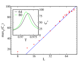
Figure 3: (Color online) Maximum value of the specific heat as a function of system size $L$. The scaling at large $L$ is correctly reproduced by the affine log fit $A+B\ln(L)$ (straight line). Inset: specific heat $C_{v}$ versus temperature $T$ for $L=64$ and $80$ from right to left.

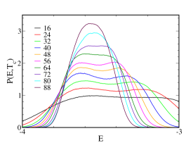
Figure 4: (Color online) Probability distribution $P(E,T_{c})$ of the energy per site at $T_{c}(L)$ for increasing linear $L$, from $L=16$ to $L=88$, from bottom to top. $T_{c}(L)$ is the temperature where $C_{v}$ is maximum. A double-peak is visible for $L\lesssim 60$, and disappears for $L=72$ and $L=80$.

To ascertain the continuous nature of the transition, we computed the probability distribution $P(E,T=T_{c})$ of the energy per site, obtained from the density of states $g(E)$ (Fig. 4). Here $T_{c}(L)$ is defined as the temperature where the specific heat is maximum. Rather surprisingly, from small to intermediate lattice sizes, $P(E,T=T_{c})$ shows the bimodal structure characteristic of a first-order transition. However, this feature disappears smoothly upon increasing the system size, and a single peak finally emerges for $L\geq 72$.

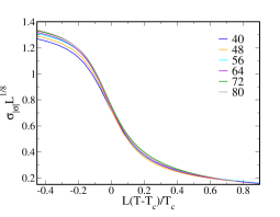
(a)

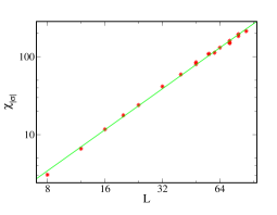
(b)

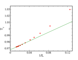
(c)

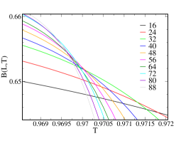
(d)

Figure 5: (Color online) Finite-size scaling at, or near, the transition temperature. a) Rescaled chirality (Eq. 12) versus rescaled temperature for $40\leq L\leq 80$. b) Log-log plot of the maximum of the Ising susceptibility vs. $L$. c) Scaling of the maximum of the specific heat vs. $1/L$ (log-linear plot). d) Evolution of the Binder cumulant $B(L,T)$ with temperature, from $L=16$ to $L=88$, from bottom to top.

Hence we claim that the phase transition is continuous indeed, in the Ising-2D universality class, although the scaling and energy distribution at moderate sizes is misleading. This peculiar finite-size behavior evidences a large but finite length scale whose exact nature has not been elucidated so far. We conjecture that it may be related to the proximity, in some parameter space, to a tricritical point where the transition becomes discontinuous. Further arguments in support to this claim will be provided in Sections III.5, IV and V.

III.2 Ising order parameter

The ordering of the chirality variables $\sigma_{i}$ is probed by the following Ising order parameter:

$$\sigma=\left<\frac{1}{N}\left|\sum_{i}\sigma_{i}\right|\right>,$$ (12)

where $N$ is the number of sites. With the results above in mind we analyze the finite-size effects on the chirality using the scaling law $L^{\beta/\nu}\sigma=f\left(L^{1/\nu}\left(\frac{T-T_{c}}{T_{c}}\right)\right)$ with $\beta=1/8$ and $\nu=1$. Fig. 5(a) shows a data collapse of the Ising order parameter for $40\leq L\leq 88$, in agreement with the 2D-Ising critical scenario ($\beta=1/8$ and $\nu=1$). Figure 5(b) shows the scaling of the maximum of the Ising susceptibility $\chi_{\sigma}$ versus $L$. The slope $\gamma/\nu=1.76\pm 0.02$ is very close to the expected value of 7/4. We also plot the temperature $T_{c}(L)$ of the the maximum of the specific heat at size $L$ (Fig. 5(c)), showing the expected asymptotic scaling $T_{c}(L)\sim T_{\infty}+A/L^{1/\nu}$ with $\nu=1$. Finally, we computed the fourth-order Binder cumulant

$$B(L,T)=1-\frac{1}{3}\frac{\langle\sigma^{4}\rangle}{\langle\sigma^{2}\rangle^{2}}$$ (13)

which shows a characteristic $L$-independent crossing at $T_{c}\simeq 0.97$ (Fig. 5(d)). Note however that the value of the cumulant at the crossing $B(L=72,T_{\textrm{crossing}})\simeq 0.65$ remains larger than the universal value of the 2D Ising model (0.6107). This discrepancy possibly originates from the fact that $L$ is not significantly larger than the crossover length-scale beyond which the two peaks in $P(E,T_{c})$ merge (Sec. III.1), making it uneasy to obtain a reliable estimate of the fourth moment of the distribution of chiralities. We also point out that similar discrepancies were observed in the simulation of other emergent Ising systems with continuous degrees of freedom. weber03 ; numerics_FFXY

III.3 $\mathbb{Z}_{2}$ vortices in the Ising-$\mathbb{R}P^{3}$ model

We now turn to the identification of $\mathbb{Z}_{2}$ vortices in the model defined in Eq. 10. The better-known case of an $SO(3)$ ground state manifold (ferromagnetically frozen chiralities) was detailed in Section. II.2 Once the chiral degrees of freedom are relaxed, the ground state manifold is enlarged to $O(3)=\mathbb{Z}_{2}\times SO(3)$ and the definition of vorticity enclosed in lattice loops requires some caution. Let us consider two sites $i$ and $j$ and their associated elements of $O(3)$, $M_{i}$ and $M_{j}$. As long as $M_{i}$ and $M_{j}$ have the same chirality, no extra difficulty arises. However, if they have opposite chiralities (determinants), then the mere existence of a continuous path connecting the two elements in $SO(3)$ is ill-posed, since they each belong to a different $SO(3)$ sector of $O(3)$. Hence the computation of the circulation $\Omega(\mathcal{L})$ makes sense only for loops $\mathcal{L}$ enclosed in a domain of uniform chirality. In particular, the computation of the $\mathbb{Z}_{2}$ vorticity on plaquettes located in the bulk of uniform domains follows the lines detailed in Section II.2 without modification.

The case of non-uniform plaquettes, sitting on a chiral domain wall, may be addressed in an indirect way. We consider a closed loop $\mathcal{L}$ that i) only visits sites with chirality $\sigma_{i}=+1$, ii) encloses a domain of opposite chirality $\sigma_{i}=-1$. i) ensures that $\Omega(\mathcal{L})$ is well defined. On the other hand one can always define unambiguously $N_{v}(\mathcal{L})$, the number of vortex cores on uniform plaquettes inside $\mathcal{L}$. If the chirality were uniform inside $\mathcal{L}$ then $\Omega(\mathcal{L})=(-1)^{N_{v}(\mathcal{L})}$ would hold. However, when $\mathcal{L}$ encloses a domain with reversed chirality, an extra contribution arises on the right hand side, coming from the non-uniform plaquettes sitting on the domain wall, which are not accounted for by $(-1)^{N_{v}(\mathcal{L})}$. Since $\Omega(\mathcal{L})=\pm 1$ we obtain $\Omega(\mathcal{L})=\epsilon_{\text{w}}(-1)^{N_{v}(\mathcal{L})}$ where $\epsilon_{\text{w}}=\pm 1$ acts as the topological charge of the chiral domain wall. As a result, the present workaround yields the total $\mathbb{Z}_{2}$ charge carried by the chiral domain wall, which is always well defined.

Figure 7(a) shows a typical configuration near $T_{c}$. Again, vortices in the bulk of Ising domains are indicated by (red) bullets A thorough study of typical configurations reveals that most of these vortex cores are actually “paired” with a nearby charged domain wall (not represented in Fig. 7(a)). Once the charge of the walls is appropriately accounted for, the total measured charge is 1 indeed. Note that such vortex/charged-wall pairs feature two $\mathbb{Z}_{2}$ charges, but involve the creation of only one vortex core. Hence they are energetically favored compared to genuine pairs of $\mathbb{Z}_{2}$ vortices in the bulk of chiral domains. This is evidenced, for instance, by the proliferation of vortices at lower temperatures in the full Ising-$\mathbb{R}P^{3}$ than in the $\mathbb{R}P^{3}$ model (compare the upper panel of Fig.2 with Fig.6(b)).

To quantify the pairing effect of $\mathbb{Z}_{2}$ vortices with charged walls, we impose a domain wall by splitting in the system in two parts with frozen but opposite chiralities (periodic boundary conditions are used). Figure 6(a) shows the excess density of vortices near the domain wall, compared to the density in the bulk of the domains, as a function of the distance to the interface for $T=1.3$. In agreement with the trend observed in Fig. 7(a), vortex/charged-wall pairs are clearly favored compared to vortex/vortex pairs in the bulk. Moreover, this effect is robust: the excess density of vortices is sizable in a wide range of temperatures. Overall we anticipate that the same mechanism will prevail near more complex interfaces, such as those obtained in the full Ising-$\mathbb{R}P^{3}$ model at equilibrium.

For completeness, we computed the core vortex density $n_{\Omega}$ (defined as the number of vortex cores on uniform plaquettes divided by the number of such plaquettes) as a function of temperature for different lattice sizes: the increase in the vortex density at the transition temperature (Fig. 6(b)) scales with the system size. This is apparent on the associated susceptibility $dn_{\Omega}/dT$ whose maximum scales with $L$ like the maximum of the specific heat (Fig. 6(c)). This is to be compared with the non-critical behavior of the vortex density in the $\mathbb{R}P^{3}$ model discussed in Section II.2 where $dn_{\Omega}/dT$ remains finite at all temperatures.

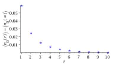
(a)

(b)

(c)

Figure 6: (Color online) a) Excess density of vortices vs. distance to the domain wall at $T=1.3$ (see text). b) Vortex density in the bulk of chiral domains vs. temperature $T$, from $L=16$ to $L=88$, from bottom to top. c) Maximum of $\left(\frac{dn_{\Omega}}{dT}\right)$ versus specific heat maximum ${\rm max_{T}(C_{v})}$ for $16\leq L\leq 88$.

III.4 Spatial correlations of discrete and continuous fluctuations

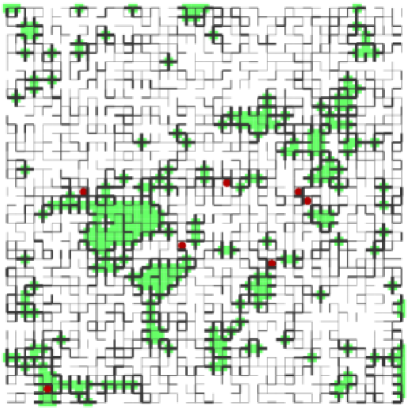
(a)

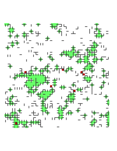
(b)

Figure 7: (Color online) Thermalized configuration at $T\simeq T_{c}$ of a system of size $L=72$ (only a $45\times 45$ square snippet is shown). Red bullets indicate elementary square plaquettes that i) host a $\mathbb{Z}_{2}$ vortex core and ii) have all four $\sigma_{i}$ equal. Plaquettes with homogeneous up (resp. down) chiralities are represented by green (resp white) squares. a) the width of bonds $(i,j)$ is proportional to $B_{ij}$ (see text). b) Bonds are drawn only if $B_{ij}>1/2$.

Figure 7(a) also reveals that the bonds standing across chiral domain walls ($\sigma_{i}\sigma_{j}=-1$) are also the most “disordered”, or thickest, ones. This strong correlation is all the more apparent in Figure 7(b), where only the highest-energy, most disordered, bonds, are represented, defined as $B_{ij}>1/2$: they are rather scarce in the bulk of Ising domains. Hence the two kinds of fluctuations (associated to the discrete Ising variables and to the continuous 4D-vectors, respectively) are both localized close to Ising domain walls. As a result, the energy barrier for the formation of a domain wall is considerably lowered compared to the pure Ising model (with all 4D-vectors frozen in a ferromagnetic configuration). This is evidenced by the low transition temperature $T_{c}=0.97$ for the Ising transition observed in the present Ising-$\mathbb{R}P^{3}$ model, compared to $T_{c}=2.269$ for the Ising model in 2D.

III.5 Small modifications of the Ising-$\mathbb{R}P^{3}$ model and tuning of the nature of the phase transition

In view of the peculiar finite-size, first-order-like, behavior of the energy distribution shown in Figure 4, we argue that the Ising-$\mathbb{R}P^{3}$ model could be near a tricritical point in some parameter space. This is consistent with the nature of the phase transitions observed in a number of related classical frustrated spin models with similar “content”, i.e. spin-waves, $\mathbb{Z}_{2}$-vortices and Ising-like chiralities. domenge05 ; domenge08 ; momoi99

In support of our claim, we present two distortions of the original Hamiltonian (10) which preserve the ground state symmetry, hence the nature of the excitations above, and show that they undergo a first-order phase transition.

As it turns out, a simple change in the bond energy

$$E_{ij}=-\sigma_{i}\sigma_{j}(4(\vec{v}_{i}\cdot\vec{v}_{j})^{2}-a)$$ (14)

from $a=1$ in the original Hamiltonian (10) to $a=1.75$, is sufficient to drive the order-disorder transition of the Ising variables towards first order. This can be seen in Figure 8, where both the maximum of the specific heat (Fig. 8(a)) and that of the chiral susceptibility (Fig. 8(b)) scale as $\sim L^{2}$. Furthermore, contrary to the Ising-$\mathbb{R}P^{3}$ case, the energy probability distribution $P(E,T=T_{c})$ remains bimodal for all lattice sizes, with a minimum that gets more and more pronounced upon increasing the system size (not shown).

Increasing $a$ from $a=1$ in (14) clearly decreases the energy gap for a chirality flip $\sigma_{i}\to-\sigma_{i}$. However, the associated modification of the entropy balance between the ordered and disordered phase is less obvious.

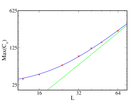
(a)

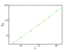
(b)

Figure 8: (Color online) a) Scaling as $L^{2}$ of the maximum of the specific heat and b) of the chiral susceptibility with increasing system size $L$ for $a=1.75$ in Eq. 14.

Entropic effects are more explicit and better controlled in the following family of continuous spin models on 2D lattices:

$$E_{ij}=-\sum_{<i,j>}\left(\frac{1+\vec{S}_{i}\cdot\vec{S}_{j}}{2}\right)^{p}.$$ (15)

Indeed, it was shown that for large enough $p$ ($p\gtrsim 100$ for $XY$ spins dsrs84 and $p\geq 16$ for Heisenberg spins bgh02 ; es02 ) these systems undergo a phase transition of the liquid-gas type. Obviously, tuning $p$ does not change the energy scale ($E_{ij}\in[0,1]$), but increasing $p$ gradually pushes the entropy toward the highest energies.

Hence we tweak the Ising-$\mathbb{R}P^{3}$ model in a similar way, with:

$$E_{ij}=-\sigma_{i}\sigma_{j}(4(\vec{v}_{i}\cdot\vec{v}_{j})^{2p}-1).$$ (16)

Once again, Monte Carlo simulations of the distorted model (16) shows the signatures of a first-order transition, for $p$ as small as $p=2$ (Fig. 9).

Overall the previous two models illustrate our claim on the proximity of the Ising transition in the Ising-$\mathbb{R}P^{3}$ model with a first-order transition.

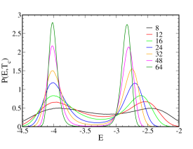
Figure 9: (Color online) Energy distributions at the transition for model (16).

IV Entropy of $\sigma_{i}\sigma_{j}$ bonds – Potts model analogy

Figure 10: (Color online) Density of state $g^{\epsilon}(E)$ for a single bond in model (10). The two colors correspond to $\epsilon=\sigma_{i}\sigma_{j}=1$ (green) and $\epsilon=-1$ (red). The lowest energy ($E=-3$ per bond) is attained when $(\vec{v}_{i}\cdot\vec{v}_{j})^{2}=1$ and $\sigma_{i}\sigma_{j}=1$.

Here we take another route and propose a simple qualitative analogy to explain how the coupling of chiralities $\sigma_{i}$ to the continuous degrees of freedom $\vec{v}_{i}$ drives the Ising transition in the Ising-$\mathbb{R}P^{3}$ model close to a first-order transition.

To that end we compute the density of states $g(E)$ for a single bond $(i,j)$. It has two contributions $g(E)=g^{+}(E)+g^{-}(E)$ depending on the value of $\epsilon=\sigma_{i}\sigma_{j}$:

$$g^{\epsilon}(E) \sim \int_{S^{3}}d^{3}\vec{v}_{i}\int_{S^{3}}d^{3}\vec{v}_{j}\delta\left(E+\epsilon(4(\vec{v}_{i}\cdot\vec{v}_{j})^{2}-1)\right)$$ (17)

$$\sim \int_{S^{3}}d^{3}\vec{v}_{i}\delta\left(E+\epsilon(4(v_{i}^{0})^{2}-1)\right)$$

where rotational invariance was used to fix $\vec{v}_{j}=[1,0,0,0]$. Explicit evaluation of the integral gives

$$g^{\epsilon}(-3\leq\epsilon E<1)=\frac{1}{2\pi}\sqrt{\frac{3+\epsilon E}{1-\epsilon E}}.$$ (18)

Figure 10 shows the evolution of $g^{\pm}(E)$ with $E$. Interestingly, the density of state is remarkably small in the vicinity of the (ferromagnetic) ground state value ($\sigma_{i}\sigma_{j}=1$, $\vec{v}_{i}\cdot\vec{v}_{j}=1$, and $E=-3$). However, if the two trihedra have opposite chiralities, the lowest energy state is attained for orthogonal vectors $\vec{v}_{i}\cdot\vec{v}_{j}=0$, with energy $E=-1$, and the associated density of states diverges.

This strong entropy unbalance between ordered ($\epsilon=1$) and disordered bonds ($\epsilon=-1$) is similar to that of the well-known $q-$state Potts models. baxter73 In this model, each “spin” $\sigma$ can take $q$ different colors, and the interaction energy is $E=0$ for neighboring sites $(i,j)$ with the same color $\sigma_{i}=\sigma_{j}$, and $E=1$ otherwise, with the resulting density of states

$$g(0\leq E\leq 1)=q\delta(E)+q(q-1)\delta(E-1).$$

Hence “disordered” configurations indeed carry more weight than the ferromagnetic ground state. This entropy unbalance is seen to increase with $q$ and in 2D it is known to eventually drive the order-disorder transition towards first order for $q>4$. baxter73

A similar feature is obtained upon distorting the Ising-$\mathbb{R}P^{3}$ model as in (16). Indeed, the computation of the density of states $g_{p}(E)$ for $p=2$ yields

$$g_{p=2}^{\epsilon}(-3\leq\epsilon E<1)=\frac{1}{2\pi}\frac{\sqrt{2-\sqrt{1-\epsilon E}}}{(1-\epsilon E)^{3/4}},$$ (19)

which has the same features as in Fig. 10 except that it diverges as $\sim x^{-3/4}$ at $E=\pm 1$, instead of $\sim x^{-1/2}$. Hence, the distortion of the bond energy shown in (16) essentially increases the entropy unbalance, which ultimately drives the Ising transition towards first-order (Sec. III.5), much in the same way as in the $q-$states Potts model.

To elaborate further on the proximity to a first order transition, it is useful to recall some results from the real-space renormalization group (RG) treatment of the $q$-states Potts model. nbrs79 As noted by Nienhuis et al., nbrs79 in 2D, conventional RG approaches give accurate results in the critical regime ($q\leq 4$) but inexplicably fail to predict the crossover to a discontinuous transition for $q\geq 4$. The authors proposed that it originates from the usual coarse-graining procedure, by which a single Potts spin is assigned to a finite region in real space, using a majority rule. Intuitively, this brutal substitution becomes physically questionable when there is no clear majority spin in the domain, a situation that is likely to occur when the number of colors $q$ is large enough. In particular, it yields the possibility of a ferromagnetic effective interaction between such (artificially) polarized super-cells, even if the microscopic spins are disordered. Hence, conventional coarse-graining overestimates the tendency to ferromagnetic order.

In Ref. nbrs79 it is argued that disordered regions interact only weakly with their neighbors, hence they are better coarse-grained as a vacancy (missing Pott spin). In support to this intuitive picture, it was shown that, once the parameter space of the original Potts Hamiltonian is enlarged to include the fugacity of these vacancies, the real-space RG treatment of the Potts model is able to detect the crossover of the order-disorder transition, seen as a liquid-gaz transition of the vacancies.

In the following section we discuss a simplified version of the Ising-$\mathbb{R}P^{3}$ model where discrete variables $t_{i}$ are introduced. The latter play a role similar to that of the vacancies in Ref. nbrs79, .

V Effective diluted Ising model

In this section we propose a simplified model, with strong analogies to the Ising-$\mathbb{R}P^{3}$ model (10), that captures the spatial correlations evidenced in Fig.7(b) and where the entropy unbalance discussed above for the Potts model, is at play.

We replace the vector degrees of freedom with discrete variables $t_{i}=0,1$, so that the energy becomes:

$$E=-\sum_{\langle i,j\rangle}\sigma_{i}\sigma_{j}(4t_{i}t_{j}-1)+D(T)\sum_{i}t_{i}.$$ (20)

We introduce a temperature-dependent “chemical potential” $D(T)$ to tune $\langle t_{i}\rangle$ (hence $\langle t_{i}t_{j}\rangle$). The relation with the original model (10) can be understood as follows. A site with $t_{i}=1$ represents a vector which is collinear (or almost collinear) with the “majority” of its neighbors. On the other hand, a site with $t_{i}=0$ represents a vector which is perpendicular (or almost perpendicular) to the majority of its neighbors. The fact that the vector-vector correlation length is significantly larger than one lattice spacing at the temperatures of interest justifies that, locally, the vectors have a well-defined local orientation. Then, we simply replace $(\vec{v}_{i}\cdot\vec{v}_{j})^{2}$ by $t_{i}t_{j}$. Of course, in the original model, two vectors $\vec{v}_{i}$ and $\vec{v}_{j}$ can be simultaneously i) orthogonal to most of their neighbors ($t_{i}=t_{j}=0$) and ii) parallel to each other ($(\vec{v}_{i}\cdot\vec{v}_{j})^{2}=1$): such situations are clearly discarded by this discretized model.  As a final encouragement to study the discrete model of Eq. 20), we mention that its single bond density of state is qualitatively similar to that of the original model (Fig. 10): it has two ground states at $E=-3$ ($\sigma_{i}=\sigma_{j}$ and $t_{i}=t_{j}=1$), and $2\times 3$ excited states associated to chiral flip at $E=-1$ ($\sigma_{i}=-\sigma_{j}$ and $t_{i}t_{j}=0$).

This model closely resembles the celebrated Blume-Capel model, blume-capel where an Ising transition becomes first order when the concentration of “holes” (sites with $t_{i}=0$) becomes large enough.  Since a simple mean-field approximation is sufficient predict the first and second order transition lines of the Blume-Capel model has (depending on the crystal field parameter $\Delta$), we determine the mean-field phase diagram of Eq. 20, using two mean-field parameters $\langle t_{i}\rangle=t$ and $\langle\sigma_{i}\rangle=\sigma$. Fig. 11 shows that it is composed of four transition lines, and one obtains four distinct order-to-disorder transitions depending on the value of $D(T)$. Namely, upon increasing $D(T)$ we find i) a second order ferromagnetic-paramagnetic transition (large negative $D$), ii) a first order ferromagnetic-paramagnetic transition, iii) a first order ferromagnetic-antiferromagnetic transition and iv) a second order antiferromagnetic-paramagnetic transition. Hence we conjecture that the present model also has a tricritical point, where the ferromagnetic to paramagnetic transition changes from second order to first order. This approach is obviously too crude to be quantitatively accurate, but we can still make contact with the Ising-$\mathbb{R}P^{3}$ model by adjusting the chemical potential $D(T)$ to enforce $\langle t_{i}t_{j}\rangle=\langle(\vec{v}_{i}\cdot\vec{v}_{j})^{2}\rangle$ (the right-hand side is computed in the original Ising-$\mathbb{R}P^{3}$ model). Upon changing the temperature, this model describes a curve in the $D-T$ plane such as those shown in Fig. 11. At $T=\infty$, $\langle(\vec{v}_{i}\cdot\vec{v}_{j})^{2}\rangle=\frac{1}{4}$ and one can show that $D(T=\infty)=0$. Further, upon decreasing the temperature $\langle(\vec{v}_{i}\cdot\vec{v}_{j})^{2}\rangle$ decreases and $D(T)$ decreases, until the ferromagnetic phase of the discrete model is reached.

Overall this supports our claim that the unusual finite-size behavior of the Ising-$\mathbb{R}P^{3}$ model (Fig. 4), as well as the proximity to a first order chiral transition (Section III.5) originates from a nearby tricritical point in parameter space. Further, the present study suggests that the nature and origin of the tricritical point can be understood, at least qualitatively, from an effective Blume-Capel like model.

Figure 11: (Color online) Schematic mean-field phase diagram of the discrete model (20) in the $(T,D)$ plane. The two thin lines are trajectories of our models (16), with $p=1,2$).

VI Effective Ising model with multiple-spin interactions

In this section we detail a more quantitative approach to the Ising-$\mathbb{R}P^{3}$ model, in which the vector spins $\vec{v}_{i}$ are integrated out perturbatively in $\beta=1/T$, in order to derive an effective Ising model for the chirality degrees of freedom. From this standpoint, multiple spin interactions between chiralities are directly responsible for the “proximity” to a first order transition.

VI.1 Integrating out the vector spins

Because the order parameter of the transition is the chirality, and because the vector spins never order at $T>0$, it is natural to look for an effective model involving only the chiralities. Moreover, we have shown that the Ising domain walls are accompanied by short distance rearrangements of the 4D-vectors, and that it is a very important aspect of the energetics of the system. It is thus natural to expect that a high temperature expansion for the vector spins (which captures short-distance correlations) will be semi-quantitatively valid.

Formally, the integration over the 4D-vectors leads to the following energy $E_{\rm eff}$ for a configuration $\{\sigma_{i}\}$ of the chiralities:

$$E_{\rm eff}(\{\sigma_{i}\})=-T\ln\left(\left<e^{-\beta E(\{\sigma_{i},\vec{v}_{i}\})}\right>\right),$$ (21)

where $E(\{\sigma_{i},\vec{v}_{i}\})$ is given by Eq. 10, and $\left<\cdots\right>$ is the $T=\infty$ average for each vector spin $\vec{v}_{i}\in S^{3}$ (uniform measure on $S^{3}\times\cdots\times S^{3}$).

In the following, we derive the effective interaction of the chiralities by expanding Eq (21) in powers of $\beta=1/T$ up to order $\beta^{8}$.

VI.2 $1/T$ expansion

$$\left<e^{-\beta E(\{\sigma_{i},\vec{v}_{i}\})}\right> = \sum_{n=0}^{\infty}\frac{(-\beta)^{n}}{n!}$$

$$\times\sum_{\langle i_{1},j_{1}\rangle}\sum_{\langle i_{2},j_{2}\rangle}\cdots\sum_{\langle i_{n},j_{n}\rangle} \left<E_{i_{1}j_{1}}E_{i_{2}j_{2}}\cdots E_{i_{n}j_{n}}\right>$$ (22)

$$\times\sigma_{i_{1}}\sigma_{j_{1}}\cdots\sigma_{i_{n}}\sigma_{j_{n}}$$

with

$$E_{ij} = 1-4(\vec{v}_{i}\cdot\vec{v}_{j})^{2}$$ (23)

As $\left<E_{ij}\right>=0$, expanding the logarithm of Eq. 21 in powers of $\beta$ yields the following cumulant expansion:

$$E_{\rm eff}(\{\sigma_{i}\})=-T\left[\frac{\beta^{2}}{2!}\sum_{\langle i_{1},j_{1}\rangle}\sum_{\langle i_{2},j_{2}\rangle}C^{2}_{i_{1}j_{1}i_{2}j_{2}}\sigma_{i_{1}}\sigma_{j_{1}}\sigma_{i_{2}}\sigma_{j_{2}}\right.$$

$$-\frac{\beta^{3}}{3!}\sum_{\langle i_{1},j_{1}\rangle}\sum_{\langle i_{2},j_{2}\rangle}\sum_{\langle i_{3},,j_{3}\rangle}C^{3}_{i_{1}j_{1}i_{2}j_{2}i_{3}j_{3}}\sigma_{i_{1}}\sigma_{j_{1}}\sigma_{i_{2}}\sigma_{j_{2}}\sigma_{i_{3}}\sigma_{j_{3}}$$

$$\left.+\frac{\beta^{4}}{4!}\sum_{\langle i_{1},j_{1}\rangle}\cdots\sum_{\langle i_{4},j_{4}\rangle}C^{4}_{i_{1}j_{1}\cdots i_{4}j_{4}}\sigma_{i_{1}}\sigma_{j_{1}}\cdots\sigma_{i_{4}}\sigma_{j_{4}}+\mathcal{O}(\beta^{5})\right]$$ (24)

with the cumulants

$$C^{2}_{i_{1}j_{1}i_{2}j_{2}} = \left<E_{i_{1}j_{1}}E_{i_{2}j_{2}}\right>$$ (25)

$$C^{3}_{i_{1}j_{1}i_{2}j_{2}i_{3}j_{3}} = \left<E_{i_{1}j_{1}}E_{i_{2}j_{2}}E_{i_{3}j_{3}}\right>$$ (26)

$$C^{4}_{i_{1}j_{1}\cdots i_{4}j_{4}} = \left<E_{i_{1}j_{1}}\cdots E_{i_{4}j_{4}}\right>$$ (27)

$$-\left<E_{i_{1}j_{1}}E_{i_{2}j_{2}}\right>\left<E_{i_{3}j_{3}}E_{i_{4}j_{4}}\right>$$

$$-\left<E_{i_{1}j_{1}}E_{i_{3}j_{3}}\right>\left<E_{i_{2}j_{2}}E_{i_{4}j_{4}}\right>$$

$$-\left<E_{i_{1}j_{1}}E_{i_{4}j_{4}}\right>\left<E_{i_{2}j_{2}}E_{i_{3}j_{3}}\right>$$

As usual in series expansion, the cumulant $C^{n}$ is non-zero only if the graph defined by the $n$ bonds $(i_{1},j_{1}),\cdots,(i_{n},j_{n})$ is connected. Moreover, rotational invariance ensures that only graphs that are one-particle-irreducible contribute. For this reason, $C^{2}_{i_{1}j_{1}i_{2}j_{2}}$ is non-zero only when the two bonds coincide, resulting in a constant contribution (independent of the $\sigma_{i}$) to $E_{\rm eff}$. At the next order, and for the same reason, the only non-zero $C^{3}$ come from graphs where the three bonds coincide (and $C^{3}_{121212}=1$). This generates an effective first neighbor Ising interaction proportional to $1/T^{2}$:

$$E_{\rm eff}=-\frac{1}{6T^{2}}\sum_{\langle i,j\rangle}\sigma_{i}\sigma_{j}.$$ (28)

$C^{4}$ only provides a constant contribution to the effective energy. $C^{5}$ and $C^{6}$ terms introduce new two-chirality interactions, between first, second and third neighbors. Moreover, a $C^{6}$ term gives the first interaction with more than two chiralities, namely:

$$-\frac{1}{9T^{5}}\sum_{\langle i,j,k,l\rangle}\sigma_{i}\sigma_{j}\sigma_{k}\sigma_{l},$$ (29)

where the sum runs over square plaquettes.

At this order in $\beta$, the Ising-$\mathbb{R}P_{3}$ model appears as an Ising model with two and four spin interactions. The effect of such multiple-spin interactions has been studied for the 3D Ising model, where an additional four spin interaction, if it is large enough, can make the transition first order. mkjf81 This can be understood, at least qualitatively, from a very simple mean field point of view. Indeed, $p-$spin interactions will translate into terms of the order of $m^{p}$ in the Landau free energy ($m$ being the order parameter). Hence it is clear that tuning the strength of multiple ($\geq 4$) spin interactions can reshape the free energy landscape, and drive the transition from second to first-order.

However, various approaches predicted that the simplest 4-spin interactions were not enough to obtain a first-order transition in two dimensions. og73 ; o74 ; gm77 To check these predictions we performed Monte Carlo simulations of a simple Ising model with first neighbor coupling, supplemented with a 4-spins plaquette interaction. The Hamiltonian reads

$$H=-J\sum_{<ij>}\sigma_{i}\sigma_{j}-K\sum_{\square}\sigma_{i}\sigma_{j}\sigma_{k}\sigma_{l},$$ (30)

with $J,K>0$. Using finite-size scaling analysis, we find that the transition remains of second-order on the whole range $0\leq K/J\leq 10$.

This lead us to continue the high-temperature expansion up to order $\beta^{8}$, where a multi-spin interaction involving 6 chiralities is generated (with new 2- and 4-interaction terms). The effective Hamiltonian becomes quite complicated and therefore we resort to a simple mean-field calculation.

$g$ $\mathcal{N}_{g}$   $2$ $2$ $240$ $720$ $360$ $2$ $840$ $3360$ $1680$ $2520$ $10080$ $30240$ $6720$ $3360$ $13440$ $6720$ $161280$ $80640$ $120960$ $60480$ $120960$   $2$ $2016$ $12096$ $6048$ $20160$ $10080$ $40320$ $20160$ $30240$ $15120$ $30240$ $120960$ $362880$ $725760$ $483840$ $725760$ $362880$ $362880$ $362880$ $181440$   $725760$ $241920$ $181440$ $725760$ $725760$ $362880$ $544320$ $1088640$ $181440$ $5806080$ $2903040$ $1451520$ $2903040$ $1451520$

Table 1: List of all diagrams contributing to the high temperature series expansion up to order $\beta^{8}$. All vertices with an odd number of lines correspond to a $\sigma_{i}$ in the effective Ising model, to a $m$ in the mean-field approximation. $\mathcal{N}_{g}$ is the number of ways in the graph $g$ can be located on the lattice.

VI.3 Mean-field approximation

The expansion of Eq. 21 up to $\beta^{8}$ leads to a huge number of terms and it is necessary to proceed systematically in order to obtain all the diagrams. In mean-field, each chirality is replaced by its mean value $\langle\sigma_{i}\rangle=m$, which simplifies the diagrammatic expansion of the effective Hamiltonian. We have written a (Maple) symbolic code that i) generates all possible diagrams on the square lattice, ii) assigns a weight $m$ to multiply connected vertices with an odd number of bonds iii) computes the integrals over the different vectors exactly and iv) computes the number of ways $\mathcal{N}_{g}$ the graph $g$ can be located on the lattice. $\mathcal{N}_{g}$ corresponds to the product of the number of bond ordering by the number of transformations (rotations, reflections, deformations on the lattice) changing the representation of the graph but not the graph itself. It is also worth noting that graphs free of articulation vertex have zero cumulants. In addition, we discard graphs that give irrelevant constant contributions, i.e. graphs where the multiplicity of each vertex is even. With these prescriptions, only $55$ graphs contribute at order $\beta^{8}$. They are listed in Tab.1.

As a result, we obtain the effective energy in the mean-field approximation:

$$E_{\textrm{eff}}(m) = \left(-\frac{\beta^{2}}{3}-\frac{7\beta^{4}}{45}-\frac{\beta^{5}}{9}-\frac{391\beta^{6}}{4536}-\frac{\beta^{7}}{81}\right.$$ (31)

$$\left.+\frac{5173\beta^{8}}{145800}\right)m^{2}$$

$$+\left(-\frac{\beta^{5}}{18}-\frac{7\beta^{7}}{162}-\frac{2\beta^{8}}{27}\right)m^{4}$$

$$+\left(-\frac{\beta^{8}}{81}\right)m^{6}.$$

Hence the mean-field free energy is given by $F(m)=E(m)-TS(m)$ where the entropy $S(m)=-\frac{1+m}{2}\ln\left(\frac{1+m}{2}\right)-\frac{1-m}{2}\ln\left(\frac{1-m}{2}\right)$. $F(m)$ is minimized with respect to the magnetization $m$: a phase transition occurs at $T=1.07$ between an ordered phase $m\neq 0$ and a paramagnetic phase $m=0$. Further, the transition is of first order albeit with a very small free energy barrier (see Fig. 12).

This computation is repeated for the Ising-$\mathbb{R}P_{3}$ model with “non-linear” interaction, (Eq. 16 with $p=2$). We obtain

$$E_{\textrm{eff}}(m) = \left(1-\frac{\beta^{2}}{3}-\frac{81\beta^{4}}{800}-\frac{13\beta^{5}}{200}-\frac{1281493\beta^{6}}{10080000}\right.$$ (32)

$$\left.-\frac{4877\beta^{7}}{80000}-\frac{5746857169\beta^{8}}{82944000000}\right)m^{2}$$

$$+\left(-\frac{13\beta^{5}}{400}-\frac{1351\beta^{7}}{32000}-\frac{227\beta^{8}}{8000}\right)m^{4}$$

$$+\left(-\frac{227\beta^{8}}{48000}\right)m^{6}.$$

As can be seen in Figure 12, the first-order transition in this model is much stronger than in the $p=1$ case, i.e. $(\Delta\beta_{c}F)_{p=2}\gg(\Delta\beta_{c}F)_{p=1}$.

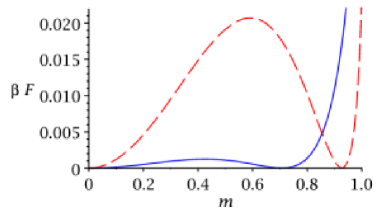
Figure 12: (Color online) Mean-field free energy for model (16) at the transition temperature, for $p=1$ (Ising-$\mathbb{R}P^{3}$ model, solid line) and $p=2$ (dashed line). In both cases there are two stable mean-field solutions and the transition is first order. However the energy barrier is much smaller for $p=1$.

We also mention that similar conclusions can be made for model (14) with $a=1.75$.

Once again, these results support our claim that the Ising-$\mathbb{R}P^{3}$ model is close to a point in parameter space where the transition changes from first to second order, in qualitative agreement with the simulation results.

VII Conclusion

We have proposed a minimal Ising-$\mathbb{R}P^{3}$ model that captures most of the low energy features of frustrated Heisenberg models with an $O(3)-$manifold of ground states. The discrete symmetry-breaking associated with the existence of two connected components of $O(3)$ leads to an Ising-type continuous transition with unconventional features at small sizes. The complexity of this transition is due to the strong coupling of the Ising chirality fluctuations to short range continuous spin fluctuations and to the topological defects of these textures.

We provided a consistent picture of these $\mathbb{Z}_{2}$ defects in presence of chiral fluctuations. Namely, we showed that chiral domain walls can also carry a $\mathbb{Z}_{2}$ topological charge, albeit delocalized over the interface. Inspection of configurations revealed that isolated vortex cores are almost always located nearby charged domain walls. At the transition temperature, most defects consist in vortex/charged-wall pairs, while there are a few vortex/vortex pairs and almost no isolated defect. This mechanism is essential in understanding the appearance of point defects at a temperature much lower than in the case where chiral fluctuations are absent.

We also studied some variants of the model and showed that the continuous transition easily becomes first-order, which lead us to conjecture the existence of a nearby tricritical point in parameter space. We clarified the role of short-range fluctuations of the continuous variables in this mechanism by an analogy with the large $q$-state Potts model. In this analogy the high density of states with orthogonal 4D-vectors translate into the large number $q(q-1)$ of states with disordered bonds of the Potts model. Finally we studied two derived versions of the original model: i) a diluted-Ising model, which somehow corresponds to a coarse-grained version of the Ising-$\mathbb{R}P^{3}$ model (the continuous variables are locally averaged and replaced by discrete variables), and ii) an effective multispin Ising model, obtained by tracing out the vector spins, order by order in $\beta$ (up to $\beta^{8}$). These two models predict either a weakly first-order or a continuous transition, as well as the existence of a tricritical point.

This study sheds light on the large variety of behaviors reported for chiral phase transitions in frustrated spin systems. momoi97 ; cs04 ; domenge05 ; domenge08 In all these models, the chirality is an emergent variable more or less coupled to short-range spin fluctuations: in the $J_{1}-J_{3}$ model on the square lattice the chiral variable is the pitch of an helix, the coupling to the short range spin fluctuations is probably small and the transition appears to be clearly second-order and in the Ising universality class. cs04 In the cyclic 4-spin exchange model on the triangular lattice, the order parameter is a tetrahedron and the chiral variable is associated to the triple product of three of these four spins: the transition is probably very weakly first order. momoi97 ; momoi99 In the $J_{1}-J_{2}$ model on the kagomé lattice, the order parameter at $T=0$ is a cuboactedron, and the chiral variable is associated to the triple product of three of these twelve spins. The phase transition evolves from weakly to strongly first order when tuning the parameters towards a ferromagnetic-antiferromagnetic phase boundary at $T=0$: this can be understood in the light of the present work. Tuning the parameters towards the ferromagnetic phase frustrates the 12-sublattice N el order and favors short-range disorder and vortex formation. The associated increase in the entropy unbalance drives the transition from Ising to strongly first order, much in the same way as in Section IV.

On the technical side, this proximity of a tricritical point in parameter space evidences why simulations and experiences must be lead with great caution, a conclusion equally supported by recent work from the quite different standpoint of the non perturbative renormalisation group approach. dmt04

VIII Acknowledgments

We thank D. Huse for suggesting this work and B. Bernu, E. Brunet, R. Mosseri and V. Dotsenko for helpful discussions.

Appendix A Monte-Carlo Algorithm

In this section we detail the Wang-Landau algorithm Wang2001 ; Schulz2003 used to simulate model (2). This method consists in building the density of states $g(E)$ progressively, using successive Monte Carlo iterations. Elementary moves consist in rotations of vectors $\vec{v}_{i}$ as well as flips of chiralities $\sigma_{i}$. In the case where the chiralities are frozen (Section II.2) only the rotation movements are performed. For completeness we mention that the four-vectors $\vec{v}_{i}$ are sampled uniformly on $S^{3}$ using 3 random numbers ($r$, $\eta$ and $\nu$), independent and uniformly distributed in $[0,1]$, according to

$$v_{1}=\begin{cases}\sqrt{r}\cos(2\pi\eta)&\\ \sqrt{r}\sin(2\pi\eta)\\ \sqrt{1-r}\cos(2\pi\nu)&\\ \sqrt{1-r}\sin(2\pi\nu)\end{cases}$$ (33)

Starting from an initial guess $g(E)$, the acceptance of a trial flip/rotation is decided by a Metropolis rule

$$\Pi(o\rightarrow n)={\rm Min}\left(1,\frac{g(E_{o})}{g(E_{n})}\right)$$ (34)

where the subscripts $o$ and $n$ corresponds the old and new configurations, respectively.

Every time a configuration with energy $E$ is visited, the density of states $g(E)$ is multiplied by a factor $f>1$, $g(E)\leftarrow g(E)f$. To ensure that all configurations are well sampled, a histogram $H(E)$ accumulates all visited states. The first part of the run is stopped when $H(E)>10^{4}$. In a second part, the histogram $H(E)$ is reset and the run is continued, but the modification factor $f$ is now decreased to $f_{1}<f$. In the original paper by Wang, Wang2001 $f_{1}$ was taken as $\sqrt{f}$, but this choice is not necessarily the best for continuous models. Poulain2006 In this case the convergence properties were found to be quite satisfying upon choosing $f_{1}=f^{0.7}$. The random walk is continued until the histogram of visits $H(E)$ has become “flat”. Once again, $H(E)$ is reset and the modification factor is decreased to $f_{2}<f_{1}$, etc… Accurate density of states $g_{n}(E)$ are generally obtained at the $n$-th iteration, where $n$ is such that $f_{n}$ is almost 1 (typically $f_{n}-1\lesssim 10^{-8}$).

Since this model has continuous variables, its energy spectrum is also continuous, and the choice of the energy bin requires special care: if the bin is too large, important details of the spectrum may be lost, whereas if it is too small, a lot of computer time is wasted to ensure the convergence of the method. In the temperature range of interest, a size of order $\simeq 0.1$ is a good compromise for the model of Eq. 10. In addition, the energy range is limited to the region relevant at the transition, and yields all thermodynamic quantities accurately at these temperatures.

Once the density of states $g(E)$ is obtained, all moments of the energy distribution can be computed in a straightforward way as

$$\langle E^{n}\rangle=\frac{\int g(E)E^{n}\exp(-\beta E)}{\int g(E)\exp(-\beta E)}$$ (35)

from which the specific heat per site is readily obtained:

$$C_{v}=\frac{1}{N}\left(\langle E^{2}\rangle-(\langle E\rangle)^{2}\right).$$ (36)

For the thermodynamic quantities that are not directly related to the moments of the energy distribution, such as the chirality, the vorticity, and their associated susceptibilities, or the Binder cumulants, we proceed as follows: an additional simulation is performed where $g(E)$ is no longer modified (a “perfect” random walk in energy space if the density of states $g(E)$ is very accurate). In this last run additional histograms are stored: chirality histograms $\sigma(E)$, $\sigma^{2}(E)$, $\sigma^{4}(E)$, and vorticity histogram $V(E)$, $V^{2}(E)$, $V^{4}(E)$.

Chirality (or vorticity) moments are then obtained from the simple 1D integration

$$\langle M^{n}\rangle=\frac{\int g(E)\frac{M^{n}(E)}{H(E)}\exp(-\beta E)}{\int g(E)\exp(-\beta E)}$$ (37)

from which, say, the Binder cumulant, is readily obtained as

$$U=1-\frac{\langle M^{4}\rangle}{3(\langle M^{2}\rangle)^{2}}$$ (38)

where $M=\sigma$ or $V$. Contrary to the method of the Joint Density of States, Zhou2006 our method does not require the construction of the two dimensional histogram $g(E,\sigma)$. Hence it is not limited to modest lattice sizes (the above quantities are computed for $L$ up to $L=80$).

References

- (1) J. Villain, J. Phys. (Paris) 38, 385 (1977).
- (2) P. Chandra, P. Coleman, and A. I. Larkin, Phys. Rev. Lett. 64, 88 (1990).
- (3) C. Weber, L. Capriotti, G. Misguich, F. Becca, M. Elhajal and F. Mila, Phys. Rev. Lett. 91, 177202 (2003).
- (4) T. Momoi, K. Kubo, and K. Niki, Phys. Rev. Lett. 79, 2081 (1997).
- (5) L. Capriotti and S. Sachdev, Phys. Rev. Lett. 93, 257206 (2004)
- (6) J.-C. Domenge, P. Sindzingre, C. Lhuillier and L. Pierre, Phys. Rev. B 72, 024433 (2005).
- (7) J.-C. Domenge, C. Lhuillier, L. Messio, L. Pierre and P.Viot, Phys. Rev. B 77, 172413 (2008).
- (8) P. C. Hohenberg, Phys. Rev. 158, 383 (1967); N. D. Mermin and H. Wagner, Phys. Rev. Lett. 17, 1133 (1966).
- (9) Sooyeul Lee and Koo-Chul Lee, Phys. Rev. B 49, 15184 (1994). D. Loison and P. Simon, Phys. Rev. B 61, 6114 (2000).
- (10) E. Brézin and J. Zinn-Justin, Phys. Rev. Lett. 36, 691 (1976).
- (11) W. Maier and A. Saupe, Z. Naturforsh. A 14, 882 (1959). P. A. Lebwohl and G. Lasher, Phys. Rev. A 6, 426 (1972).
- (12) P. E. Lammert, D. S. Rokhsar and J. Toner, Phys. Rev. Lett. 70, 1650 (1993). P. E. Lammert, D. S. Rokhsar and J. Toner, Phys. Rev. E 52, 1778 (1995).
- (13) S. Caracciolo, R. G. Edwards, A. Pelissetto and A. D. Sokal, Phys. Rev. Lett. 71, 3906 (1993).
- (14) H. Kawamura and S. Miyashita, J. Phys. Soc. Jpn. 53, 4138 (1984).
- (15) G. Kohring and R. E. Shrock, Nucl. Phys. B 285, 504 (1987).
- (16) T. Dombre and N. Read, Phys. Rev. B 39, 6797 (1989).
- (17) P. Azaria, B. Delamotte, and T. Jolicoeur, Phys. Rev. Lett. 64, 3175 (1990).
- (18) H. Kunz and G. Zumbach, Phys. Rev. B 46, 662 (1992).
- (19) P. Azaria, B. Delamotte, T. Jolicoeur, and D. Mouhanna, Phys. Rev. B 45, 12612 (1992).
- (20) B. W. Southern and A. P. Young, Phys. Rev. B 48, 13170 (1993).
- (21) B. W. Southern and H.-J. Xu, Phys. Rev. B 52, R3836 (1995).
- (22) M. Hasenbusch, Phys. Rev. D 53, 3445 (1996).
- (23) M. Wintel, H. U. Everts and W. Apel, Phys. Rev. B 52, 13480 (1995).
- (24) M. Caffarel, P. Azaria, B. Delamotte, and D. Mouhanna, Phys. Rev. B 64, 014412 (2001).
- (25) N. D. Mermin, Rev. Mod. Phys. 51, 591 (1979).
- (26) T. Momoi, H. Sakamoto, K. Kubo, Phys. Rev. B 59, 9491 (1999).
- (27) E. Domany, M. Schick, and R. H. Swendsen, Phys. Rev. Lett. 52, 1535 (1984).
- (28) H. W.J. Blote, W. Guo, and H. J. Hilhorst, Phys. Rev. Lett. 88, 047203 (2002).
- (29) A. C. D. van Enter and S. B. Shlosman, Phys. Rev. Lett. 89, 285702 (2002).
- (30) R. J. Baxter, J. Phys. C 6, L 445 (1973).
- (31) B. Nienhuis, A. N. Berker, E. K. Riedel and M. Schick, Phys. Rev. Lett. 43, 737 (1979).
- (32) M. Blume, Phys. Rev. 141, 517 (1966); H. W. Capel, Physica 32 966, (1966).
- (33) O. G. Mouritsen, S. J. Knak Jensen, B. Frank, Phys. Rev. B 24, 347 (1981); O. G. Mouritsen, B. Frank and D. Mukamel, Phys. Rev. B 27, 3018 (1983).
- (34) J. Oitmaa and R. W. Gibberd, J. Phys. C: Solid State Phys. 6, 2077 (1973).
- (35) J. Oitmaa, J. Phys. C: Solid State Phys. 7, 389 (1974).
- (36) M. Gitterman and M. Mikulinski, J. Phys. C: Solid State Phys. 10, 4073 (1977).
- (37) B. Delamotte, D. Mouhanna and M. Tissier, Phys. Rev. B 69, 134413 (2004).
- (38) F. W. Wang and D. P. Landau, Phys. Rev. Lett. 86, 2050 (2001).
- (39) B. J. Schulz, K. Binder, M. Muller and D. P. Landau, Phys. Rev. E 67, 067102 (2003).
- (40) P. Poulain, F. Calvo, R. Antoine, M. Broyer and Ph. Dugourd, Phys. Rev. E 73, 056704 (2006).
- (41) C. Zhou, T. C. Schulthess, S. Torbrugge and D. P. Landau, Phys. Rev. Lett. 96, 120201 (2006). J. Phys. A 9, 2125 (1976).