The Lagrangian-averaged model for magnetohydrodynamics turbulence and the absence of bottleneck

Abstract

We demonstrate that, for the case of quasi-equipartition between the velocity and the magnetic field, the Lagrangian-averaged magnetohydrodynamics $\alpha-$model (LAMHD) reproduces well both the large-scale and small-scale properties of turbulent flows; in particular, it displays no increased (super-filter) bottleneck effect with its ensuing enhanced energy spectrum at the onset of the sub-filter-scales. This is in contrast to the case of the neutral fluid in which the Lagrangian-averaged Navier-Stokes $\alpha-$model is somewhat limited in its applications because of the formation of spatial regions with no internal degrees of freedom and subsequent contamination of super-filter-scale spectral properties. We argue that, as the Lorentz force breaks the conservation of circulation and enables spectrally non-local energy transfer (associated to Alfvén waves), it is responsible for the absence of a viscous bottleneck in MHD, as compared to the fluid case. As LAMHD preserves Alfvén waves and the circulation properties of MHD, there is also no (super-filter) bottleneck found in LAMHD, making this method capable of large reductions in required numerical degrees of freedom; specifically, we find a reduction factor of $\approx 200$ when compared to a direct numerical simulation on a large grid of $1536^{3}$ points at the same Reynolds number.

I Introduction

When large-scale numerical simulations of astrophysical or geophysical magnetohydrodynamics (MHD) are desired, all dynamical scales of the physical system are rarely, if ever, resolved. For this reason, sub-grid-scale (SGS) modeling of MHD dynamics in the context of computations in the geophysical and astrophysical context is required. This modeling can be achieved implicitly, in the simplest example by employing a dissipative numerical scheme, or it can be done explicitly by creating a Large Eddy Simulation (LES–see MK00 for a recent review). Explicit methods for MHD are not as pervasive as they are in engineering, or for geophysical and atmospheric flows. In fact, modeling for MHD is a relatively new field (see PFL76 ; Y87 ). One problem with extending the LES methodology for hydrodynamic turbulence to MHD is that most LES are based upon eddy-viscosity concepts MK00 , which can be related to a known power law of the energy spectrum ChLe1981 (although generalizations can be devised, see e.g. BaPoPo+2008 ), or upon self-similarity. For MHD, the underlying assumption of locality of interactions in Fourier space is not necessarily valid AMP05a ; MAP05 (a contradiction of self-similarity) and spectral eddy-viscosity concepts ZSG02 cannot be applied in a straightforward manner as neither kinetic nor magnetic energy is a conserved quantity and the general expression of the energy spectrum is not known at this time I64 ; K65 ; GoSr1995 ; GaNaNe+2000 ; MiPo2007a ; PoMiMo+2008 ; MaCaBo2008 . Purely dissipative models TFS94 ; AMK+01 are inadequate as they ignore the exchange of energy at sub-filter scales between the velocity and magnetic fields and such models have been shown to suppress small-scale dynamo action HB06 and any inverse cascade from the sub-filter scales MC02 . A satisfactory LES for MHD has been proposed for the case starting with some degree of alignment between the velocity and magnetic fields LS91 ; MC02 . Other restricted-case MHD-LES are applicable to low magnetic Reynolds number PPP04 ; KM04 ; PMM+05 . Extensions of spectral models to MHD based on two-point closure formulations of the dynamical equations proposed recently look promising in the analysis of turbulent flows and of the dynamo mechanism BaPoPo+2008 . Finally, though technically not an LES, there are also hyper-resistive models for MHD which require rescaling of the length (wavenumber) scales to a known direct numerical simulation (DNS) HB06 .

One model which can be written as an LES is the Lagrangian-averaged MHD (LAMHD) equations H02a ; H02b ; MP02 . It has been shown to reproduce a number of features of DNS. In two dimensions (2D) for Taylor Reynolds numbers ($R_{\lambda}$) up to $\approx 5000$ it has been shown to reproduce selective decay, the inverse cascade of mean-square vector potential, and dynamic alignment between the velocity and magnetic fields MMP05a as well as the statistics of small-scale cancellation PGMP05 and intermittency PGHM+06 . In three dimensions (3D) at Reynolds numbers ($Re$) of $\approx 500$, LAMHD reproduced the inverse cascade of magnetic helicity (associated with the development of force-free magnetic field) and the helical dynamo effect MMP05b . It has also been tested (up to kinetic $Re\approx 3000$, magnetic $Re\approx 300$) for its ability to predict the critical magnetic Reynolds number for a non-helical dynamo at low magnetic Prandtl number Mi2006a . LAMHD performed well in all these tests. Its equivalent hydrodynamic model, the Lagrangian-averaged Navier-Stokes (LANS) equations, also performed well in tests at $R_{\lambda}\lessapprox 300$ (see CHO+05 and references in PGHM+07a ). However, above $Re\approx 3000$ ($R_{\lambda}\approx 800$), it was shown that placing the filter width in the inertial range leads to contamination of the super-filter-scale properties (such as the spectra) for LANS. We refer here to this effect as the super-filter-scale bottleneck, which may be different in nature from the viscous bottleneck observed in some DNS of the Navier-Stokes equations. The contamination may be linked to the formation of spatial regions in the flow with no internal degrees of freedom (so-called “rigid bodies”) PGHM+07a , which also correspond to the development of a secondary inertial range of the LANS equations at sub-filter scales. This super-filter-scale contamination provides an effective constraint on the filter size and, hence, on the available reduction of the total number of the (numerical) degrees of freedom ($N_{dof}$) needed to reproduce the large-scale dynamics of the flow at a given Reynolds number; a factor of $\approx 10$ can be achieved. This limitation is not apparent in low and moderate Reynolds number (resolution) simulations (e.g., $64^{3}$ LANS compared with $256^{3}$ DNS) as the scale separation is not enough for the above-mentioned phenomenon of contamination of small-scale spectra because of rigid body regions in the flow to appear. The bottleneck (and super-filter-scale contamination) was not studied as such but neither was it observed in 2D LAMHD for high Reynolds number MMP05a ; PGMP05 ; PGHM+06 . 3D LAMHD has only been tested at more moderate Reynolds number MMP05b (see also MiPoSu2008 for a recent review). The aim of the present work is, thus, to determine if LAMHD in three space dimensions, for higher Reynolds number develops problems similar to that of LANS. Specifically, we test for the existence of spatial regions with no available internal degrees of freedom. We show in the following that LAMHD behaves better in this respect than LANS, and, thus, continues to appear as a promising model for MHD flows.

II The equations of motion

We consider the incompressible MHD equations for a fluid with constant density,

$$\partial_{t}\mathbf{v}+\bm{\omega}\times\mathbf{v}=\mathbf{j}\times\mathbf{b}-\bm{\nabla}p+\nu\nabla^{2}\mathbf{v}$$

$$\partial_{t}\mathbf{b}=\bm{\nabla}\times\left(\mathbf{v}\times\mathbf{b}\right)+\eta\nabla^{2}\mathbf{b}$$

$$\bm{\nabla}\cdot\mathbf{v}=\bm{\nabla}\cdot\mathbf{b}=0,$$ (1)

where $\mathbf{v}$ and $\mathbf{b}$ denote respectively the velocity and magnetic fields, $p$ the pressure divided by the density, $\nu$ the kinematic viscosity, and $\eta$ the magnetic diffusivity. As is well known, in incompressible MHD, Alfvén waves will travel along a uniform background field, $\mathbf{b}_{0}$. From linear perturbation analysis the dispersion relation between wavenumber, $k$, and frequency, $\omega$, is

$$\left(\omega+i\eta k^{2}\right)\left(\omega+i\nu k^{2}\right)=k^{2}b_{0}^{2}\,.$$ (2)

The wave speed is $|\mathbf{b}_{0}|$ and, assuming $\eta=\nu$, the amplification factor is given by $\exp(-\eta k^{2}t)$. The ideal ($\eta=\nu=0$) quadratic invariants for MHD are in the $L^{2}$ norm. For example, the total energy is given by:

$$E_{T}=\frac{1}{2}\left(||v||_{2}+||b||_{2}\right)\equiv\frac{1}{2}\frac{1}{D}\int_{D}\left(|\mathbf{v}|^{2}+|\mathbf{b}|^{2}\right)d^{3}x.$$ (3)

The LAMHD equations H02a are given by

$$\partial_{t}\mathbf{v}+\bm{\omega}\times\mathbf{u}=\mathbf{j}\times\bar{\mathbf{b}}-\bm{\nabla}\Pi+\nu\nabla^{2}\mathbf{v}$$

$$\partial_{t}\bar{\mathbf{b}}=\bm{\nabla}\times\left(\mathbf{u}\times\bar{\mathbf{b}}\right)+\eta\nabla^{2}\mathbf{b}$$

$$\bm{\nabla}\cdot\mathbf{v}=\bm{\nabla}\cdot\mathbf{u}=\bm{\nabla}\cdot\mathbf{b}=\bm{\nabla}\cdot\bar{\mathbf{b}}=0,$$ (4)

where $\mathbf{u}$ ($\bar{\mathbf{b}}$) denotes the filtered component of the velocity (magnetic) field and $\Pi$ the modified pressure. Filtering is accomplished by the application of a normalized convolution filter $L:f\mapsto\bar{f}$ where $f$ is any scalar or vector field. By convention, we define $\mathbf{u}\equiv\bar{\mathbf{v}}$. LAMHD in the form given in Eqs. (4) is both computationally efficient and makes clear that Alfvén’s theorem is preserved by the model: the smoothed magnetic field is advected by the smoothed velocity. In the remainder of this paper, we take $\eta=\nu$ (unit magnetic Prandtl number) and, thus, it is sufficient to introduce the same filtering for the velocity and magnetic fields in this case. This allows us to write LAMHD in LES form,

$$\partial_{t}\mathbf{u}+\bar{\bm{\omega}}\times\mathbf{u}=\bar{\mathbf{j}}\times\bar{\mathbf{b}}-\bm{\nabla}\bar{\Pi}+\nu\nabla^{2}\bar{\mathbf{v}}-\mathbf{\nabla}\cdot\bar{\tau}$$

$$\partial_{t}\bar{\mathbf{b}}=\bm{\nabla}\times\left(\mathbf{u}\times\bar{\mathbf{b}}\right)+\eta\nabla^{2}\bar{\mathbf{b}}-\mathbf{\nabla}\cdot\bar{\tau}^{b}$$

$$\bm{\nabla}\cdot\mathbf{v}=\bm{\nabla}\cdot\mathbf{u}=\bm{\nabla}\cdot\mathbf{b}=\bm{\nabla}\cdot\bar{\mathbf{b}}=0.$$ (5)

We choose as our filter the inverse of a Helmholtz operator, $L=\mathcal{H}^{-1}=(1-\alpha^{2}\nabla^{2})^{-1}$. Therefore, $\mathbf{u}=g_{\alpha}\otimes\mathbf{v}$ where $g_{\alpha}$ is the Green’s function for the Helmholtz operator, $g_{\alpha}(r)=\exp(-r/\alpha)/(4\pi\alpha^{2}r)$ (i.e., the Yukawa potential), or in Fourier space, $\hat{\mathbf{u}}(k)=\hat{\mathbf{v}}(k)/(1+\alpha^{2}k^{2})$. The effective filter width is, thus, approximately $\alpha$. With this choice, the Reynolds (turbulent) SGS stress tensor is given by

$$\bar{\tau}=\alpha^{2}\left(\mathbf{\nabla}\mathbf{u}\cdot\mathbf{\nabla}\mathbf{u}^{T}+\mathbf{\nabla}\mathbf{u}\cdot\mathbf{\nabla}\mathbf{u}-\mathbf{\nabla}\mathbf{u}^{T}\cdot\mathbf{\nabla}\mathbf{u}-\mathbf{\nabla}\bar{\mathbf{b}}\cdot\mathbf{\nabla}\bar{\mathbf{b}}^{T}-\mathbf{\nabla}\bar{\mathbf{b}}\cdot\mathbf{\nabla}\bar{\mathbf{b}}+\mathbf{\nabla}\bar{\mathbf{b}}^{T}\cdot\mathbf{\nabla}\bar{\mathbf{b}}\right)$$ (6)

and the divergence of the electromotive-force (emf) SGS stress tensor by

$$\mathbf{\nabla}\cdot\bar{\tau}^{b}=\eta\alpha^{2}\nabla^{4}\bar{\mathbf{b}}.$$ (7)

In this form, the expression of the SGS tensors make explicit the fact that $\mathbf{u}=\pm\bar{\mathbf{b}}$ Alfvén waves are preserved even in the subgrid scales. These $\mathbf{u}=\pm\bar{\mathbf{b}}$ waves travel along $\bar{\mathbf{b}}_{0}$ (the smoothed and unsmoothed fields are identical for uniform ${\mathbf{b}}_{0}$) and the dispersion relation is

$$\left(\omega+i\nu k^{2}\right)\left(\omega+i\eta k^{2}(1+\alpha_{M}^{2}k^{2})\right)=k^{2}\bar{b}_{0}^{2}\frac{1+\alpha_{M}^{2}k^{2}}{1+\alpha_{K}^{2}k^{2}}\,,$$ (8)

where $\alpha_{K}$ and $\alpha_{M}$ are the filter widths for the smoothing of the velocity and magnetic fields, respectively. For $\alpha\equiv\alpha_{K}=\alpha_{M}$ and $\eta=\nu$ (the case we study), the wave speed is given by $\bar{\mathbf{b}}_{0}{\left(1-(\eta k\alpha^{2}k^{2}/\bar{b}_{0})^{2}/8+\mathcal{O}((\eta k\alpha^{2}k^{2}/\bar{b}_{0})^{6})\right)}$, the strength of the smoothed background magnetic field reduced by an order $\alpha^{4}k^{4}$ term. The amplification factor is given by $\exp\left(-\eta k^{2}t(1+\alpha^{2}k^{2}/2)\right)$ for both $u=-\bar{b}$ waves traveling in the direction of $\bar{\mathbf{b}}_{0}$ and $u=\bar{b}$ waves traveling anti-parallel to $\bar{\mathbf{b}}_{0}$. Finally, the ideal quadratic invariants for LAMHD are in the $H^{1}_{\alpha}(\bar{f})$ norm. For example, the total energy is given by a mixture of the smooth and rough fields, namely:

$$E_{T}^{\alpha}=\frac{1}{2}\left(||u||_{2}^{\alpha}+||\bar{b}||_{2}^{\alpha}\right)\equiv\frac{1}{2}\frac{1}{D}\int_{D}\left(\mathbf{u}-\alpha^{2}\nabla^{2}\mathbf{u}\right)\cdot\mathbf{u}+\left(\bar{\mathbf{b}}-\alpha^{2}\nabla^{2}\bar{\mathbf{b}}\right)\cdot\bar{\mathbf{b}}~{}d^{3}x$$

$$=\frac{1}{2}\frac{1}{D}\int_{D}\mathbf{v}\cdot\mathbf{u}+\mathbf{b}\cdot\bar{\mathbf{b}}~{}d^{3}x.$$ (9)

We solve both sets of equations, Eqs. (1) and (4), for one specific instance of a decaying MHD flow, using a parallel pseudospectral code GMD05 ; GMD05b in a three-dimensional (3D) cube with periodic boundary conditions. The initial conditions for the velocity and magnetic fields are constructed from a superposition of three Beltrami (helical) ABC flows to which smaller-scale random fluctuations are added with initial kinetic and magnetic energy $E_{K}=E_{M}=0.5$, magnetic helicity $H_{M}=<\mathbf{a}\cdot\mathbf{b}>\approx 0.45$ ($\mathbf{b}=\mathbf{\nabla}\times\mathbf{a}$ where $\mathbf{a}$ is the vector potential and the brackets denote volume average), and the initial co-alignment of the fields, $\left<\mathbf{v}\cdot\mathbf{b}\right>\left<|\mathbf{v}||\mathbf{b}|\right>^{-1}\approx 10^{-4}$ (see MiPoMo2006 ; MiPo2007a for details). A MHD-DNS with a resolution $N^{3}=1536^{3}$ (i.e., 1536 grid points in real space in each direction) and $\eta=\nu=2\cdot 10^{-4}$ is used as our high Reynolds number test case for the LAMHD model. The DNS computation is stopped when the growth of the total dissipation begins to enter the saturation phase ($t=3.7$), at which time the Reynolds number based on the mechanical integral scale is $Re\approx 9200$ and the Taylor Reynolds number $\approx 1100$. The MHD flow resulting from the initial conditions employed has previously been analyzed for its spectral properties and for the spatial structures it develops MiPoMo2006 ; MiPo2007a ; MaPoMi+2008 . In this paper, we perform a simulation with similar initial conditions and parameters but now using LAMHD at a resolution of $512^{3}$ grid points; we also perform for comparison purposes a Navier-Stokes LANS run with the same initial velocity field but with $\mathbf{b}\equiv 0$, on a grid of $512^{3}$ points. In both cases, the filter width is $\alpha=2\pi/18$ ($k_{\alpha}=18$) and is, thus, large enough to preclude any artifact of numerical resolution altering the results. Based on previous analyses FHT01 ; PGHM+07a , we estimate ${k_{max}}/{k_{\eta}^{\alpha}}\approx 2.4$ (where $k_{max}$ is the maximum wavenumber resolved in the simulation, and $k_{\eta}^{\alpha}$ is the LAMHD dissipation scale) using computations conducted for $\eta=\nu=6\cdot 10^{-4}$ with a Reynolds number of $Re\approx 2200$. However, the main point of using such a large filter is to test if LAMHD fails in the same way as LANS. We finally perform a LES simulation in a $256^{3}$ grid using the LAMHD equations with the same viscosity and diffusivity as the $1536^{3}$ DNS used for the comparison. In this way, we extend the $Re\approx 9200$ computation in time by a factor of 3.

III Results

III.1 Spectral contamination in LANS  for an ABC flow and its absence in the MHD case

One of the main findings of our preceding work with LANS on the Navier-Stokes equations is that a $k^{+1}$ scaling develops in the (kinetic) energy spectrum at sub-filter scales; this leads to a contamination of super-filter scales because of detailed energy conservation (per triadic interactions). This LANS $k^{+1}$ spectrum (together with super-filter-scale spectral contamination) has only recently been recognized, in the case of one specific forcing function at large Reynolds number PGHM+07a , but such a spectral contamination has not yet been generally demonstrated (although theoretical arguments for the $k^{+1}$ spectrum have been given in PGHM+07a ). Thus, we first confirm its presence in a LANS simulation with the same viscosity and the (nearly) same initial conditions for the velocity field as for the MHD-DNS (and LAMHD runs) examined in this paper, and based on large-scale ABC flows with superimposed random noise at small scale. Due to the presence of random noise and considering the differences in resolution and the presence of a filter in the LAMHD runs, the initial conditions were not exactly reproduced, although the same procedure was used to generate them. In the present Navier-Stokes case, we find again what can be called an enhanced (super-filter-scale) bottleneck: the positive power-law spectral contamination of the kinetic energy spectrum $E_{K}(k)$ in the LANS run is observed for times after the peak of dissipation (see dotted line, Fig. 1a). The fitted spectrum is $k^{+0.5}$ (note that $k^{+1}$ requires the entire LANS spectrum to be resolved, and therefore has only been observed for much larger values of ${k_{max}}/{k_{\eta}^{\alpha}}$).

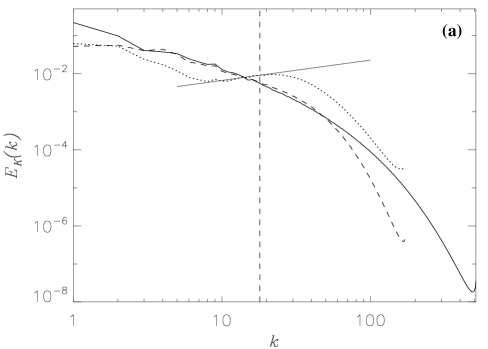
Figure 1: (a) Spectra of kinetic energy (normalized to DNS $E_{K}(14)$, see text) for $1536^{3}$ MHD DNS (solid line), $512^{3}$ LAMHD (dashed), and $512^{3}$ LANS (dotted), in the latter case with ${\bf b}\equiv 0$ at all times but otherwise identical conditions. For intermediate scales, $k\in[5,40]$, LAMHD reproduces the scaling of the DNS, the larger scales being affected by slight differences in initial conditions, see text. For $k$ close to the filter scale ($k\in[k_{\alpha}/2,k_{\alpha}]$), a positive power law, $k^{0.5}$ (gray line), is found for LANS. (b) Spectra of magnetic energy (normalized to DNS $E_{M}(14)$) for the same runs: LAMHD reproduces the scaling of the DNS even beyond the filter wavenumber, $k_{\alpha}=18$ as indicated by the vertical dashed line. LAMHD exhibits neither the positive power-law nor the super-filter-scale spectral contamination associated with high Reynolds number LANS modeling seen in (a).

For the given parameters and initial conditions, we find the super-filter-scale bottleneck for LANS. However, when integrating the MHD equations with the Lagrangian model (dashed line, Fig. 1a) with these same parameters, no such contamination is present. Note that the spectra for the DNS-MHD are shown at the time of peak dissipation, while the spectra for the Lagrangian-averaged models are for a slightly later time in order to allow for the possible formation of rigid bodies, which are known to be at the source of the spectral contamination close to the filter wavenumber in the Navier-Stokes case. For this reason, and due to the slight differences in initial conditions, we have chosen to plot spectra normalized to that of the DNS at $k=14$ to emphasize the scaling. For most of the inertial range (also in an approximate sense below the filter width $\alpha$) the scaling of $E_{K}(k)$ is reproduced by the LAMHD simulation. The sub-filter scaling for LAMHD is not as steep as MHD, but is not a positive scaling law. The agreement for $E_{M}(k)$ is remarkable. More importantly, neither positive-power-law spectra nor contamination of the super-filter-scale spectra are evidenced at all.

III.2 The lack of rigid bodies in LAMHD  in the large$-\alpha$ limit for unforced flows

Evidence for the development of rigid bodies in LANS (which led to its limited use as a LES) has only been shown for $l\ll\alpha$ PGHM+07a . Since investigation of the large$-\alpha$ limit is not as computationally demanding as the small$-l$ limit, it is interesting to look at this limit as a rough indication of what occurs for small $\alpha$ and smaller $l$. This approach has been employed both for the LANS Navier-Stokes case in two dimensions LKT+07 and in three dimensions PGHM+07a . In such a case, the purpose is to examine the properties of the model itself, as opposed to trying to reproduce large-scale properties, the large-scale behavior being reduced to a very small span of wavenumbers. With this practice, the properties of the sub-filter-scales can be studied, to better understand the origin (or lack) of super-filter-scale contamination. We now use this limit to further explore the differences between LAMHD and LANS. We employ simulations for the two models with the same initial conditions as before, with $\eta=\nu=5\cdot 10^{-5}$ ($Re\approx 26,000$ at peak of dissipation for LAMHD), and a resolution of $256^{3}$ grid points. Note that these dissipative coefficients are four times smaller than what was considered in the previous section since, for a fixed resolution, the achievable Reynolds number goes as $\alpha^{2/3}$. This follows for LANS from the predicted (and verified) degrees of freedom, $N^{\alpha}_{dof}\propto\alpha^{-1}Re^{3/2}$ FHT01 ; PGHM+07a . The scaling of LAMHD may differ, but the same value of the viscosity is employed for the two models, regardless.

For LANS, we observe the expected $k^{+1}$ zero flux inertial range (see Fig. 2) which is followed by a viscous (sub-filter-scale) bottleneck feature, $k^{+1.5\pm.2}$, before the dissipative range proper. We conducted a second simulation with $\nu=10^{-4}$ and found a $k^{1.4\pm.3}$ spectrum. This is analogous to results for DNS of the Navier-Stokes equations where only the viscous bottleneck is observed at moderate Reynolds number and is preceded by an inertial range only for higher Reynolds. These viscous bottlenecks may be different in nature from the (super-filter-scale) bottlenecks discussed before, which are not associated to the onset of the dissipative range but to the development of a secondary inertial range in LANS below the filtering length, and result in contamination of the large (resolved) scales when the LANS equations are used as an LES. Having confirmed that our analysis from the forced LANS case extends to the decaying LANS simulation, we now apply it to LAMHD. The large$-\alpha$ LAMHD spectra are given in Fig. 3. Notably, there is no positive-power-law spectrum.

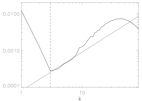
Figure 2: Spectrum of kinetic energy for a $256^{3}$ grid with $k_{\alpha}=3$ ($\nu=5\cdot 10^{-5}$) LANS, ${\bf b}\equiv 0$ (Navier-Stokes case). The fitted grey line, $k^{+1.1\pm.4}$, agrees with the rigid-body hypothesis for the inertial range PGHM+07a . This slope is followed by a steeper slope attributed to a bottleneck, with $k^{+1.5\pm.2}$.

Predictions of energy spectra in the inertial range follow from the global scaling laws for third-order structure functions for isotropic, homogeneous turbulence. Exact results for these structure functions have been found for incompressible MHD PP98b and for LAMHD PGHM+06 . The latter are, in terms of both the smooth fields ${\bar{\bf z}}^{\pm}\equiv\mathbf{u}\pm\bar{\mathbf{b}}$ and the rough fields $\mathbf{z}^{\pm}\equiv\mathbf{v}\pm\mathbf{b}$ (where the z-fields are called the Elsässer variables):

$$\left<\delta\bar{z}_{\|}^{\mp}(\mathbf{l})\delta\bar{z}_{i}^{\pm}(\mathbf{l})\delta{z}_{i}^{\pm}(\mathbf{l})\right>\sim\varepsilon_{\pm}^{\alpha}l\ ,$$ (10)

where $\left<.\right>$ denotes volume averaging, $\delta f(\mathbf{l})\equiv f(\mathbf{x}+\mathbf{l})-f(\mathbf{x})$, and $\delta f_{\|}(\mathbf{l})\equiv\left[\mathbf{f}(\mathbf{x}+\mathbf{l})-\mathbf{f}(\mathbf{x})\right]\cdot\mathbf{l}$. For sub-filter scales ($l\ll\alpha$), $\bar{z}^{\pm}\sim l^{2}\alpha^{-2}{z}^{\pm}$ and the scaling law becomes dimensionally $\bar{z}z\bar{z}\sim\varepsilon l$. This implies a sub-filter scale spectrum corresponding to the invariants $E_{\pm}^{\alpha}\equiv||\bar{\mathbf{z}}^{\pm}||^{2}_{\alpha}/2$ for the ideal non-dissipative case. We then have $E^{\alpha}_{\pm}(l)k\sim z^{\pm}\bar{z}^{\pm}\sim(\varepsilon_{\pm}^{\alpha})^{2/3}\alpha^{2/3}$ or, equivalently,

$$E^{\alpha}_{\pm}(k)\sim(\varepsilon_{\pm}^{\alpha})^{2/3}\alpha^{2/3}k^{-1}$$ (11)

as for LANS FHT01 . Recall that in the flux relation, Eq. (10), $\varepsilon_{\pm}^{\alpha}$ stands for the energy transfer and dissipation rate of $E_{\pm}^{\alpha}$. Hence, the prediction, Eq. (11), for the spectra, $E^{\alpha}_{\pm}(k)$, is, equivalently for $E_{T}^{\alpha}\equiv(||u||^{2}_{\alpha}+||b||^{2}_{\alpha})/2$ and for $H_{C}^{\alpha}\equiv\frac{1}{2}\frac{1}{D}\int_{D}\mathbf{v}\cdot\bar{\mathbf{b}}~{}d^{3}x$. The spectra shown in Fig. 3 for large$-\alpha$ LAMHD do not exclude, due to the large uncertainties of the fitted power laws, the predicted $k^{-1}$ spectra.

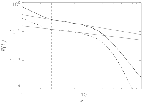
Figure 3: Spectra for a $256^{3}$ grid with $k_{\alpha}=3$ ($\eta=\nu=5\cdot 10^{-5}$) LAMHD, $Re\approx 26,000$: Total energy, $E_{T}(k)$, (solid line) and cross helicity, $H_{C}(k)$, (dashed). The fitted slopes, $E_{T}(k)\sim k^{-0.7\pm.3}$ and $H_{C}(k)\sim k^{-0.5\pm.4}$ could agree with either Kolmogorov or IK predictions for LAMHD (see text) at this level of uncertainty.

A spectral prediction for LAMHD can also be arrived at by dimensional analysis of the spectrum which follows the scaling ideas originally due to Kraichnan K67 and which is developed for LANS in Ref. CHT05 . Here, the energy dissipation rate, $\varepsilon^{\alpha}_{\pm}=dE^{\alpha}_{\pm}/dt$, is related to the spectral energy density by

$$\varepsilon^{\alpha}_{\pm}\sim(\mathfrak{t}_{k})^{-1}\int E^{\alpha}_{\pm}(k)$$ (12)

where $\mathfrak{t}_{k}$ is the turnover time for an eddy of size $\sim k^{-1}$. This turnover time is related to a “velocity,” $\bar{Z}_{k}^{\pm}$, (i.e., $\mathfrak{t}_{k}\sim 1/(k\bar{Z}_{k}^{\pm})$), where $(\bar{Z}_{k}^{\pm})^{2}\sim\bar{Z}_{k}^{\pm}{Z}_{k}^{\pm}/(1+\alpha^{2}k^{2})\sim kE^{\alpha}_{\pm}(k)/(1+\alpha^{2}k^{2})$. Substitution into Eq. (12) yields,

$$E^{\alpha}_{\pm}(k)\sim(\varepsilon^{\alpha}_{\pm})^{2/3}k^{-5/3}(1+\alpha^{2}k^{2})^{1/3}$$ (13)

or, for $\alpha k\gg 1$,

$$E^{\alpha}_{\pm}(k)\sim(\varepsilon^{\alpha}_{\pm}\alpha)^{2/3}k^{-1}.$$ (14)

In the Iroshnikov-Kraichnan I64 ; K65 (hereafter, IK) phenomenology, Alfvén waves (corresponding to either $z^{\mp}=0$) can only interact nonlinearly when they collide along field lines (along which they travel in opposite directions). The characteristic time for an Alfvén wave is $\mathfrak{t}_{A}\sim(kB_{0})^{-1}$. If this is less than $\mathfrak{t}_{k}$, the effective transfer time $\mathfrak{t}_{T}$ is increased, $\mathfrak{t}_{T}\sim\mathfrak{t}_{k}^{2}/\mathfrak{t}_{A}$. Substitution of this new transfer time into Eq. (12) yields, instead of Eq. (13)

$$E^{\alpha}_{\pm}(k)\sim(\varepsilon^{\alpha}_{\pm}B_{0})^{1/2}k^{-3/2}(1+\alpha^{2}k^{2})^{1/2}$$ (15)

or, for $\alpha k\gg 1$,

$$E^{\alpha}_{\pm}(k)\sim(\varepsilon^{\alpha}_{\pm}B_{0})^{1/2}\alpha k^{-1/2}.$$ (16)

The spectra shown in Fig. 3 for large$-\alpha$ LAMHD also agree with the IK predicted spectra, Eq. (16). In fact, the spectra more closely correspond to this prediction; this is consistent with the fact that, for this flow, an IK spectrum $E(k)\sim k^{-3/2}$ is observed at large scale (followed by a weak turbulence anisotropic spectrum $E(k_{\perp})\sim k_{\perp}^{-2}$ at small scale) MiPo2007a . Again, simulations at higher resolution are needed for a definite answer and the result may not be universal as shown for example in the context of reduced MHD dynamics due to the presence of a strong uniform magnetic field ${\bf B}_{0}$ DmGoMa2003 or for MHD with a strong ${\bf B}_{0}$ MaCaBo2008 .

Figure 4: PDFs of cubed increments. The cubed increments when averaged are equal to flux times length, $\varepsilon^{\alpha}\cdot l$. Here $l=0.88\alpha$ ($\alpha=2\pi/3$). The dotted line is $\delta u_{\|}(l)\delta u_{i}(l)\delta v_{i}(l)$ for LANS, solid for LAMHD $\delta\bar{z}_{\|}^{-}(\mathbf{l})\delta\bar{z}_{i}^{+}(\mathbf{l})\delta{z}_{i}^{+}(\mathbf{l})$, and dashed for LAMHD $\delta\bar{z}_{\|}^{+}(\mathbf{l})\delta\bar{z}_{i}^{-}(\mathbf{l})\delta{z}_{i}^{-}(\mathbf{l})$. More of the volume gives no contribution to the flux for LANS than for LAMHD, indicating no rigid bodies in LAMHD.

Another indication of the zero-flux regions in LANS is found by examining the spatial variation of the cubed increments associated with the scaling laws $\delta u_{\|}(l)\delta u_{i}(l)\delta v_{i}(l)$ for LANS and $\delta\bar{z}_{\|}^{\mp}(\mathbf{l})\delta\bar{z}_{i}^{\pm}(\mathbf{l})\delta{z}_{i}^{\pm}(\mathbf{l})$ for LAMHD (note that one can transform this relation into the $u,\ v,\ b,\ {\bar{b}}$ variables). For a given length $l$, these cubed increments when averaged are related with the energy fluxes by Eq. (10) (the LANS relation and the hydrodynamic and MHD relations are contained in this expression in the corresponding limits). As a result of this correspondence, for brevity we will indicate cubed increments in the figures as the corresponding energy flux times the length used to compute the increments. This also allows us to identify regions with zero cubed increments as rigid bodies (a rigid rotation has zero longitudinal increments). Probability distribution functions (PDFs), see Fig. 4, indicate that LAMHD has a much smaller proportion of its volume, which could potentially be rigid bodies (i.e., frozen regions with no internal degrees of freedom (zero velocity increment), which therefore do not contribute to the energy flux). That is, more of the volume is contributing to the turbulent cascade. Snapshots for constructing the PDFs are taken from both $\alpha=2\pi/3$ Lagrangian-averaged models for times shortly after the peak of dissipation and when the LANS total dissipation is nearly equal to that of LAMHD. The strengths of the central peaks of the PDFs for large$-\alpha$ are another indication that LAMHD inherits none of the rigid-body or zero-flux-region problems of LANS.

III.3 Why are spectral properties of LAMHD  better than in the fluid case?

Why does LAMHD not exhibit the same spectral contamination as LANS? One possible cause is the hyperdiffusivity term seen in the LES form for LAMHD, Eq. (7), whereas there is no hyperviscosity-like term in LANS. To test if this hyperdiffusion is responsible for the lack of spectral contamination in LAMHD, we removed the hyperdiffusion by setting $\bar{\tau}^{b}=0$ in Eqs. (5) or, equivalently, by substituting $\eta\nabla^{2}\bar{\mathbf{b}}$ for $\eta\nabla^{2}\mathbf{b}$ in Eqs. (4). We then start the run from the same initial conditions but now with these new equations employing $\alpha=2\pi/33$ and $\nu=\eta=2\cdot 10^{-4}$ at a resolution of $384^{3}$ (with hyperdiffusion, a smaller resolution of $256^{3}$ is possible, see Section III.4). Note that such a modified LAMHD model is not expected to, nor found to, perform well as a SGS model; this numerical experiment is performed here only in order to assess the effect of the hyper-diffusive term introduced by the $\alpha$ modeling. We find that hyperdiffusion is not responsible for the lack of a $k^{+1}$ spectral contamination in LAMHD (see Fig. 5).

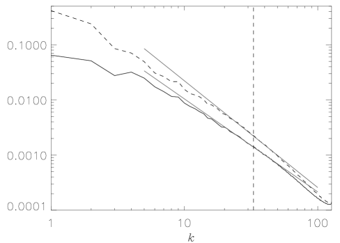
Figure 5: Spectra for a $384^{3}$ grid with $k_{\alpha}=33$ obtained from the modified-LAMHD (see text) shortly after the maximum of dissipation: kinetic energy (solid) and magnetic energy (dashed); the LAMHD equations have been modified by removing the hyperdiffusive turbulent emf. Even without hyperdiffusivity, no positive power-law is found. Instead, fits (grey lines) for kinetic and magnetic energy spectra near the filtering length are $k^{-1.7\pm.1}$ and $k^{-1.9\pm.1}$, respectively.

Other possible causes for LAMHD not exhibiting the super-filter-scale bottleneck as does LANS are the actual physical differences between the two fluids that are modeled, Navier-Stokes and MHD. First, unlike incompressible Navier-Stokes, MHD supports oscillatory solutions (Alfvén waves) which are linked to enhanced spectral nonlocality of energy transfer AMP05a ; Al2007a leading to dynamic interactions between widely separated scales. For Navier-Stokes, the depletion of energy transfer due to local interactions at some cutoff in wavenumber is believed to bring about the bottleneck effect HSL+82 ; LMG95 ; MCD+97 ; MAP06 . However, related to the spectrally nonlocal energy transfer via Alfvén waves, MHD does not seem to exhibit a bottleneck in its spectra between the inertial and dissipative ranges MiPo2007a . As LAMHD supports Alfvén waves at all scales (and alters their dissipation and wave speed appreciably only for sub-filter scales), the same physics could be behind the lack of a super-filter-scale bottleneck in LAMHD.

Another difference between the fluid and MHD cases is the geometry of the dissipative structures: one finds vortex filaments for Navier-Stokes at high value of the vorticity, and current and vorticity sheets for MHD; sheets which are found to roll-up at high Reynolds number MiPoMo2006 . It has been claimed that the development of helical filaments in the fluid case can lead to the depletion of nonlinearity and the quenching of local interactions MT92 ; T01 and, hence, to the viscous bottleneck. A similar energy transfer depletion may occur in LANS. In PGHM+07a evidence is presented that Taylor’s frozen-in turbulence hypothesis applied to Lagrangian averages leads to the formation of “rigid bodies” in the flow wherein there are no internal degrees of freedom and no transfer of energy to smaller scales (i.e. regions with $\varepsilon\sim\delta u_{\|}^{3}/l=0$ as well as $\bm{\omega}\times\mathbf{v}=0$). These regions are likely related to the shorter, thicker vortex filaments formed and the suppression of vortex stretching dynamics as $\alpha$ is increased CHM+99 . As MHD has spectrally non-local transfer (e.g., velocity at large scales does stretching of magnetic field lines at small scales) this leads to the break up of these rigid bodies in the LAMHD case and the breakup of the viscous bottleneck in the MHD case. The magnetic field interaction with the large scale velocity can re-enable transfer of energy to smaller scales of the velocity field. Indeed, defining the kinetic spectral transfer due to the Lorentz force as

$$T^{\alpha}_{L}(k)\equiv\int\hat{\mathbf{u}}_{k}\cdot\left(\widehat{\mathbf{j}\times\bar{\mathbf{b}}}\right)^{*}_{k}d\Omega_{k}$$ (17)

for LAMHD , and as

$$T_{L}(k)\equiv\int\hat{\mathbf{v}}_{k}\cdot\left(\widehat{\mathbf{j}\times{\mathbf{b}}}\right)^{*}_{k}d\Omega_{k}$$ (18)

for MHD, we see in Fig. 6 that the Lorentz force is removing large-scale kinetic energy and supplying small-scale kinetic energy; this effectively bypasses the formation of rigid bodies for LAMHD and the viscous bottleneck for MHD (note that Eqs. (17) and (18) do not detail the scales at which magnetic energy is created or destroyed).

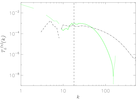
Figure 6: (Color online) Spectral transfer due to the Lorentz force, $T_{L}$ (for $1546^{3}$ DNS) and $T_{L}^{\alpha}$ (for $512^{3}$ $k_{\alpha}=18$ LAMHD) at a time just prior to the peak of dissipation. Positive $T_{L}$ is shown as dash-dotted lines and negative $T_{L}$ as dashed lines. Positive $T_{L}^{\alpha}$ is shown as solid (green online) lines and negative $T_{L}^{\alpha}$ as dotted (green online) lines. LAMHD qualitatively reproduces the transfer of kinetic energy in MHD.

This argument can also be recast in terms of Kelvin’s circulation theorem. For Navier-Stokes, the circulation $\Gamma$ of the velocity $\mathbf{v}$ is conserved in the ideal case for barotropic flows. In ideal MHD, this conservation is broken by the Lorentz force,

$$\frac{d\Gamma}{dt}=\frac{d}{dt}\oint_{\cal C}\mathbf{v}\cdot d\mathbf{r}=\oint_{\cal C}\mathbf{j}\times{\mathbf{b}}\cdot d\mathbf{r},$$ (19)

where ${\cal C}$ is any material curve. As a result, while in ideal Navier-Stokes a material curve ${\cal C}$ defines the boundary of a vorticity tube with fixed strength, in MHD these structures are deformed and their vorticity content changed by the Lorentz force. A similar result follows for LAMHD and LANS,

$$\frac{d\Gamma}{dt}=\frac{d}{dt}\oint_{\cal C}\mathbf{u}\cdot d\mathbf{r}=\oint_{\cal C}\mathbf{j}\times\bar{\mathbf{b}}\cdot d\mathbf{r}\,.$$ (20)

Breaking the conservation of circulation in this way can prevent the formation of a bottleneck. For example, for the fluid case in the Clark$-\alpha$ model (which differs from LANS only in the conservation of $\Gamma$), it was also found that no super-filter-scale bottleneck was present PiGrHoMi+2008 .

III.4 LES Application

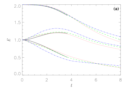
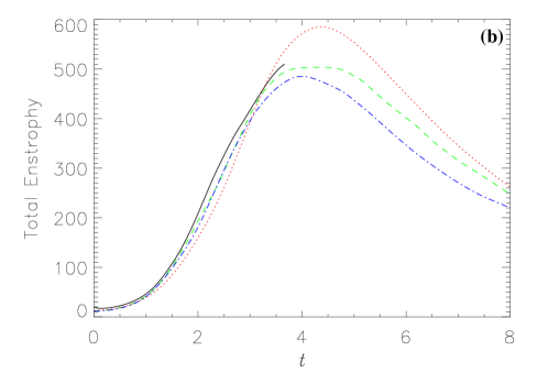
Figure 7: (Color online) Temporal evolution, $\tau_{eddy}\approx 4.5$, for $1536^{3}$ DNS (solid, black), $256^{3}$ $k_{\alpha}=33$ LAMHD (dashed, green online), $256^{3}$ under-resolved “DNS” (dotted, red online), and $384^{3}$ $k_{\alpha}=33$ nonhyperdiffusive-LAMHD (dash-dotted, blue online). (a) Time evolution of the energies: kinetic (lower curves), magnetic (middle curves) and total (upper curves). (b) Time evolution of total enstrophy, $\left<j^{2}+\omega^{2}\right>$ ($\left<j^{2}+\bm{\omega}\cdot\bar{\bm{\omega}}\right>$ for LAMHD and $\left<\mathbf{j}\cdot\bar{\mathbf{j}}+\bm{\omega}\cdot\bar{\bm{\omega}}\right>$ for the nonhyperdiffusive case). Note that LAMHD gives a better agreement to the total dissipation rate up to the maximum time that the high resolution DNS is performed. Also note that the DNS equivalent to the LAMHD run presented here is not feasible on present-day computers at a reasonable cost.

Having now shown that LAMHD does not suffer the same drawbacks with regards to energy spectra as LANS, we may turn our attention to a practical application. The purpose of a SGS model or LES is to make predictions about large Reynolds number flows at a reduced computational expense. From the scaling arguments in Refs. FHT01 ; PGHM+07a , using simulations conducted at $Re\approx 2200$, and assuming a $k^{-1}$ scaling, we can estimate $\alpha=1/33$ for a $256^{3}$ LAMHD-LES “prediction” of our $1536^{3}$ MHD-DNS. Time evolution of the energies and the total enstrophy are shown in Fig. 7 for much later times than reasonably attainable with the MHD DNS with present-day computers. Also shown are results for solving the MHD equations, Eqs. (1) with $\nu=2\cdot 10^{-4}$ and a resolution of $256^{3}$: a so-called “unresolved DNS” and the non-hyperdiffusive modified-LAMHD from the previous section. Before the peak of dissipation, $t\approx 4$, the unresolved DNS gives a poorer prediction of the total dissipation and total energy which is then followed by a significantly larger and somewhat later peak of dissipation, at $t\approx 5$ than the resolved DNS and the LAMHD LES. The non-hyperdiffusive LAMHD is not expected to perform well as a SGS model and it is seen to be clearly under-dissipative. The ratio of magnetic to kinetic dissipation is $\approx 1.5$ for the DNS, $\approx 2.9$ for LAMHD, $\approx 1.1$ for the under-resolved DNS, and $1.4$ for the non-hyperdiffusive model. Together with Fig. 7 (b) these ratios show that LAMHD achieves accurate total dissipation by an excess of magnetic dissipation and a reduction of kinetic dissipation (both at the small scales). This feature has already been depicted in Fig. 15 of Ref. MMP05a . Compensated energy spectra for the peak of dissipation ($t\in[2.7,3.7]$) are shown in Fig. 8. For the under-resolved DNS, we observe the appearance of a tail at large wavenumbers with a $k^{2}$ spectrum as predicted using statistical mechanics arguments for truncated systems in the ideal ($\nu=0$, $\eta=0$) case FrPoLe+1975 . The under-resolved spectra are not significantly different from the resolved DNS, but note that a reliable and convincing determination of spectral indices, beyond visual inspection, does require high resolutions. Comparing now the resolved DNS and the LAMHD run, the quality of the spectra are similar for scales larger than $\alpha$. Recall that differences at the largest scales, stem from the differences in initial conditions as stated in Section III.1, and from time evolution of the flow. Finally, noting that the computer saving here is $6^{3}$ in memory and $6^{4}$ in running time, we conclude that the LAMHD continues to behave satisfactorily, as already shown both in two space dimensions MMP05a ; PGMP05 ; PGHM+06 and in 3D MMP05b , in particular in the context of the dynamo problem of generation of magnetic fields by velocity gradients; thus, LAMHD may prove to be a useful tool in many astrophysical contexts where magnetic fields are dynamically important, such as in the solar and terrestrial environments, or in the interstellar and intergalactic media.

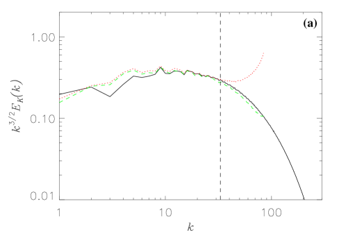
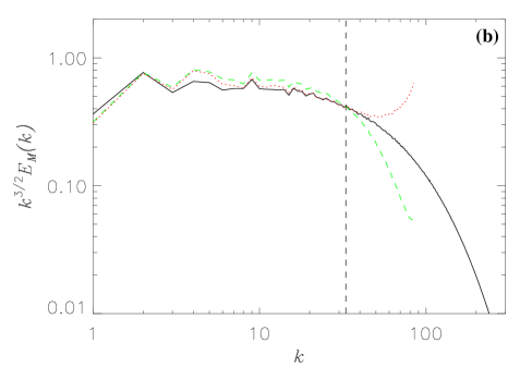
Figure 8: Spectra compensated by $k^{3/2}$ for the kinetic (a) and magnetic (b) energies averaged over $t\in[2.7,3.7]$; labels are as in Fig. 7 and the dashed vertical line indicates $k_{\alpha}=33$. Note the $k^{2}$ tail at high wavenumber that is known to develop for under-resolved runs, a prediction stemming from statistical mechanics.

We also computed a $512^{3}$ LAMHD-LES ($\alpha=1/85$) which retains more of the small scales than the $256^{3}$ LAMHD-LES while still yielding significant computational savings over the $1536^{3}$ DNS. We compare this with the result for $\alpha=1/18$ (chosen not as a LES but to stress the model) in Fig. 9. The structure of sheets observed in MHD dissipative structures is preserved in the LAMHD simulations, although current and vortex sheets become thicker in LAMHD as a result of the filter as $\alpha$ is increased. This is necessary to achieve reduced resolution computations. Note that these sheets are different in nature from the fat ’rigid bodies’ observed in LANS, as the turbulent energy transfer to small scales is not quenched and there is no super-filter-scale bottleneck.

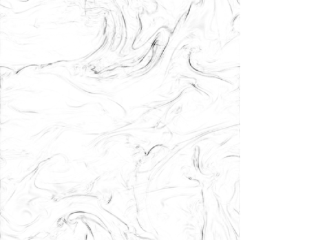
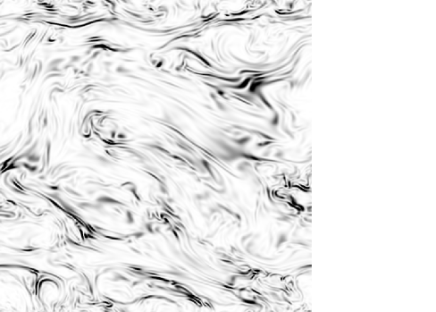
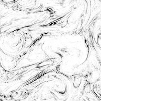
Figure 9: 2D cross sections of square current, $j^{2}$, for $512^{3}$ LAMHD-LES ($\alpha=1/85$) (Upper Left) and model-stress-case ($\alpha=1/18$) (Upper Right). MHD dissipative structures, sheets, are retained which become thicker as $\alpha$ is increased. (Lower Left) $256^{3}$ LAMHD-LES ($\alpha=1/33$) and (Lower Right) $256^{3}$ unresolved DNS. For the unresolved run, current sheets are somewhat smeared out by numerical noise.

IV Discussion

In this paper, we have tested the LAMHD model against high Reynolds number direct numerical simulations (up to Reynolds numbers of $\approx 9200$) and in particular we have focused our attention on the dynamics of small scales near the $\alpha$ cut-off. We find that the small-scale spectrum presents no particular defect; specifically, we find that, unlike in the hydrodynamical case, the Lagrangian-averaged modeling for MHD exhibits, even at large Reynolds numbers, neither a positive-power-law spectrum nor any contamination of the super-filter-scale spectral properties. This difference between LANS and LAMHD is not due to the inclusion of a hyper-diffusive term in LAMHD that stems from the derivation of the model; rather, it stems from fundamental differences between hydrodynamics and MHD. Indeed, neither the (non-consistent) removal of hyperdiffusion from LAMHD nor the examination of scales much smaller than $\alpha$ gave any indication of problems similar to those caused by the zero-flux regions found in computations using LANS. These regions limited the computational gains of using LANS as a LES in hydrodynamics to a factor of only $10$ in computational degrees of freedom or $30$ in computation time. LAMHD is not subject to the same limitations and, as we demonstrated, a gain of a factor of $200$ in the number of degrees of freedom, or a factor of $1300$ in computation time, obtains when comparing to the highest Reynolds number in turbulent MHD available today in a DNS.

There are two obvious candidates to explain the lack of a (super-filter-scale) bottleneck effect in LAMHD: the enhanced (hyper-)diffusion in LAMHD compared with LANS, and physical differences between fluids and magneto-fluids, specifically, spectrally nonlocal transfer via Alfvén waves and its associated breaking of the circulation conservation. The first candidate would eliminate the super-filter-scale bottleneck by removing energy from the system and precluding the formation of a secondary range below the filtering scale $\alpha$ (note that this term becomes of the same order as the ordinary diffusion when $l\sim\alpha$). Simulations of LAMHD performed without the hyper-diffusion term ruled out this scenario, as no super-filter bottleneck was found.

The second candidate is the presence of the Lorentz force in MHD (and LAMHD) which breaks down the circulation conservation and provides the restoring force for Alfvén waves. Both properties were shown to be preserved by LAMHD. In Navier-Stokes, the development of helical filaments could quench local interactions MT92 ; T01 depleting the energy transfer and leading to the viscous bottleneck. However, in MHD, the conservation of the circulation ($d\Gamma/dt=0$ in the absence of dissipation) is broken by the Lorentz force, which modifies Kelvin’s theorem (see Eq. (19)). The forcing term is associated with the Alfvén waves, and represents the removal of circulation (and of kinetic energy) that is transfered to the magnetic field. Note that in Fourier space, the term scales as $kE_{M}(k)$ and is dominant compared to the dissipation in the inertial range. This term precludes the formation of rigid bodies, giving as a result a larger net flux towards smaller scales and a resulting larger dissipation in MHD/LAMHD. This is illustrated in Fig. 4. This sink of circulation may also be the cause of the lack of a viscous-scale bottleneck in MHD. In LANS it was shown PGHM+07a ; PiGrHoMi+2008 that conservation of the circulation (except for viscosity) leads to the formation of rigid bodies that fill a substantial volume of the fluid, and that in turn substantially decrease the energy flux to small scales, reduce dissipation, and create the super-filter scale bottleneck. In LAMHD, the destruction of sub-filter-scale rigid bodies by large scale magnetic field and shear results as the presence of a magnetic field permits the development of long-range interactions in spectral space MAP05 ; AMP05a ; Al2007a . This can also explain why $\alpha-$models for other non-local equations, or for problems that do not preserve the circulation provide good SGS models. As an example, the use of LANS in primitive equations ocean modeling gives satisfactory results, e.g. in its reproducing the Antarctic circumpolar current baroclinic instability that can be seen only at substantially higher resolutions when using direct numerical simulations HeHoPe+2008 .

Energy is dissipated in MHD flows through two different processes. Viscosity is responsible for the dissipation of mechanical energy, while Ohmic losses are responsible for dissipation of magnetic energy. Mechanical and magnetic energy are not conserved separately, but rather coupled as illustrated by the existence of Alfvén waves, which correspond to oscillations of the magnetofluid with the velocity field parallel or anti-parallel to the magnetic field, and associated to the interchange of magnetic and kinetic energy. In MHD, it is believed that most of the total energy in the flow is finally dissipated (mediated by this interchange) through Ohmic losses, in a process that involves reconnection of magnetic field lines. This is supported by several simulations of MHD turbulence HaBrDo2003 ; Mi2007a and is consistent with phenomenology. While in hydrodynamics small scales are permeated by a myriad of vortex filaments, in MHD the dominant dissipative structures are current sheets, where strong gradients of the magnetic field and their associated strong currents lead to rapid Ohmic dissipation. Sub-grid models attempt to replace the physical processes of small-scale dissipation by processes that mimic the non-linear transfer of energy to smaller scales (where energy is in reality dissipated, but now in scales that are not resolved by the model). In traditional LES, this is done with enhanced turbulent viscosities. Note that the eddy viscosity is not obtained from the linear dissipative term (the term that describes the actual physical process responsible for the dissipation) but from the non-linear terms in the equations (the terms that describe the coupling between fields at different scales). The final goal is not to capture the dissipation processes, but to be able to preserve (with computational gains) the large scale dynamics.

Lagrangian averaged models take a different (although related, see e.g., PGHM+06 ) approach. Besides adding (in some cases, as in the case of MHD) an enhanced viscosity, the non-linear terms are modified at small scales. This modification changes the time-scale of the energy cascade, and as a result changes the scaling law of the energy spectrum $E(k)$ at sub-filter scales. This change leads to changes in the dissipation, as the dissipation is in the original equations proportional to $k^{2}E(k)$. The end result (an enhanced dissipation that is intended to mimic the transfer of energy to smaller scales in the unresolved scales) should be the same as in a traditional LES: gains in computing costs preserving as much information of the large scale flow as possible. As in the case of LES, the actual dissipation process is not as important as the fact that large-scale dynamics should be reproduced with minimal contamination by the sub-grid model. We believe the results presented here (and in earlier work MMP05a ; MMP05b ; PGMP05 ; PGHM+06 ; Mi2006a ) show this is the case, and allow the use of the LAMHD equations as a subgrid model of MHD turbulence. However, considering the differences observed between LANS and LAMHD, we discuss the dissipation processes in LAMHD. Two mechanisms for dissipation can be identified in LAMHD: dissipation of mechanical energy through the viscosity, and dissipation of magnetic energy through (enhanced) Ohmic losses. From the equations, the total variation of energy goes as MMP05a : $dE/dt=-\nu\left<\bm{\omega}\cdot\bar{\bm{\omega}}\right>-\eta\left<j^{2}\right>$ and as a result the mechanical energy dissipation scales as $k^{2}E_{V}(k)$ while the magnetic energy dissipation scales as $(1+\alpha^{2}k^{2})k^{2}E_{M}(k)$. The extra $k^{2}$ factor in the latter gives more dissipation than in the LANS case. This excess of magnetic dissipation in LAMHD mimics, as previously mentioned, the dominant contribution to dissipation by Ohmic losses in MHD. This hyperdiffusion is required in the sub-filter scales to accurately model the total energy dissipated at the unresolved scales. This was demonstrated by our experiments with a modified LAMHD, where we (non-consistently) removed the hyperdiffusive term and found the resulting model to fail as a LES.

Yet another way to understand the differences between LANS (for incompressible isotropic and homogeneous flows) and LAMHD is to consider the derivation of these models H02a using the generalized Lagrangian-mean (GLM) formalism AM78 . This form of Lagrangian averaging describes wave, mean-flow interactions. For the case of weak turbulence, where the nonlinear transfer is dominated by waves, GLM requires in principle no closure. As a result, GLM gives an exact closed theory for the evolution of the wave activity. On the other hand, when there are no waves (as in incompressible Navier-Stokes) or when eddies dominate the transfer, a closure is required. One possible closure assumes that fast fluctuations are just advected by the mean flow (basically, Taylor’s frozen-in hypothesis for the small scale turbulent fluctuations) and leads to the several ”$\alpha$-models” that include LANS and LAMHD. In this context, it is not surprising for subgrid models based on GLM to perform better in the presence of Alfvén waves (for LAMHD) or Rossby and gravity waves (for the Lagrangian-averaged primitive equations HeHoPe+2008 ). The more relevant the waves are to the dynamics, and to the non-linear coupling of modes in the system, the less relevant is the hypothesis behind the closure. Furthermore, the $\alpha$-model equations can then be expected to be a better approximation to the problem at hand, that is, to be closer to an exact closure of the original system of equations.

In the fluid case, the application of the “Taylor” closure that smaller-than-$\alpha$ scale fluctuations are swept along by the large-scale flow results in the fluctuations having greatly reduced interactions. This allows for a reduction in computational expense and leads to the super-filter-scale bottleneck by quenching spectrally non-local interactions. In the LAMHD case, the small-scale $\mathbf{z}^{+}$ ($\mathbf{z}^{-}$) fluctuations are swept along by the large-scale $\bar{\mathbf{z}}^{-}$ ($\bar{\mathbf{z}}^{+}$) flow. Small-scale fluctuations advected by two different fields may now collide and nonlinearly interact. The second part of the model is the preferential hyperdiffusion of Alfvén waves with wavelengths shorter than $\alpha$. This damps rather than quenches nonlinear interactions among the small scales. This more gentle suppression of the transfer of energy to smaller scales reduces the numerical resolution requirements without forming a bottleneck.

It was noted in MMP05b when assessing the properties of LAMHD in the dynamo context that the overall temporal evolution was satisfactory, e.g. with a correct growth rate, although the growth of the magnetic seed field started slightly earlier in the LAMHD run than in the DNS. One can speculate as to whether this delay is linked to the super-bottleneck effect of LANS (which prevails when the magnetic field is negligible compared to the velocity, the two modeling approaches, LAMHD and LANS, being dynamically consistent). This point is left for future work; one could determine as well at what ratio of magnetic to kinetic energy the overshooting of spectra in LANS disappears for LAMHD.

Also deserving of a separate study is to investigate the behavior of LAMHD when anisotropies that appear at small scales MiPo2007a are present; this would be essential when a uniform magnetic field is imposed to the overall flow. The evaluation of the behavior of the model when computing spectra in the perpendicular and parallel directions (with respect to a quasi-uniform magnetic field, computed by locally averaging the field in a sphere of radius comparable to the integral scale) remains to be done but is somewhat time consuming. An analysis of the structures that develop in the highly turbulent LAMHD flow studied in the preceding section is also left for future work; of particular interest is the occurrence of Kelvin-Helmholtz like roll-up of current sheets as observed at high resolution MiPo2007a ; however, the choice of the parameter $\alpha$ in the present paper was made on the basis of questioning the existence or lack thereof of a rigid-body high-wavenumber $k^{+1}$ spectrum and, thus, was not optimized for the study of the inertial range properties of the flow for which a much smaller value of the length $\alpha$ could be used.

Finally, how far resolution can be reduced when using LAMHD as a LES for various statistics of interest will also require further detailed study. The present study shows that, to reproduce the super-filter-scale energy spectrum in three dimensions, gains by a factor of 1300 in computing time can be achieved. The need to reproduce higher order statistics can decrease these gains. As an example, in two-dimensional MHD, it was shown that gains when using LAMHD as a subgrid model depend for high order moments on the order that one wants to see to be accurately reproduced PGHM+06 .

- (1) C. Meneveau and J. Katz. Scale-Invariance and Turbulence Models for Large-Eddy Simulation. Annual Review of Fluid Mechanics, 32:1–32, 2000.
- (2) A. Pouquet, U. Frisch, and J. Leorat. Strong MHD helical turbulence and the nonlinear dynamo effect. Journal of Fluid Mechanics, 77:321–354, 1976.
- (3) A. Yoshizawa. Subgrid modeling for magnetohydrodynamic turbulent shear flows. Physics of Fluids, 30:1089–1095, 1987.
- (4) J.-P. Chollet and M. Lesieur. Parameterization of Small Scales of Three-Dimensional Isotropic Turbulence Utilizing Spectral Closures. Journal of Atmospheric Sciences, 38:2747–2757, 1981.
- (5) J. Baerenzung, H. Politano, Y. Ponty, and A. Pouquet. Spectral modeling of magnetohydrodynamic turbulent flows. Phys. Rev. E, 78(2):026310–+, August 2008.
- (6) A. Alexakis, P. D. Mininni, and A. Pouquet. Shell-to-shell energy transfer in magnetohydrodynamics. I. Steady state turbulence. Phys. Rev. E, 72(4):046301–+, 2005.
- (7) P. Mininni, A. Alexakis, and A. Pouquet. Shell-to-shell energy transfer in magnetohydrodynamics. II. Kinematic dynamo. Phys. Rev. E, 72(4):046302–+, 2005.
- (8) Y. Zhou, O. Schilling, and S. Ghosh. Subgrid scale and backscatter model for magnetohydrodynamic turbulence based on closure theory: Theoretical formulation. Phys. Rev. E, 66(2):026309–+, 2002.
- (9) S. Galtier, S. V. Nazarenko, A. C. Newell, and A. Pouquet. A weak turbulence theory for incompressible magnetohydrodynamics. Journal of Plasma Physics, 63:447–488, 2000.
- (10) P. Goldreich and S. Sridhar. Toward a theory of interstellar turbulence. 2: Strong alfvenic turbulence. ApJ, 438:763–775, 1995.
- (11) P. S. Iroshnikov. Turbulence of a Conducting Fluid in a Strong Magnetic Field. Soviet Astronomy, 7:566–+, 1964.
- (12) R. H. Kraichnan. Inertial-range spectrum of hydromagnetic turbulence. Physics of Fluids, 8:1385–1387, 1965.
- (13) J. Mason, F. Cattaneo, and S. Boldyrev. Numerical measurements of the spectrum in magnetohydrodynamic turbulence. Phys. Rev. E, 77(3):036403–+, 2008.
- (14) P. D. Mininni and A. Pouquet. Energy Spectra Stemming from Interactions of Alfvén Waves and Turbulent Eddies. Physical Review Letters, 99(25):254502–+, 2007.
- (15) Annick Pouquet, Pablo Mininni, David Montgomery, and Alexandros Alexakis. Dynamics of the Small Scales in Magnetohydrodynamic Turbulence . In Yukio Kaneda, editor, Proceedings of the IUTAM Symposium on Computational Physics and New Perspectives in Turbulence, Nagoya University, Nagoya, Japan, September, 11-14, 2006, volume 4, pages 305–312. Springer-Verlag, 2008.
- (16) O. Agullo, W.-C. Müller, B. Knaepen, and D. Carati. Large eddy simulation of decaying magnetohydrodynamic turbulence with dynamic subgrid-modeling. Physics of Plasmas, 8:3502–3505, 2001.
- (17) M. L. Theobald, P. A. Fox, and S. Sofia. A subgrid-scale resistivity for magnetohydrodynamics. Physics of Plasmas, 1:3016–3032, 1994.
- (18) N. E. L. Haugen and A. Brandenburg. Hydrodynamic and hydromagnetic energy spectra from large eddy simulations. Physics of Fluids, 18:5106–+, 2006.
- (19) W.-C. Müller and D. Carati. Dynamic gradient-diffusion subgrid models for incompressible magnetohydrodynamic turbulence. Physics of Plasmas, 9:824–834, 2002.
- (20) D. W. Longcope and R. N. Sudan. Renormalization group analysis of reduced magnetohydrodynamics with application to subgrid modeling. Physics of Fluids B, 3:1945–1962, 1991.
- (21) B. Knaepen and P. Moin. Large-eddy simulation of conductive flows at low magnetic Reynolds number. Physics of Fluids, 16:1255–+, 2004.
- (22) Y. Ponty, P. D. Mininni, D. C. Montgomery, J.-F. Pinton, H. Politano, and A. Pouquet. Numerical Study of Dynamo Action at Low Magnetic Prandtl Numbers. Physical Review Letters, 94(16):164502–+, 2005.
- (23) Y. Ponty, H. Politano, and J.-F. Pinton. Simulation of Induction at Low Magnetic Prandtl Number. Physical Review Letters, 92(14):144503–+, 2004.
- (24) D. D. Holm. Averaged Lagrangians and the mean effects of fluctuations in ideal fluid dynamics. Physica D Nonlinear Phenomena, 170:253–286, 2002.
- (25) D. D. Holm. Lagrangian averages, averaged Lagrangians, and the mean effects of fluctuations in fluid dynamics. Chaos, 12:518–530, 2002.
- (26) D. C. Montgomery and A. Pouquet. An alternative interpretation for the Holm “alpha model”. Physics of Fluids, 14(9):3365–3366, 2002.
- (27) P. D. Mininni, D. C. Montgomery, and A. G. Pouquet. A numerical study of the alpha model for two-dimensional magnetohydrodynamic turbulent flows. Physics of Fluids, 17:5112–+, 2005.
- (28) J. Pietarila Graham, P. D. Mininni, and A. Pouquet. Cancellation exponent and multifractal structure in two-dimensional magnetohydrodynamics: Direct numerical simulations and Lagrangian averaged modeling. Phys. Rev. E, 72(4):045301(R)–+, 2005.
- (29) J. Pietarila Graham, D. D. Holm, P. Mininni, and A. Pouquet. Inertial range scaling, Kármán-Howarth theorem, and intermittency for forced and decaying Lagrangian averaged magnetohydrodynamic equations in two dimensions. Physics of Fluids, 18:045106, 2006.
- (30) P. D. Mininni, D. C. Montgomery, and A. Pouquet. Numerical solutions of the three-dimensional magnetohydrodynamic model. Phys. Rev. E, 71(4):046304–+, 2005.
- (31) P. D. Mininni. Turbulent magnetic dynamo excitation at low magnetic Prandtl number. Physics of Plasmas, 13:056502–+, 2006.
- (32) Alexey Cheskidov, Darryl D. Holm, Eric Olson, and Edriss S. Titi. On a Leray model of turbulence. Proceedings of the Royal Society of London, A461:629–649, 2005.
- (33) J. Pietarila Graham, D. Holm, P. Mininni, and A. Pouquet. Highly turbulent solutions of the Lagrangian-averaged Navier-Stokes alpha model and their large-eddy-simulation potential. Phys. Rev. E, 76:056310–+, 2007.
- (34) P.D. Mininni, A. Pouquet, and P. Sullivan. Two examples from geophysical and astrophysical turbulence on modeling disparate scale interactions. In Roger Temam and Joe Tribbia, editors, Summer school on mathematics in geophysics. Springer-Verlag, 2008. to appear.
- (35) D. O. Gómez, P. D. Mininni, and P. Dmitruk. MHD simulations and astrophysical applications. Advances in Space Research, 35:899–907, 2005.
- (36) D. O. Gómez, P. D. Mininni, and P. Dmitruk. Parallel Simulations in Turbulent MHD. Physica Scripta Volume T, 116:123–127, 2005.
- (37) W. H. Matthaeus, A. Pouquet, P. D. Mininni, P. Dmitruk, and B. Breech. Rapid Alignment of Velocity and Magnetic Field in Magnetohydrodynamic Turbulence. Physical Review Letters, 100(8):085003–+, 2008.
- (38) P. D. Mininni, A. G. Pouquet, and D. C. Montgomery. Small-Scale Structures in Three-Dimensional Magnetohydrodynamic Turbulence. Physical Review Letters, 97(24):244503–+, 2006.
- (39) C. Foias, D. D. Holm, and E. S. Titi. The Navier-Stokes-alpha model of fluid turbulence. Physica D Nonlinear Phenomena, 152-153:505–519, May 2001.
- (40) E. Lunasin, S. Kurien, M. Taylor, and E. Titi. A study of the Navier-Stokes-alpha model for two-dimensional turbulence. ArXiv Physics e-prints, 2007.
- (41) Hélène Politano and Annick Pouquet. Dynamical length scales for turbulent magnetized flows. Geophysical Research Letters, 25(3):273–276, 1998.
- (42) R. H. Kraichnan. Inertial Ranges in Two-Dimensional Turbulence. Physics of Fluids, 10:1417–1423, 1967.
- (43) C. Cao, D. D. Holm, and E. S. Titi. On the Clark model of turbulence: global regularity and long-time dynamics. Journal of Turbulence, 6:19–+, 2005.
- (44) P. Dmitruk, D. O. Gómez, and W. H. Matthaeus. Energy spectrum of turbulent fluctuations in boundary driven reduced magnetohydrodynamics. Physics of Plasmas, 10:3584–3591, 2003.
- (45) A. Alexakis. Nonlocal Phenomenology for Anisotropic Magnetohydrodynamic Turbulence. ApJ, 667:L93–L96, 2007.
- (46) J. R. Herring, D. Schertzer, M. Lesieur, G. R. Newman, J. P. Chollet, and M. Larcheveque. A comparative assessment of spectral closures as applied to passive scalar diffusion. Journal of Fluid Mechanics, 124:411–437, 1982.
- (47) D. Lohse and A. Müller-Groeling. Bottleneck Effects in Turbulence: Scaling Phenomena in r versus p Space. Physical Review Letters, 74:1747–1750, 1995.
- (48) D. O. Martínez, S. Chen, G. D. Doolen, R. H. Kraichnan, L.-P. Wang, and Y. Zhou. Energy spectrum in the dissipation range of fluid turbulence. Journal of Plasma Physics, 57:195–201, 1997.
- (49) P. D. Mininni, A. Alexakis, and A. Pouquet. Large-scale flow effects, energy transfer, and self-similarity on turbulence. Phys. Rev. E, 74(1):016303–+, 2006.
- (50) H. K. Moffatt and A. Tsinober. Helicity in laminar and turbulent flow. Annual Review of Fluid Mechanics, 24:281–312, 1992.
- (51) Arkady Tsinober. An Informal Introduction to Turbulence. Kluwer Academic Publishers, Dordrecht, 2001.
- (52) S. Chen, D. D. Holm, L. G. Margolin, and R. Zhang. Direct numerical simulations of the Navier-Stokes alpha model. Physica D Nonlinear Phenomena, 133:66–83, 1999.
- (53) J. Pietarila Graham, D. D. Holm, P. D. Mininni, and A. Pouquet. Three regularization models of the Navier-Stokes equations. Physics of Fluids, 20(3):035107–+, 2008.
- (54) U. Frisch, A. Pouquet, J. Léorat, and A. Mazure. Possibility of an inverse cascade of magnetic helicity in magnetohydrodynamic turbulence. Journal of Fluid Mechanics, 68:769–778, 1975.
- (55) M. W. Hecht, D. D. Holm, M. R. Petersen, and B. A. Wingate. Implementation of the LANS- turbulence model in a primitive equation ocean model. Journal of Computational Physics, 227:5691–5716, 2008.
- (56) N. E. L. Haugen, A. Brandenburg, and W. Dobler. Is Nonhelical Hydromagnetic Turbulence Peaked at Small Scales? ApJ, 597:L141–L144, 2003.
- (57) P. D. Mininni. Inverse cascades and effect at a low magnetic Prandtl number. Phys. Rev. E, 76(2):026316–+, 2007.
- (58) D. G. Andrews and M. E. McIntyre. An exact theory of nonlinear waves on a Lagrangian-mean flow. J. Fluid Mech., 89:609–646, 1978.