Extraction of Resonances from Meson-Nucleon Reactions111Notice: Authored by Jefferson Science Associates, LLC under U.S. DOE Contract No. DE-AC05-06OR23177. The U.S. Government retains a non-exclusive, paid-up, irrevocable, world-wide license to publish or reproduce this manuscript for U.S. Government purposes.
Abstract
We present a pedagogical study of the commonly employed Speed-Plot (SP) and Time-delay (TD) methods for extracting the resonance parameters from the data of two particle coupled-channels reactions. Within several exactly solvable models, it is found that these two methods find poles on different Riemann sheets and are not always valid. We then develop an analytic continuation method for extracting nucleon resonances within a dynamical coupled-channel formulation of and reactions. The main focus of this paper is on resolving the complications due to the coupling with the unstable channels which decay into states. By using the results from the considered exactly solvable models, explicit numerical procedures are presented and verified. As a first application of the developed analytic continuation method, we present the nucleon resonances in some partial waves extracted within a recently developed coupled-channels model of reactions. The results from this realistic model, which includes , , , , and channels, also show that the simple pole parametrization of the resonant propagator using the poles extracted from SP and TD methods works poorly.
pacs:
13.75.Gx, 13.60.Le, 14.20.GkI Introduction
The excited baryon and meson states couple strongly with the continuum states. Thus they are identified with the resonance states in hadron reactions. The spectra and decay widths of the hadron resonances reveal the role of the confinement and chiral symmetry of QCD in the non-perturbative region. Therefore, the extraction of the basic resonance parameters from reaction data is one of the important tasks in hadron physics. Ideally, it should involve the following steps:
-
1.
Perform complete measurements of all independent observables of the reactions considered. For example, for pseudo-scalar meson photoproduction reactions one needs to measure 8 observablestabakin : differential cross sections, three single polarizations , and , and four double polarizations , , , and .
-
2.
Extract the partial-wave amplitudes (PWA) from the data. Here we need to solve a non-trivial practical problem since all observables are bi-linear combinations of PWA; i.e. .
-
3.
Extract the resonance parameters from the extracted PWA. Here the often employed methods are based on the Breit-Wigner formfeshbach , Speed-Plot method of Hoehlerhoehler92 ; hoehler93 , and Time-Delay method of Wignereisenbud ; wigner55 . A more sophisticated and rigorous method is to use the dispersion relations, K-matrix, and dynamical model to analytically continue the PWA to the complex energy plane on which the resonance poles and residues are determined. Extensive works based on these three models are reviewed in Ref.burkertlee .
In reality, we do not have complete measurements for practically all meson-nucleon reactions. Even if the measurements are complete, the step 2 requires some model assumptions to solve the inverse bi-linear problem in extracting PWA. This model dependence must be taken into account in interpreting the extracted resonance parameters.
In this work, we focus on the step 3 in conjunction with the recent efforts in extracting the nucleon resonances from very extensive and high quality data of meson production reactions, as reviewed in Ref.burkertlee . The nucleon resonances listed by the Particle Data Grouppdg are mainly from the analysis of scattering and pion photoproduction reactions. The Speed-Plot and Time-Delay methods are most often used in these analyses since they only require the PWA determined in the step 2. The purpose of this work is to examine the extent to which these two methods are valid and to develop an analytic continuation method within a recently developed dynamical modelmsl of meson production reactions in the nucleon resonance region.
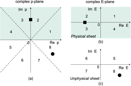
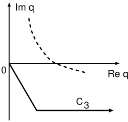
It is useful to first briefly recall how the resonances are defined in textbooks. By analytic continuation, the scattering T-matrix can be defined on the complex energy plane. Its analytical structure is well studiednewton1 ; newton ; peierls59 ; couteur60 ; kato65 for the non-relativistic two-body scattering. For the single-channel case, the scattering T-matrix is a single-valued function of momentum on the complex momentum p-plane, but is a double-valued function of energy on the complex energy E-plane because of the quadratic relation . Therefore the complex E-plane is composed of two Riemann sheets. The physical () sheet is defined by specifying the range of phase , and the un-physical () sheet by . As illustrated in Fig. 1, the shaded area with of the upper part of Fig. 1(a) corresponds to the physical -sheet shown in Fig. 1(b). Similarly, the unphysical -sheet shown in Fig. 1(c) corresponds to the area in the lower part of Fig. 1(a). On the physical sheet, the only possible singularities are on the real E-axis : the bound state poles (solid square in Fig. 1(b)) below the threshold energy and the unitarity cut from to infinity. On the unphysical sheet, a pole (solid circle in Fig. 1(c)) on the lower half plane and corresponds to a resonance. From unitarity and analyticity of S-matrix, each resonance pole has an accompanied pole, called conjugate pole, which exists on the upper half of the un-physical sheet. A resonance pole is due to the mechanism : an unstable system is formed and decay subsequently during the collision. The mathematical details of this interpretation can be found in textbooks, such as in chapter 8 of Goldberger and Watsongw .
For multi-channel case, the analytic structure of the scattering T-matrix becomes more complex newton ; peierls59 ; couteur60 ; kato65 . We postpone the discussion on this until section III where a two-channel Breit-Wigner form of scattering amplitude will be used to give a pedagogical explanation.
The essential point of the Time-Delay and Speed-Plot methods is that the resonance poles discussed above can be determined from the partial-wave amplitudes defined on the physical real energies. The concept of time delay was originally introduced by Eisenbudeisenbud and discussed by Wignerwigner55 , Dalitz and Moorehousedalitz70 , and Nussenzveignussen72 . It is defined as the difference between the time in which a wave packet passes through an interaction region and the time spent by a free wave packet passing though the same distance. It was generalized to the time delay matrix in multi-channel problems and discussed further in terms of a lifetime matrix by Smith smith60 . Kelkar et al.kelkar03b ; kelkar04 applied this multi-channel formulation to develop a practical Time-Delay method to extract hadron resonances.
The Speed-Plot method was developed by Hoehlerhoehler92 ; hoehler93 to extract the nucleon resonances from the partial-wave amplitudes. It is also based on the concept of time delay, but he identified resonances by ”speed” which is the absolute value of the energy derivative of the scattering amplitude. The speed is always positive by its definition while the time delay can be negative and becomes ”time advance” kelkar03a .
It is generally assumed that both the Speed-Plot and Time-Delay methods give approximate positions of the resonance poles which are rigorously defined by the analytic continuation of scattering amplitudes. However their validity is not clear at all. Moreover it is not clear which Riemann sheet the pole positions extracted from using these methods belong to. In this paper we analyze several exactly solvable models to clarify these questions. In particular, we find that these two methods give poles on different Riemann sheets.
We then develop an analytic continuation method for extracting the resonance parameters within a recently developed Hamiltonian formulationmsl of meson-nucleon reactions. We first establish the method by using several exactly solvable models. The main task here is to handle the singularities associated with the unstable particle channels such as , , and . We then apply the method to extract the nucleon resonances in some partial waves of scattering within the dynamical coupled-channels model developed in Ref.jlms . The analytical structure of the resonance propagator is also analyzed within this model.
In section II, we describe the formula for applying the Speed-Plot (SP) and Time-Delay (TD) methods. These two methods are then analyzed and tested in section III by using the commonly used two-channel Breit-Wigner form of S-matrix. In section IV, we develop an analytic continuation method by using several exactly solvable resonance models and further test the SP and TD methods. Section V is devoted to resolve the complications due to couplings with unstable particle channels. In section VI, we present the results from applying the developed analytic continuation method to extract the nucleon resonances in some partial waves within the model of Ref.jlms . A summary is given in section VII.
II Formula for Time-Delay and Speed-Plot Methods
The objective of the Time Delay (TD) and Speed-Plot (SP) methods is to determine the mass and width of a resonance from the S-matrix of reactions. In this section, we will not explain how these two methods were introduced, as briefly discussed in section I. Rather we only give their formula in practical applications.
For the single-channel elastic scattering case, the time delay of the outgoing wave packet with respect to the non-interacting wave packet in a given partial wave is definedwigner55 ; dalitz70 ; nussen72 as
| (1) |
where the S-matrix is related to the phase shift by
| (2) |
Eqs. (1) and (2) lead to a simple expression of time delay
| (3) |
The time-delay (TD) method is to find the resonance mass by finding the maximum of the time delay
| (4) |
As an ideal example, we evaluate the time delay for the S-matrix defined by the well known Breit-Wigner resonance formula
| (5) |
Eq. (1) then leads to
| (6) |
which obviously takes a maximum at and hence is defined as the resonance mass. It also gives the following simple physical interpretation of the width in terms of the time delay of the wave packet passing through the interaction region
| (7) |
Here and in the rest of this paper, the normalization is chosen such that the S-matrix is related to the T-matrix by
| (8) |
We then note that for the S-matrix Eq. (5), the width can also be expressed in terms of T-matrix as
| (9) |
In the analysis of scattering, Hoehlerhoehler92 ; hoehler93 introduced a speed plot (SP) method. The speed is defined as
| (10) |
Using Eqs. (2)-(3), Eq. (10) leads to
| (11) |
Thus the speed is also related to the time delay of the wave packet. The SP method defines the resonance mass by the maximum of the speed
| (12) |
From Eqs. (4), (11), and (12), it is obvious that the speed plot and time delay will give the same resonance mass for the single-channel elastic scattering case.
For the multi-channel reactions with open channels, the S-matrix becomes a matrix . Smithsmith60 introduced a life-time matrix defined by
| (13) |
The above equation can be considered as an extension of Eq. (1) of the single-channel case. The trace of the life-time matrix can be expressed in terms of eigen phases of the S-matrixhazi ; iga04 ; haber
| (14) |
The resonance mass is then obtained by finding
| (15) |
However, the eigen phases can be obtained only when we know all of the S-matrix elements associated with all open channels. In practice, only the elastic scattering amplitude and a few of the inelastic amplitudes can be extracted from the data. Therefore Eqs. (14)-(15) of Smith’s TD method can not be used rigorously in practice.
Here we focus on the TD method used by Kelkar et al.kelkar03a ; kelkar03b ; kelkar04 . They defined the time delay for the channel only by the diagonal component of the S-matrix and its derivative
| (16) |
Obviously, this method is identical to Eq. (1) of the single channel case except that the S-matrix element here is with denoting the inelasticity. Eq. (16) can be considered as an approximation of Eq. (13) by neglecting the inelastic channels in summing the intermediate states. In Refs. kelkar03a ; kelkar03b ; kelkar04 , the resonance mass is determined by the maximum of the time delay
| (17) |
and the width by
| (19) |
The SP method for multi-channel case is simply to define the speed by the diagonal of the T-matrix
| (20) |
and definehoehler92 the width by assuming that the T-matrix element can be parametrized as
| (21) |
Here is an non-resonant amplitude and the resonant amplitude is defined by the resonance mass , the width , and a complex residue . By assuming that the energy dependence of , , and can be neglected at energies near , Eqs. (20) and (21) obviously satisfies Eq. (12) and lead to the following condition
| (22) |
Eqs. (20), (12) and (22) are used in applying the SP method to extract the resonance mass and width from the partial-wave amplitudes. Eq. (21) is not needed in practice, but is an essential assumption of SP method.
III Analysis of Speed-Plot and Time-delay Methods
To examine the SP and TD methods, we consider a commonly used two-channel Breit-Wigner (BW) amplitude which can be derivednewton ; kato65 ; fujii ; fujii75 from the analytical property of the S-matrix. To make the contact with what we will discuss in the rest of this paper, we will indicate here how this amplitude can be derived from a Hamiltonian formulation of meson-baryon reactions, such as that developed in Ref.msl .
It is sufficient to consider the simplest two-channel case with a non-relativistic two-particle Hamiltonian defined by
| (23) |
In the center of mass frame can be written as
| (24) |
where is the mass of -th particle in channel , and is the reduced mass. In each partial-wave, the S-matrix is a matrix and can be written
| (25) |
where is the density of state, and the K-matrix, which is also a matrix, is defined by the following Lippmann-Schwinger equation
| (26) |
Here means taking the principal-value of the integration over the propagator.
We now consider the on-shell matrix element of the S-matrix Eq. (25). If the on-shell momentum is denoted as for channel , we then have
| (27) |
where . The S-matrix element of the elastic scattering is then of the following explicit form
| (28) |
If we assume that at energies near the resonance energy the K-matrix can be approximated as
| (29) |
where is a mass parameter which is a real number, Eq. (28) can then be written as
| (30) |
Here we have defined . If we further assume that is independent of scattering energy, Eq. (30) is the commonly used two-channel Breit-Wigner formulafujii ; fujii75 ; badalyan82 . In the rest of this section, we will follow these earlier works and treat and as energy independent parameters of the model.
Since the scattering T-matrix is related to the S-matrix by
| (31) |
Eq.(30) leads to
| (32) | |||||
From nowon we use the notation for the amplitude .
III.1 Analytic Properties of the S-matrix
Within the two-channels Breit-Wigner model specified above, we will analyze in this subsection the analytic properties of the S-matrix on the complex energy E-plane. This will also allow us to explain clearly some terminologies which are commonly seen but often not explicitly explained in the literatures on resonance extractions.
The on-shell momenta for channel is defined by
| (33) |
where
| (34) |
We can define the threshold variable between two channels by
| (35) |
where
| (36) |
is the threshold energy of the second channel.
The momenta at poles of the S-matrix Eq. (30) can be determined by solving
| (37) |
By using Eqs. (33)-(36), the above equation can be written as
| (38) |
where
| (39) | |||||
| (40) | |||||
| (41) | |||||
| (42) |
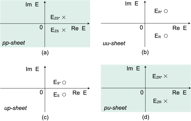
Eq. (38) means that the Breit-Wigner amplitude Eq. (30) has four poles. Each pole is specified by two on-shell momenta with . The analytic properties of the S-matrix Eq. (30) depends on how these poles are located on the complex energy -plane. As we explained in section I, the energy plane for each channel has two Riemann sheets because of the quadratic relation Eq. (33) between the momentum and energy ; namely for . For each channel, the physical () sheet is defined by specifying the range of phase , and the un-physical () sheet by . The correspondence between the momentum -plane and the energy -plane is similar to that illustrated in Fig. 1. For the considered two-channel case, we thus have four energy sheets specified by the signs of and : , , , and , as shown in Fig.2. Thus each of four poles can be on one of these E-sheets.
To be more specific, we now consider the case which is most relevant to our study of nucleon resonances. That is the and case that the poles are all above the thresholds of both channels. From Eq. (37), we immediately notice that if with is one of the solutions, with is also a solution. Therefore the four poles determined by Eq. (38) can be grouped into two pairs. In the following discussions, they are denoted as and . Without losing generality, one can assume that one of the poles is in the range of () and the other in the range of (). If the first pole is in the region where (, ) and (, ) , it is a pole, denoted as , on the -sheet of Fig. 2. This pole is usually called the resonance pole and is closer than other poles on or -sheets to the physical -sheet, as will be explained later. In the Hamiltonian formulation considered in this work and the well developed collision theory, a resonance pole can be mathematically derivedgw from the mechanism that an unstable system is formed and decay subsequently during the collision. The resonance pole has an accompanied pole at which is also on the -sheet as shown in Fig. 2. is called the ’conjugate pole’ of .
The second pole at with and ( and ) may be on the -sheet (-sheet), depending on the parameters and . This pole is called the shadow poleeden64 . A shadow pole on -sheet and its conjugate pole are and in Fig. 2.
We now note that in this simple BW model, the zeros of the S-matrix Eq. (30), where , is defined by its numerator
| (43) |
The above equation can be cast into the form of Eq. (37) by simply replacing by . Thus solutions of Eq. (43), called the zeros of S-matrix, can be readily obtained from the solutions and of Eq. (37). They are with and with for . The zero at is on the -sheet, denoted as and in Fig. 2. Similarly, the zero at is on the -sheet, shown as together with its conjugate in Fig. 2. Note that Fig. 2 is for the case that the parameters and are chosen such that the shadow poles and its conjugate are on the -sheet. For other possible and , the pole positions could be different from what are shown in Fig. 2, but their close relations, as discussed above, are the same.
From the above analysis, it is clear that the poles and zeros of the S-matrix are closely related. Their locations on the 4 Riemann sheets can be conveniently displayed on one complex plane by introducing a variable newton-book
| (44) | |||||
| (45) |
Hence each point in the plane corresponds to a set of . In Fig. 3, the resonance position and shadow poles and their conjugate poles and zeros of S-matrix are shown on t-plane. The physical S-matrix at real energies, which determine the observables, are on the bold lines. The zero energy and the threshold of the second channel correspond to and , respectively. One can see that the resonance pole is closer than the shadow pole to the bold lines (S-matrix) and hence can have the largest effect on the observables. Consequently, most of the rapid energy dependence of observables are attributed to the resonance poles, not the shadow poles or the other poles shown in Fig.3. On the other hand, the zero of the S-matrix is also close to the bold lines. As seen in the derivations given above, this zero is closely related to shadow pole . Thus the shadow poles can also be related to the observables. Of course, which pole is most important in determining the rapid energy dependence of observables also depends on the residues of the T-matrix at the pole positions.

In the next subsection, we will use a further simplified BW form to explain more clearly the close relations between the poles and zeros of the S-matrix. In particular we will see explicitly that the shadow pole in Fig. 2, which is not on the same Riemann sheet as , can be located by the zeros of the S-matrix. More importantly, we will also see how the SP and TD methods work both analytically and numerically.
III.2 Positions of poles
For simplicity, we assume that the threshold energies of the two channels are the same and hence and . Therefore we have simple relations between energy and momenta : and . As discussed in the previous subsection, the four Riemann sheets are classified by the sign of the imaginary part of the momentum; namely, physical (unphysical) sheet is assigned by . With the simplification , we obviously have on the and -sheets, and on and -sheets.
Let us start with the case of for the -sheet or -sheet. The S-matrix element Eq. (30) of the first channel can be written as
| (46) |
It can be cast into the following more transparent form
| (47) |
with
| (48) | |||||
| (49) |
where
| (50) |
Remembering that we consider and . To make use of Fig.2 in the following discussion, we consider the case that and hence and both and defined in Eqs. (48)-(49) are associated with the unphysical -sheet. For the case of , is associated with the physical -sheet and the following presentation can be easily modified to account for this case.
Clearly, Eq. (47) means that the S-matrix has a pole at on the -sheet with a resonance energy
| (51) |
Its conjugate pole is at . The positions of and are shown in the upper right side of Fig.2. Eq. (47) also indicates that the zero of S-matrix is at which is on the -sheet because of . The energy of this zero of S-matrix is
| (52) |
Its conjugate is at . The positions of and are on the -sheet, as shown in the upper left side of Fig.2.
We next consider the case that the poles and zeros of the S-matrix are on the or -sheets. The S-matrix Eq. (30) for this case then takes the following form
| (53) |
By comparing Eq. (46) and Eq. (53) and using the variables and defined by Eqs. (48) and (49), Eq. (53) can be written as
| (54) |
The above equation indicates that for the considered , the S-matrix has a shadow pole at on the -sheet. Thus its position is identical to of the zero of the S-matrix on the -sheet; namely
| (55) | |||||
This means that the shadow pole on the -sheet can be found from searching for the zero of S-matrix on the -sheet.
Eq. (54) also gives a zero of S-matrix at on -plane because . Its energy is also identical to defined above
| (56) | |||||
The positions of and and their conjugates and are also in the lower parts of Fig.2.
From the above analysis for the case, we see that the energies of the resonance poles may be obtained by studying the poles of the S-matrix on the -sheet and those of the shadow poles may be obtained from the zeros of the S-matrix on the -sheet. The analysis for the case is similar. Here we only mention that when is changed to , the shadow poles and on the -sheet move to the -sheet and zeros and will be on the -sheet.
Now let us examine how the SP and TD methods can find the poles defined by the above exact expressions of the two-channel BW amplitude. We first recall that in applying the SP and TD methods, the energy and momentum in the S-matrix are restricted on the positive real-axis. For the considered simplified case, we thus have and the -matrix Eq.(32) then becomes
| (57) |
Our task is to examine whether the resonance mass and width found by applying the SP and TD methods on the expression Eq.(57) are close to the real and imaginary parts of the poles defined in the previous subsection.
According to Eqs. (12) and (20), the SP method finds the resonance mass by finding the maximum of the speed through the use of the condition
| (58) |
With the T-matrix Eq.(57), Eq. (58) leads to the following equation
| (59) |
This equation can be written in the dimension-less form as
| (60) |
with . With some inspections, one can see that Eq. (60) has real and positive solutions only in the region. Two of the three solutions are the maximum and minimum points of the speed, and the third one is less than 0. The SP method defines the maximum point of the speed as the resonance mass. We find that this solution can be expanded as
| (61) |
Clearly, equals to the real part of Eq. (51) if we neglect the second and higher order terms in the expansion in powers of . Therefore the SP method is accurate only under the condition that . Moreover, it is clear from the above equation that speed has no stationary point for and therefore the SP method will fail to find the pole even if there is a pole within the model.
We next turn to discussing the width obtained by the SP method. It is evaluated by using Eq. (9). We find that it can also be expanded as
| (62) |
Here again, if we neglect higher order terms of , the SP method can give the imaginary part of of the exact expression Eq. (51). As we have seen in Fig.2, the two-channel BW S-matrix has two pairs of poles on the -sheet and the -sheet. However the SP method can only find the pole on the -sheet.
From the above analysis, it is clear that the accuracy of SP method is controlled by . We examine this by using an example with , and , and . In Fig.4 the solid curves are the pole positions on the -sheet. They are obtained from evaluating the exact analytical formula Eq. (51) for and varying from to . With the same parameters we then apply the SP method to search for pole from the amplitude Eq. (57) numerically by using Eqs. (9), (10) and (12). The obtained pole positions were the filled squares shown in Fig.4. As expected, the SP method works very well for small . However the pole position from SP starts to deviate from the exact results (solid curves) as increases. There is no filled squares in Fig.4 in the region because the SP can not find a pole in this region. This is not because of the numerical accuracy of our calculation, but is the intrinsic limitation of the SP method as, discussed above.


We now turn to investigating the TD method. We apply Eq. (17) to search for the resonance mass from the amplitude Eq. (57). Since it is not clear how to interpret Kelkar’s prescription Eq. (19), we assume that the S-matrix element is of the following form
| (63) | |||||
| (64) |
Then Eq. (19) leads to an improved expression for the width
| (65) |
where of is for the maximum(minimum) of the TD suggesting the pole on - (-) sheet. We have found that the TD method, defined by Eq. (17) and Eq. (65) can only find the shadow poles on the -sheet which are given by exact expression Eq. (55). The results from using the same parameters specified above are also shown in Fig.4. The dashed curves are from the exact expression Eq. (55) and the solid dots are from applying Eq. (17) and Eq. (65) to search numerically for the poles from Eq. (53). Clearly TD method works very well in finding the shadow poles on -sheet. In the same figure the triangles are from using Kelkar’s prescription Eq. (19). Obviously, our formula Eq. (65) works better. We have also examined TD for . In this case the TD becomes negative and has minimum. We apply Eq. (17) for the minimum of TD and find that TD works also well in finding the pole on -sheet.
IV Analytic continuation of resonance models
With the analysis presented in the previous section, it is clear that the empirical partial-wave amplitudes determined from experimental data can not be blindly used to extract resonance parameters by using SP or TD methods. To make progress, one needs to construct a reaction model to fit the data and then extract the resonance parameters by analytic continuation within the model. In this paper, we focus on a dynamical modelmsl which accounts for the main features of meson production reactions in the nucleon resonance region. Our task in this section is to develop numerical methods for finding the resonance poles from such models which do not have analytical forms of their solutions. We will first consider the simplest one-channel and one-resonance case, then two-channels and one-resonance, and finally two-channels and two-resonances cases. All of these models are exactly solvable such that their poles are known analytically and the developed numerical methods can be tested.
IV.1 One-channel, one-resonance
To be specific, we consider the two-particle reactions defined by the following well known isobar Hamiltonian in the center of mass frame
| (66) |
with
| (67) | |||||
| (68) |
where is the mass parameter of a bare particle which can decay into two particle states through the vertex interaction in , and is the energy of the -th particle. The scattering operator is defined by
| (69) |
which leads to the following Lippmann-Schwinger equation for the scattering amplitudes in each partial-wave
| (70) |
where the integration path will be specified later. The interaction in Eq. (70) is
| (71) |
Eqs. (70)-(71) leads to the following well known solution
| (72) |
with
| (73) |
From the analysis in the previous section, the resonance poles can be found from on the unphysical Riemann sheet defined by with denoting the on-shell momentum
| (74) |
Obviously is also the pole position of the propagator in Eq. (70) or Eq. (73).
The physical scattering amplitude at a positive energy can be obtained from Eq. (70) or Eq. (72) by setting with a positive and choosing the integration contour to be along the real-axis of with . From Eq. (70) it is clear that has a discontinuity on the positive real
| (75) | |||||
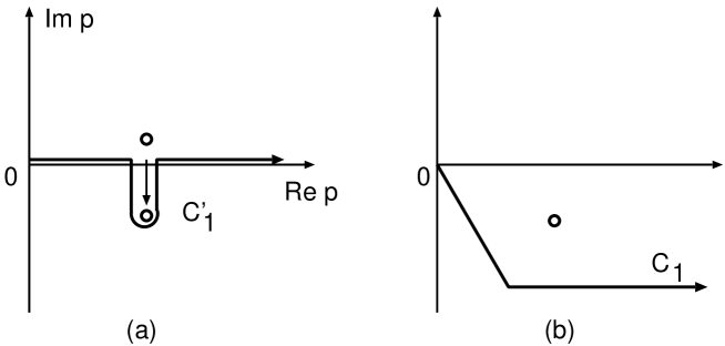
where . Thus the t-matrix has a cut running along the real positive . To find resonance poles, we need to find the solution of Eq. (70) on the un-physical sheet with on which the pole of the propagator moves into the lower p-plane, as shown in (a) of Fig.5. From Eq. (75), it is clear that the solution of Eq. (70), with the contour chosen to be on the real-axis , will encounter the discontinuity and is not the solution on the unphysical sheet where we want to search for the resonance poles. It is well-knownbadalyan82 ; orlov84 ; pearce84 ; pearce89 that this difficulty can be overcame by deforming the integration path to the contour shown in (a) of Fig.5. By this the pole will not cross the cut and the integral is analytically continued from real positive to the lower half of the unphysical E-sheet with . Obviously, the same solution can be obtained by choosing any contour which is below the pole position , such as the contour of (b) of Fig.5.
With the solution of the form of Eq. (72), the numerical procedure of finding resonance poles is to solve
| (76) |
with
| (77) | |||||
| (78) |
for on the unphysical Riemann sheet defined by . To test this numerical procedure, let us consider the case that defined by Eq. (73) can be calculated analytically. Such an analytic form can be obtained by taking the non-relativistic kinematics with and a monopole form for the vertex function
| (79) |
where is a cut-off parameter. The integration in of Eq. (73) can then be done exactly to give the following simple form
| (80) |
where is defined by . If the imaginary part of is positive (negative), it means that we choose the poles on physical (unphysical) sheet. Only the pole with on the unphysical sheet is called resonance, as discussed in the previous section.
The resonance poles on the unphysical sheet () obtained from using Eq. (80) to solve Eq. (76) are the solid curve displayed in Fig.6 using the parameters: , , and cutoff momentum , for a range of coupling constant . We next solve Eqs. (76) and (78) by choosing contour illustrated in Fig.5. The solutions are stable as far as the path is not too close to the pole. The solutions completely agree with the solid curve of the exact solution and hence are not displayed in Fig. 6. Here we also note that Eq. (80) also allows to calculate the poles by using the SP and TD methods. The results for the value of , , , are the solid squares in Fig.6. As expected we confirm the previous findings that both SP and TD work well for the single channel case.

IV.2 Two-channels, one-resonance
The formula for two-channels, one-resonance case can be easily obtained by extending the equations in the previous subsection to include channel label . We thus have
| (81) |
where with denoting the mass of -th particle in channel , and
| (82) |
| (83) |
with
| (84) |
For the physical scattering amplitude at a positive energy E, Eq. (81) is solved by setting with a positive and choosing along the real axis .
With Eq. (83), the poles of the scattering amplitudes are defined by
| (85) |
The poles from solving the above equation can be on one of the four Riemann sheets, , , , and , as explained in section III. The numerical procedure for finding the resonance poles on -sheet is to solve Eq. (85) for with and . The integration path is changed to shown in (b) of Fig.5 to calculate both self-energies and of Eq. (84). Of course the contour for the integration over the momentum for -th channel must be below the pole defined by . Here we note that for finding the poles on -sheet (-sheet), the contour is replaced by only for ().
To test numerical procedures and to further test the SP and TD methods, let us consider again the non-relativistic kinematics with and . This will allow us to find the exact solutions by choosing the monopole form factor
| (86) |
We then have
| (87) |
With Eq. (87), the poles defined by Eq. (85) can be found by solving algebraic equations. For numerical calculations, we consider a case similar to scattering in partial wave: (1)channel-1 is with MeV , MeV, and , (2)channel-2 is with MeV , MeV, and , (3) bare mass . The results are shown in Fig.7. The dash-dotted (solid) curves are the calculated poles on -sheet (-sheet) with the coupling constants for and a range of for . We see that when is 0, which is the single-channel case, the -pole and the -pole are on the same position. They then split as increases.
We next evaluate Eq. (84) for on the -sheet, -sheet or -sheet by appropriately choosing the path , as described above. The poles are found when the calculated and satisfy Eq. (85). We find that the poles obtained by this numerical procedure reproduce accurately the dash-dotted(-sheet), solid(-sheet) and dashed(-sheet) curve in Fig.7 and hence are omitted there. Thus this analytic continuation method can be used in practice to find the resonance poles (i.e. poles on -sheet as defined in section III) for general case that can not be integrated analytically.
We now turn to examining the SP and TD methods. In Fig.7, we show that the SP method (open squares) reproduces the poles (dash-dotted curve) on the -sheet only at . When is larger than 0.015 where the magnitude of continues to increase, the speed has no maximum and the SP method fails to find the pole. This is another example showing that SP method has its limitation. On the other hand, the TD method (solid squares) can reproduce the poles on the -sheet (solid curve) and -sheet (dashed curve) in the considered range of parameters. Here we see that the SP and TD find different poles which have different physical meanings in the Hamiltonian formulation. One can showgw that the poles on -sheet are due to the process that an unstable system is created and then decays during the collision and are called the resonance poles. The physical interpretations of the poles on and -sheets remain to be developed.

It is interesting to point out here that the two-channel Briet-Wigner form analyzed in detail in the previous section can be derived from the two-channels, one-resonance model if the non-relativistic kinematics is used. To see this, we first write the non-relativistic relation between the S-matrix and the T-matrix
| (88) | |||||
| (89) |
where is the on-shell momentum in channel
| (90) |
With the above and the analytic form Eq. (87) for , we can write the elastic scattering amplitude of Eq. (89) as
| (91) |
where and
| (92) |
where means taking the principal-value integration. By using Eq. (88), we then have the elastic part of the S-matrix
| (93) |
If the E-dependence of and are further neglected, Eqs. (91) and (93) are identical to what are usually called the two-channel Breit-Wigner resonant amplitude discussed in the previous section. Thus the conditions under which SP and TD are valid can be related now to the parameters of the vertex function within this two-channels, one-resonance model.
IV.3 Two-channels, two-resonances
For the two-channels, two-resonances case, the scattering amplitude is defined by the same Eq. (81), but with the following driving term
| (94) |
The scattering amplitude is then of the following form
| (95) |
The propagator in Eq. (95) is
| (96) |
with
| (97) |
The poles are defined by
| (98) | |||||
The numerical procedures of finding the resonance poles on the -sheet from Eqs. (97) and (98) are the same as that in the previous two subsections. Namely the path of Eq. (97) is set to be the path shown in Fig.5 in evaluating the integrals for on the -sheet where the on-shell momenta are for channels. To test this, we again choose the non-relativistic kinematics and the monopole form factor like Eq. (86). The self energy then takes the analytic form similar to Eq. (80). The condition Eq. (98) can then be expressed in a analytic form from which the pole positions on the unphysical sheet can be easily obtained.
We only state that the resulting poles on the unphysical sheets are reproduced by the numerical analytic continuation method described above. Instead our focus here is to further test the SP and TD methods for the situation that two resonances are close and could overlap. We again consider and channels and use the following form factor
| (99) |
where denote the -th bare state with mass . The four cut-off parameter and four coupling constants are taken to be: MeV, , , and . One of the bare masses is fixed in the calculations. is defined by
| (100) |
where is varied for examining how the poles move as moves away from the MeV.
The pole positions are searched numerically by using the analytic continuation method described above. There are two poles on the -sheet and the other two on the -sheet. As varies, these two poles will develop two trajectories. They are the crosses connected by the solid curves shown in Fig.8 for -sheet and Fig.9 for the -sheet. According to the findings we made in section III, the poles, , found by the SP (TD) method should be compared with the poles on () sheet of Fig. 8 (9). We now discuss these two comparisons.
We see from Fig. 8 that in the regions near MeV, the positions () of these two poles are far from each other and we find that SP (open squares connected by dashed lines near the point marked 700) works well. When is reduced to MeV where the positions () of two poles move closer, the SP method can find only one pole ( open squares connected by dashed line) near the top end of the trajectory on the right hand side. Apart from the points on the dashed lines, SP method fails to find poles close to the poles on the solid curves which are obtained numerically by the analytic continuation method.
The results for examining TD is shown in Fig.9. We see that TD can find two poles on the -sheet in the considered range of . The results are the open squares connected by dashed lines which are indistinguishable from the crosses connected by solid curves which were obtained by analytic continuation method. But TD obtains another two poles at and , as indicated by the dashed line in the middle of Fig.9. The positions of these two poles are very close to those obtained from SP and they are interpreted as poles on -sheet. As we have discussed in section II, TD is sensitive to both zero and pole of the S-matrix on and -sheets. In this example, width of the poles on -sheet become comparable to the poles on -sheet(zero on physical sheet) and hence TD could find pole on -sheet. The results shown in Fig. 8 and Fig. 9 further indicate the limitation of SP and TD methods.
The results from the above several models have shown that the TD method based on Eq. (16), where the phase of the elastic channel is used instead of the eigen phases discussed in Refs. hazi ; iga04 ; haber , gives both the resonance poles on the -sheet and the zeros(shadow poles). Our findings could provide some information for investigating the differences between Refs.haber andkel2008 . We also want to mention here that an improved SP method using higher order derivatives of the amplitudes was proposed in Ref. ceci2008 . It may be interesting to compare this method with the TD method. While it could be interesting to address the questions concerning these recent developments, they are far from the main focus of this paper and will not be discussed further.


V Analytic continuation of resonance model with unstable particle channels
For meson-baryon reactions, the nucleon resonances can decay into some unstable particle channels such as the , , considered in the model of Ref.msl . Here we discuss the analytic continuation method to find resonance poles within such a reaction model.
It is sufficient to consider the one-channel and one resonance case. The scattering formula is then identical to that presented in subsection IV.A. The only difference is that one of the particles in the open channel can further decay into a two particle state. To be specific, let us consider the channel. Within the same Hamiltonian formulationmsl used in the previous section, the scattering amplitude can then be written as
| (101) |
with
| (102) |
where
| (103) |
To obtain the self energy for complex , the analytic structure of the integrand of Eq. (102) should be examined first. The discontinuity of the propagator in the integrand of Eq. (102) is the cut along the real axis between () which is obtained by solving
| (104) |
For finding the resonance poles on -sheet with , the integration contour of Eq. (102) must be chosen below this cut which is the dashed line in Fig.10. There is also a singularity in the integrand of Eq. (102) at momentum , which satisfies
| (105) |
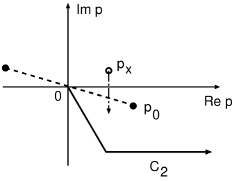
Physically, this singularity corresponds to the two-body scattering state. For with large imaginary part, can be below the cut as also indicated in Fig.10. Therefore the integration contour of momentum must be chosen to be below the cut (dashed line) and the singularity , such as the contour shown in Fig.10.
The singularity position of the propagator in Eq. (103) depends on spectator momentum
| (106) |
Therefore the singularity moves along the dashed curve in Fig.11 when the momentum varies along the path of Fig.10. To analytically continue from positive energy to the un-physical plane with , we need to choose the contour of Eq. (103) which must be below . A possible contour is the solid curve in Fig.11.
To verify the numerical procedures described above, we again consider non-relativistic kinematics and monopole form factor. With the similar analytic form Eq. (80), we have
| (107) |
where
| (108) |
with . With Eq. (107), we can solve Eq. (105) and verify its relation with cut as discussed above and illustrated in Fig.10. Eq. (107) and the chosen monopole form factor also allow us to get
| (109) |
with
| (110) |
Unfortunately, Eq. (109) can not be integrated out analytically for directly checking our numerical procedure for searching resonance poles.
We test our analytic continuation method by the following procedure. We calculate Eq. (109) numerically to find the pole position by solving of the denominator of Eq. (101). With the parameters:
| , |
we find MeV. We then construct an approximate propagator
| (111) |
For the positive E, we find that is in good agreement with the direct calculation of by using Eq. (109). The results are shown in Fig.12. It is clear that the resonance pole found by our analytic continuation method can reproduce what is expected for a resonance propagator for real positive E. In this way our numerical procedure is justified and can be applied to solve Eqs. (101) - (103).

VI Resonance model with non-resonant interactions
With the numerical methods described above, we can proceed to extract the resonance poles within a coupled-channels model which also include non-resonant interactions. In this section, we explain how this can be done for the model developed in Refs.msl ; jlms .
Recalling the formulations presented in Refs.msl ; jlms , the t-matrix considered is of the following form
| (112) |
where can be stable channels and , or unstable channels , and , and denotes a bare resonant state with a mass .
For extracting resonance poles, we now apply the methods presented in previous sections to choose appropriate contours for calculating various integrations on unphysical E-plane with . The non-resonant t-matrix is defined by the following couple-channel equations with the non-resonant potential ,
| (113) |
where the contour is ((b) of Fig.5) for , and (Fig.10) for , and
| (114) |
The self-energies in Eq. (113) are and , , and are defined by the same Eq. (102) with appropriate changes of mass parameters and the choice of contour and shown in Figs. 10 and 11.
The dressed vertex is determined by the bare vertex and the meson-baryon loop,
| (115) |
The resonance propagator in Eq. (112) is
| (116) |
with
| (117) |
In Ref.jlms , the above equations are solved on the real-axis by using the standard method of subtraction. Here we solve the equations by choosing contours indicated above. We first verify that our numerical results obtained here for positive real E agree with that of Ref.jlms . This establish our numerical procedure in this complex five-channel model.
Here we show the results for some of the , , , and partial waves of scattering within the model of Ref.jlms . We search the resonance poles by looking for zeros of the resonant propagator defined by Eq. (116). Our results from using the analytic continuation method are shown in the second column of Table 1. They are compared with those extracted by using SP and TD methods described in the previous sections as well as the values listed by PDG. The Breit-Wigner resonance parameters are also given by PDG, but are not considered here. We see in Table 1 that the SP method fails to find the first resonance pole in the partial wave. We also see that while the real parts of the resonance poles from different approaches are within the ranges of PDG, the extracted imaginary parts can differ by as much as a factor of two or three.
The model of Ref.jlms is currently being improved by also fitting other data of and reactions. For example, some progress has been made to also fit the data of kjlms08 , jlmss08 , and djlss08 . We thus do not include the results for other partial waves in Table 1. Our purpose here is to simply demonstrate how the analytic continuation method works for a realistic model. The full resonance parameters, including the extracted residues and the relations to the Breit-Wigner parameters listed by PDG, extracted from our complete analysis of all will be reported elasewhere.
| Analytic Continuation | Speed PLot | Time Delay | PDG | |||||
|---|---|---|---|---|---|---|---|---|
| Re | Im | Re | Im | Re | Im | Re | Im | |
| S11 | 1540 | -191 | - | - | 1543 | -52 | 1490 1530 | -45 -125 |
| 1642 | -41 | 1644 | -89 | 1645 | -61 | 1640 1670 | -75 -90 | |
| S31 | 1563 | -95 | 1574 | -67 | 1616 | -53 | 1590 1610 | -57 -60 |
| P33 | 1211 | -50 | 1212 | -49 | 1212 | -49 | 1209 1211 | -49 -51 |
| D13 | 1521 | -58 | 1525 | -57 | 1522 | -11 | 1505 1515 | -52 -60 |
| F15 | 1674 | -53 | 1671 | -59 | 1683 | -24 | 1665 1680 | -55 -68 |
We now turn to discussing whether the extracted resonance pole can be used to evaluate the propagator defined by Eq. (116) for the physical positive E. Let us consider the case listed in Table 1. Its propagator can be written as
| (118) | |||||
| (119) |
By using the analytic continuation methods described in the previous sections, the resonance energy MeV is found numerically by solving
| (120) |
We now perform the Laurent expansion of for real around the pole position
| (121) | |||||
The naive works well for a model studied in the previous section. However when the enery dependence of the self energy becomes large, two important modifications should be considered: (1) at the pole, the residue is not one but modified by the field renormalization factor . (2)The second term of the last expression gives a constant term.
With the above expansion Eq. (121), we can introduce three different approximate forms for the propagator
| (122) | |||||
| (123) | |||||
| (124) |
In Fig.13, we compare the above three approximate propagators with the exact result of of Eq. (118). The simple (dashed curves) of Eq. (122) are far from the exact green function (cross) defined by Eq. (118). When the factor is included, we obtain the dashed-dotted curves for . The solid curves are from . We see that the constant term of Eq. (124) mainly affects the imaginary part of the propagator.
Eq. (121) shows that the simple pole approximation , which can be cast into the usual Breit-Wigner form with and , works poorly. We also find that the pole parametrization of the resonant propagator using the poles extracted by the TD and SP methods also work poorly. For the considered case, the pole positions from using these two methods are: and , as given in Table 1. In Fig.14, we compare the exact propagator (cross) of Eq. (118) with the following two propagators
| (125) | |||||
| (126) |
Clearly, phenomenological forms Eqs. (125)-(126) can not account for the complex coupled-channel resonant mechanisms.


VII Summary
In this paper, we have presented a pedagogical study of the commonly used Speed-Plot (SP) and Time-Delay (TD) methods for extracting the resonance parameters from the empirically determined partial-wave amplitudes. Using a two-channel Breit-Wigner form of the S-matrix, we show that the poles extracted by using theses two methods are on different Riemann sheets. The SP method can find resonance poles on the unphysical -sheet, while the TD method can find poles and zeros of S-matrix on or -sheets and therefore its validity is sensitive to the poles on or -sheets. Furthermore, we also show numerically that these two methods can fail to find those poles. Our results support the previous findings that these two methods must be used with cautions in searching for nucleon resonances from the meson-nucleon reaction data in the region where the coupled-channel effects are important.
We then develop an analytic continuation method for extracting the resonance poles within a Hamiltonian formulation of meson-nucleon reactions. The main focus is on resolving the complications due to the coupling with the unstable , , and channels which can decay into states. Explicit numerical procedures are presented and verified within several exactly solvable models. The results from these models are also used to further demonstrate the limitation of the SP and TD methods.
As a first application of the developed analytic continuation method, we present the results from analyzing the , , , and amplitudes of the dynamical coupled-channels model of reactions developed in Ref.jlms . We also analyze the resonance propagators and show that the simple pole parametrization of the resonant propagator using the poles extracted from SP and TD methods works poorly.
With the progress made in this work, we can proceed to extract all nucleon resonance parameters within the model of Ref.jlms . However, this can be done more accurately only when the coupling with the unstable , and channels are better determined by also fitting the two-pion production data. Our progress in this direction will be reported elsewhere.
Acknowledgements.
This work is supported by the Japan Society for the Promotion of Science, Grant-in-Aid for Scientific Research(C) 20540270, and by the U.S. Department of Energy, Office of Nuclear Physics Division, under contract No. DE-AC02-06CH11357, and Contract No. DE-AC05-060R23177 under which Jefferson Science Associates operates Jefferson Lab.References
- (1) Wen-Tai Chiang and Frank Tabakin, Phys. Rev. C 55 (1997) 2054.
- (2) For example, see the text book Theoretical Nuclear Physics : Nuclear Reactions by Herman Feshbach, John Wiley Sons, Inc (1992).
- (3) G. Hoehler and A. Schulte, N Newsletter 7 (1992) 94.
- (4) G. Hoehler, N Newsletter 9 (1993) 1.
- (5) L. Eisenbud, Dissertation, Princeton, June 1948, unpublished.
- (6) E. P. Wigner, Phys. Rev. 98 (1955) 145.
- (7) V. D. Burkert and T.-S. H. Lee, Int. J. Mod. Phys. E 13 (2004) 1035.
- (8) W.-M. Yao et al. (Particle Data Group), J. Phys. G 33 (2006) 1, http://pdg.lbl.gov
- (9) A. Matsuyama, T. Sato, T.-S. H. Lee, Phys. Rept. 439 (2007) 193.
- (10) R. G. Newton, J. Math. Phys. 1 (1960) 319.
- (11) R. G. Newton, J. Math. Phys. 2 (1961) 188.
- (12) R. E. Peierls, Proc. Roy. Soc. Lond. A 253 (1959) 16.
- (13) K. J. Le Couteur, Proc. Roy. Soc. Lond. A 256 (1960) 115.
- (14) M. Kato, Ann. Phys. 31 (1965) 130.
- (15) M. L. Goldberger and K.M. Watson, Collision Theory, Robert E. Krieger Publishing Company, INC. (1975).
- (16) R. H. Dalitz and R. G. Moorhouse, Proc. Roy. Soc. Lond. A 318 (1970) 279.
- (17) H. M. Nussenzveig, Phys. Rev. D 6 (1972) 1534.
- (18) F. T. Smith, Phys. Rev. 118 (1960) 349.
- (19) N. G. Kelkar, M. Nowakowski and K. P. Khemchandani, Nucl. Phys. A 724 (2003) 357.
- (20) N. G. Kelkar, M. Nowakowski, K. P. Khemchandani and S. R. Jain, Nucl. Phys. A 730 (2004) 121.
- (21) N. G. Kelkar, J. Phys. G 29 (2003) L1.
- (22) B. Julia-Diaz, T.-S. H. Lee, A. Matsuyama and T. Sato, Phys. Rev. C 76 (2007) 065201.
- (23) A. U. Hazi, Phys. Rev. A 19 (1979) 920.
- (24) A. Igarashi and I. Shimamura, Phys. Rev. A 70 (2004) 012706.
- (25) H. Haberzettl and R. Workman, Phys. Rev. C 76 (2007) 058201.
- (26) Y. Fujii and M. Kato, Phys. Rev. 188 (1969) 2319.
- (27) Y. Fujii and M. Fukugita, Nucl. Phys. B 85 (1975) 179.
- (28) R. J. Eden and J. R. Taylor, Phys. Rev. 133 (1964) B1575.
- (29) R. G. Newton, Scattering Theory of Waves and Particles, Springer-Verlag, New York (1982).
- (30) A. M. Badalyan, L. P. Kok, M. I. Polikarpov and Yu. A. Simonov, Phys. Rept. 82 (1982) 31.
- (31) Yu. V. Orlov, V. V. Turovtsev, Sov. Phys. JETP 59 (1989) 902.
- (32) B. C. Pearce and I. R. Afnan, Phys. Rev. C 30 (1984) 2022.
- (33) B. C. Pearce and B. F. Gibson, Phys. Rev. C 40 (1989) 902.
- (34) N. G. Kelkar and M. Nowakowski, Phys. Rev. A 78 (2008) 012709.
- (35) S. Ceci, J. Stahov, A. Svarc, S. Watson and B. Zauner, Phys. Rev. D 77 (2008) 116007.
- (36) H. Kamano, B. Julia-Diaz, T.-S. H. Lee, A. Matsuyama, T. Sato, submitted to Phys. Rev. C, e-Print: arXiv:0807.2273 [nucl-th]
- (37) B. Julia-Diaz, T.-S. H. Lee, A. Matsuyama, T. Sato, and L. C. Smith, Phys. Rev. C 77 (2008) 045205.
- (38) J. Durand, B. Julia-Diaz, T.-S. H. Lee, B. Saghai, and T. Sato, Phys. Rev. C 78 (2008) 025204.