Complex tropical localization, coamoebas, and mirror tropical hypersurfaces

Abstract.

We introduce in this paper the concept of tropical mirror hypersurfaces and we prove a complex tropical localization Theorem which is a version of Kapranov’s Theorem [K-00] in tropical geometry. We give a geometric and a topological equivalence between coamoebas of complex algebraic hypersurfaces defined by a maximally sparse polynomial and coamoebas of maximally sparse complex tropical hypersurfaces.

1. Introduction

Amoebas have proved to be a very useful tool in several areas of mathematics, and they have many applications in real algebraic geometry , complex analysis, mirror symmetry, algebraic statistics and in several other areas (see [M1-02], [M2-04], [M3-02], [FPT-00], [PR1-04], [PS-04] and [R-01]). They degenerate to a piecewise-linear object called tropical varieties, [M1-02], [M2-04], and [PR1-04]. However, we can use amoebas as an intermediate link between the classical and the tropical geometry. Coamoebas have a close relationship and similarities with amoebas and can be also used as an intermediate link between the tropical and the complex geometry.

A tropical hypersurface is the set of points in $\mathbb{R}^{n}$ where some piecewise affine linear function (called tropical polynomial) is not differentiable. Such a tropical polynomial may contain a tropical monomials which are not essential for the construction of the tropical hypersurface, but in the classical polynomial those monomials have a contribution and they often play a vital role in the geometry and the topology of the complex tropical hypersurface coamoeba defined by that polynomial. In this paper, we give a process to constructing the coamoeba of a complex tropical hypersurface by using a construction of a symmetric tropical hypersurface, which we call a mirror tropical hypersurface, that allows us to see and to understand the contribution on the coamoeba of the non-essential monomials in the tropical polynomial. The construction consists to look at the deformation of the extending Newton polytope in $\mathbb{R}^{n}\times\mathbb{R}$ instead of the deformation of the tropical hypersurface itself. What is the same by duality, but in plus we have a geometric point of view of that deformation. A symmetry appears naturally in this deformation, whose center is the time when the dual subdivision $\tau$ of the Newton polytope $\Delta$ is reduced to one element (i.e., $\tau=\{\Delta\}$ itself).

If $V_{f}$ is an algebraic hypersurface in $(\mathbb{K}^{*})^{n}$ with $\mathbb{K}$ the field of the Puiseux series, then we obtain the following results:

Theorem 1.1 (Complex tropical localization).

Let $H_{\alpha\gamma}$ be a hyperplane in $\mathbb{R}^{n}$ codual to an edge $E_{\alpha\gamma}$ of the subdivision $\tau$, and $\mathcal{C}$ be a connected component of $H_{\alpha\gamma}\cap\mathop{\rm Arg}\nolimits(V_{\infty,\,f})$. Then we have one of the two following cases:

• The dimension of $\mathcal{C}$ is $n-1$ and its interior is contained in the interior of a regular part of $\mathop{\rm Arg}\nolimits(V_{\infty,\,f})$;

• the dimension of $\mathcal{C}$ is zero (i.e., discrete) and $\mathcal{C}$ is contained in the intersection of $H_{\alpha\gamma}$ and a line codual to some proper face of $\Delta_{v}$.

Theorem 1.2.

Let $V_{f}\subset(\mathbb{K}^{*})^{n}$ be a hypersurface defined by a polynomial $f$ with Newton polytope $\Delta$ such that the subdivision $\tau_{f}=\{\Delta_{1},\ldots,\Delta_{l}\}$ dual to the tropical hypersurface $\mathop{\rm Val}\nolimits(V_{f})$ is a triangulation. Then the geometry and the topology of the complex tropical hypersurfaces $W(V_{f})$ coamoebas are completely determined and constructed by gluing those of the truncated complex tropical hypersurfaces $W(V_{f^{\Delta_{i}}})$ using the complex tropical localization.

If $V_{f}$ is a complex algebraic hypersurface, then we have the following result:

Theorem 1.3.

Let $V_{f}$ be a complex algebraic hypersurface defined by a maximally sparse polynomial $f$. Then there exist a deformation of $V_{f}$ given by a family of polynomials $f_{t}$ such that the coamoeba of the complex tropical hypersurface $V_{\infty,\,f}$ (which is the limit of the $H_{t}(V_{f_{t}})$ with respect of the Hausdorff metric on compact sets of $(\mathbb{C}^{*})^{n}$) has the same topology as the coamoeba $co\mathscr{A}_{f}$ of $V_{f}$ (i.e., they are homeomorphic).

We recall the definitions and some Theorems of tropical geometry in section 2 alongside with all necessary notation. In section 3, we give the definition of complex tropical hypersurface and we describe those defined by maximally sparse polynomial with Newton polytope a simplex, and we give some examples of complex algebraic plane curves. In section 4, we introduce the notion of mirror tropical hypersurface, we give some examples, and we prove Theorem 1.2. In section 5, we prove the complex tropical localization Theorem. In section 6, we give a geometric and a topological description from the complex tropical hypersurface coamoeba to that of the complex algebraic hypersurface, and we will prove Theorem 1.3. Finally in section 7, we give the geometric and topological description of the coamoebas of some complex algebraic plane curves.

2. Preliminaries

Let $\mathbb{K}$ be the field of the Puiseux series with real power, which is the field of the series $\displaystyle{a(t)=\sum_{r\in A_{a}}\xi_{r}t^{r}}$ with $\xi_{r}\in\mathbb{C}^{*}=\mathbb{C}\setminus\{0\}$ and $A_{a}\subset\mathbb{R}$ is well-ordered set (which means that any subset has a smallest element); the smallest element of $A_{a}$ is called the order of $a$, and denoted by $\mathop{\rm ord}\nolimits(a):=\min A_{a}$. It is well known that the field $\mathbb{K}$ is algebraically closed and has a characteristic equal to zero, and it has a non-Archimedean valuation $\mathop{\rm val}\nolimits(a)=-\min A_{a}$ satisfying to the following properties.

$$\left\{\begin{array}[]{ccc}\mathop{\rm val}\nolimits(ab)&=&\mathop{\rm val}\nolimits(a)+\mathop{\rm val}\nolimits(b)\\ \mathop{\rm val}\nolimits(a+b)&\leq&\max\{\mathop{\rm val}\nolimits(a),\,\mathop{\rm val}\nolimits(b)\},\end{array}\right.$$

and we put $\mathop{\rm val}\nolimits(0)=-\infty$. If we denote by $\mathbb{K}^{*}=\mathbb{K}\setminus\{0\}$ and we apply the valuation map coordinate-wise we obtain a map $\mathop{\rm Val}\nolimits:(\mathbb{K}^{*})^{n}\rightarrow\mathbb{R}\cup\{-\infty\}$ which we will also call the valuation map.

If $a\in\mathbb{K}^{*}$ is the Puiseux series $\displaystyle{a=\sum_{j\in A_{a}}\xi_{j}t^{j}}$ with $\xi\in\mathbb{C}^{*}$ and $A_{a}\subset\mathbb{R}$ is a well-ordered set. We complexify the valuation map as follows :

$$\begin{array}[]{ccccl}w&:&\mathbb{K}^{*}&\longrightarrow&\mathbb{C}^{*}\\ &&a&\longmapsto&w(a)=e^{\mathop{\rm val}\nolimits(a)+i\arg(\xi_{-\mathop{\rm val}\nolimits(a)})}\end{array}$$

Let $\mathop{\rm Arg}\nolimits$ be the argument map $\mathbb{K}^{*}\rightarrow S^{1}$ defined by: for any $a\in\mathbb{K}$ a Puiseux series so that $\displaystyle{a=\sum_{j\in A_{a}}\xi_{j}t^{j}}$, then $\mathop{\rm Arg}\nolimits(a)=e^{i\arg(\xi_{-\mathop{\rm val}\nolimits(a)})}$ (this map extends the map $\mathop{\rm Arg}\nolimits:\mathbb{C}^{*}\rightarrow S^{1}$ defined by $\rho e^{i\theta}\mapsto e^{i\theta}$).

Applying this map coordinate-wise we obtain a map :

$$\begin{array}[]{ccccl}W:&(\mathbb{K}^{*})^{n}&\longrightarrow&(\mathbb{C}^{*})^{n}\end{array}$$

Definition 2.1.

The set $V_{\infty}\subset(\mathbb{C}^{*})^{n}$ is a complex tropical hypersurface if and only if there exists an algebraic hypersurface $V_{\mathbb{K}}\subset(\mathbb{K}^{*})^{n}$ over $\mathbb{K}$ such that $\overline{W(V_{\mathbb{K}})}=V_{\infty}$, where $\overline{W(V_{\mathbb{K}})}$ is the closure of $W(V_{\mathbb{K}})$ in $(\mathbb{C}^{*})^{n}\approx\mathbb{R}^{n}\times(S^{1})^{n}$ as a Riemannian manifold with the metric of the product of the Euclidean metric on $\mathbb{R}^{n}$ and the flat metric on $(S^{1})^{n}$.

Let $V_{f}\subset(\mathbb{K}^{*})^{n}$ be the algebraic hypersurface defined by the non-Archimedean polynomial:

$$f(z)=\sum_{\alpha\in A}a_{\alpha}z^{\alpha},\quad\quad\quad\quad\quad z^{\alpha}=z_{1}^{\alpha_{1}}z_{2}^{\alpha_{2}}\ldots z_{n}^{\alpha_{n}}$$

with $a_{\alpha}\in\mathbb{K}^{*}$ and $A$ a finite subset of $\mathbb{Z}^{n}$. We denote by $\Delta_{f}$ the Newton polytope of $f$, which is the convex hull in $\mathbb{R}^{n}$ of $A$. Let $\nu_{f}$ be the map defined on $A$ as follows:

$$\begin{array}[]{ccccl}\nu_{f}&:&A&\longrightarrow&\mathbb{R}\\ &&\alpha&\longmapsto&\mathop{\rm ord}\nolimits(a_{\alpha}).\end{array}$$

The Legendre transform $\mathcal{L}(\nu_{f})$ of the map $\nu_{f}$ is the piecewise affine linear convex function defined by:

$$\begin{array}[]{ccccl}\mathcal{L}(\nu_{f})&:&\mathbb{R}^{n}&\longrightarrow&\mathbb{R}\\ &&x&\longmapsto&\max\{<x,\alpha>-\nu_{f}(\alpha)\};\end{array}$$

where $<,>$ denotes the scalar product in the Euclidean space.

Definition 2.2.

The Legendre transform $\mathcal{L}(\nu_{f})$ of the map $\nu_{f}$ is called the tropical polynomial associated to $f$, and denoted by $f_{trop}$.

Theorem 2.3 (Kapranov, (2000)).

The image of the algebraic hypersurface $V_{f}$ under the valuation map $\mathop{\rm Val}\nolimits$ is the set $\Gamma_{f}$ of points in $\mathbb{R}^{n}$ where the piecewise affine linear function $f_{trop}$ is not differentiable.

We denote by $\tilde{\Delta}_{f}$ the extended Newton polytope of $f$ which is the convex hull of the subset $\{(\alpha,\nu_{f}(\alpha))\in A\times\mathbb{R}\}$ of $\mathbb{R}^{n}\times\mathbb{R}$. Let $\rho$ be the following map:

$$\begin{array}[]{ccccl}\rho&:&\Delta_{f}&\longrightarrow&\mathbb{R}\\ &&x&\longmapsto&\min\{t\mid\,(x,t)\in\tilde{\Delta}_{f}\}.\end{array}$$

It’s clear that the linearity domains of $\rho$ define a convex subdivision $\tau_{f}=\{\Delta_{1},\ldots,\Delta_{l}\}$ of $\Delta_{f}$ (by taking the linear subsets of the lower boundary of $\tilde{\Delta}_{f}$, see [PR1-04], [RST-05], and [IMS-07] for more details). Let $y=<x,v_{i}>+r_{i}$ be the equation of the hyperplane $H_{i}\subset\mathbb{R}^{n}\times\mathbb{R}$ containing the points with coordinates $(\alpha,\nu_{f}(\alpha))$ with $\alpha\in\mathop{\rm Vert}\nolimits(\Delta_{i})$.

There is a duality between the subdivision $\tau_{f}$ and the subdivision of $\mathbb{R}^{n}$ induced by $\Gamma_{f}$ (see [PR1-04], [RST-05], and [IMS-07]), where each connected component of $\mathbb{R}^{n}\setminus\Gamma_{f}$ is dual to some vertex of $\tau_{f}$ and each $k$-cell of $\Gamma_{f}$ is dual to some $(n-k)$-cell of $\tau_{f}$. In particular, each $(n-1)$-cell of $\Gamma_{f}$ is dual to some edge of $\tau_{f}$. If $x\in E_{\alpha\beta}^{*}\subset\Gamma_{f}$, then $<\alpha,x>-\nu_{f}(\alpha)=<\beta,x>-\nu_{f}(\beta)$, so $<\alpha-\beta,x-v_{i}>=0$. This means that $v_{i}$ is a vertex of $\Gamma_{f}$ dual to some $\Delta_{i}$ having $E_{\alpha\beta}$ as edge.

Let $V$ be an algebraic hypersurface in $(\mathbb{C}^{*})^{n}$ defined by the complex polynomial:

$$f(z)=\sum_{\alpha\in\mathop{\rm supp}\nolimits(f)}a_{\alpha}z^{\alpha},\,\,\,\,\quad\quad\quad z^{\alpha}=z_{1}^{\alpha_{1}}z_{2}^{\alpha_{2}}\ldots z_{n}^{\alpha_{n}},$$

where $a_{\alpha}$ are non-zero complex numbers and $\mathop{\rm supp}\nolimits(f)$ is the support of $f$, and we denote by $\Delta$ the Newton polytope of $f$ (i.e., the convex hull in $\mathbb{R}^{n}$ of $\mathop{\rm supp}\nolimits(f)$).

The following definition is given by M. Gelfand, M.M. Kapranov and A.V. Zelevinsky in [GKZ-94]:

Definition 2.4.

The amoeba $\mathscr{A}$ of an algebraic hypersurface $V\subset(\mathbb{C}^{*})^{n}$ is the image of $V$ under the map :

$$\begin{array}[]{ccccl}\mathop{\rm Log}\nolimits&:&(\mathbb{C}^{*})^{n}&\longrightarrow&\mathbb{R}^{n}\\ &&(z_{1},\ldots,z_{n})&\longmapsto&(\log\parallel z_{1}\parallel,\ldots,\log\parallel z_{n}\parallel).\end{array}$$

It was shown by M. Forsberg, M. Passare and A. Tsikh in [FPT-00] that there is an injective map between the set of components $\{E_{\nu}\}$ of $\mathbb{R}^{n}\setminus\mathscr{A}$ and $\mathbb{Z}^{n}\cap\Delta$:

$$\mathop{\rm ord}\nolimits:\{E_{\nu}\}\hookrightarrow\mathbb{Z}^{n}\cap\Delta$$

Theorem 2.5 (Foresberg-Passare-Tsikh, (2000)).

Each component of $\mathbb{R}^{n}\setminus\mathscr{A}$ is a convex domain and there exists a locally constant function:

$$\mathop{\rm ord}\nolimits:\mathbb{R}^{n}\setminus\mathscr{A}\longrightarrow\mathbb{Z}^{n}\cap\Delta$$

which maps different components of the complement of $\mathscr{A}$ to different lattice points of $\Delta$.

The coordinates $z_{j}$ of $z\in(\mathbb{C}^{*})^{n}$ are parameterized by $z_{j}=\rho_{j}e^{i\arg(z_{j})}$ with $\rho_{j}=\,\parallel z_{j}\parallel\,\in]0,\infty[$ and $\arg(z_{j})\in[0,2\pi[$ for $j=1,\ldots,n$. Passare and Tsikh introduced the following set associated to a complex algebraic varieties.

Definition 2.6 (Passare-Tsikh).

The Coamoeba $co\mathscr{A}\subset(S^{1})^{n}$ of $f$ is the image of $V$ under the argument map $\mathop{\rm Arg}\nolimits$ defined by the following:

$$\begin{array}[]{ccccl}\mathop{\rm Arg}\nolimits&:&(\mathbb{C}^{*})^{n}\approx\mathbb{R}^{n}\times(S^{1})^{n}&\longrightarrow&(S^{1})^{n}\\ &&(z_{1},\ldots,z_{n})&\longmapsto&(e^{i\arg(z_{1})},\ldots,e^{i\arg(z_{n})}).\end{array}$$

3. Complex tropical hypersurfaces with a simplex Newton polytope

Let $a=(a_{1},\ldots,a_{n})\in(\mathbb{K}^{*})^{n}$ and $H_{a}\subset(\mathbb{K}^{*})^{n}$ be the hyperplane defined by the polynomial $f_{a}(z_{1},\ldots,z_{n})=1+\sum_{j=1}^{n}a_{j}z_{j}$, then it’s clear that $H_{a}=\tau_{a^{-1}}(H_{1})$. Let $L$ be an invertible matrix with integer coefficients and positive determinant

$$L=\left(\begin{array}[]{ccc}\alpha_{11}&\ldots&\alpha_{1n}\\ \vdots&\ddots&\vdots\\ \alpha_{n1}&\ldots&\alpha_{nn}\end{array}\right),$$

and let $\Phi_{L,\,a}$ be the homomorphism of the algebraic torus defined as follow.

$$\begin{array}[]{ccccl}\Phi_{L,\,a}&:&(\mathbb{K}^{*})^{n}&\longrightarrow&(\mathbb{K}^{*})^{n}\\ &&(z_{1},\ldots,z_{n})&\longmapsto&(a_{1}\prod_{j=1}^{n}z_{j}^{\alpha_{j1}},\ldots,a_{n}\prod_{j=1}^{n}z_{j}^{\alpha_{jn}}).\end{array}$$

Let $V_{f}\subset(\mathbb{K}^{*})^{n}$ be the hypersurface defined by the polynomial

$$f(z_{1},\ldots,z_{n})=1+\sum_{k=1}^{n}a_{k}\prod_{j=1}^{n}z_{j}^{\alpha_{jk}},$$

such that its Newton polytope is the simplex $\Delta_{f}$ that is the image by $L$ of the standard simplex. The matrix $L$ is invertible, so $\Phi_{L,\,a}(V_{f})=H_{a}$, and then ${}^{t}L^{-1}(\mathop{\rm Val}\nolimits(H_{a}))=\mathop{\rm Val}\nolimits(V_{f})$. It was the same thing for the complex tropical hypersurface i.e., ${}^{t}L^{-1}(W(V_{f}))=W(H_{a})$, (because for any $k=1,\ldots,n$ we have $\arg(a_{k}\prod_{j=1}^{n}z_{j}^{\alpha_{jk}})=\arg(a_{k})+\sum_{j=1}^{n}<\alpha_{jk},\arg(z_{j})>$), abuse of notations; to be more precise we have ${}^{t}L^{-1}(\mathop{\rm Log}\nolimits(\mathop{\rm Arg}\nolimits(W(V_{f}))))=\mathop{\rm Log}\nolimits(\mathop{\rm Arg}\nolimits(W(H_{a})))$. Hence we have the following (for more details, see [N1-07]):

$$co\mathscr{A}(V_{f})=\tau_{{}^{t}L^{-1}(a^{-1})}\circ{}^{t}L^{-1}(co\mathscr{A}(H_{1})).$$

So, the coamoeba of any hypersurface defined by a maximally sparse polynomial (that the number of its coefficients is equal to the number of its Newton polytope vertices) with a simplex as Newton polytope, can be easily drawn. We remark that the field of Puiseux series $\mathbb{K}$ can be replaced by the field of complex numbers and we have the same results with the same formulas.

Example 3.1.

We draw on figure 1 the coamoeba of the complex curve defined by the polynomial $f_{1}(z,w)=w^{3}z^{2}+wz^{3}+1$ where the matrix ${}^{t}L_{1}^{-1}$ is equal to $\frac{1}{7}\left(\begin{array}[]{cc}3&-1\\ -2&3\end{array}\right)$ and on figure 2 the coamoeba of the complex curve defined by the polynomial $f_{2}(z,w)=w^{2}z^{2}+z+w$ where the matrix ${}^{t}L_{2}^{-1}$ is equal to $\frac{1}{3}\left(\begin{array}[]{cc}1&1\\ -2&1\end{array}\right)$.

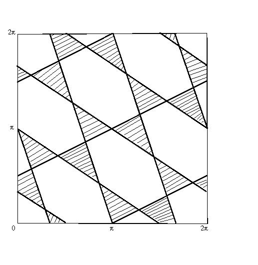
Figure 1. The coamoeba of the curve defined by the polynomial $f_{1}(z,w)=wz^{3}+z^{2}w^{3}+1$

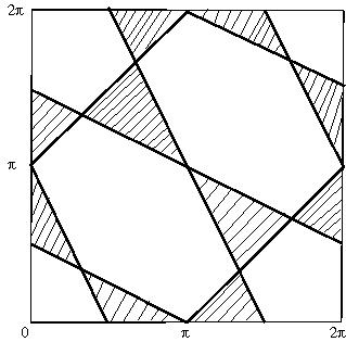
Figure 2. The coamoeba of the curve defined by the polynomial $f(z,w)=z+w+z^{2}w^{2}$

4. Tropical mirror hypersurfaces

Let $V_{f}\subset(\mathbb{K}^{*})^{n}$ be an algebraic hypersurface defined by a polynomial $f$ and we assume that $\Delta_{f}$ is a simplex, $A=\mathop{\rm Vert}\nolimits(\Delta_{f})\cup\{\beta\}$, and the coefficient $a_{\beta}$ is monomial. In addition, we suppose that $\beta\in\mathop{\rm Vert}\nolimits(\tau_{f})$. Let $\displaystyle{\{f_{u}\}_{u\in]-1;1]}}$ be the family of polynomials defined as follow:

$$f_{u}(z)=a_{\beta,\,u}z^{\beta}+\sum_{\alpha\in\mathop{\rm Vert}\nolimits(\Delta_{f})}a_{\alpha}z^{\alpha},$$

with $a_{\beta,\,u}$ such that:

$$a_{\beta,\,u}=\left\{\begin{array}[]{ll}\xi_{\beta}t^{u\nu_{f}(\beta)+(1-u)(<\beta,v>+r)}&\mbox{if\, $u\in[0;1]$}\\ \xi_{\beta}t^{(1-u)(<\beta,v>+r)-\frac{u}{u+1}}&\mbox{if\, $u\in]-1;0]$}\end{array}\right.$$

where $\xi_{\beta}$ is the complex coefficient of $a_{\beta}$, and $v$ is the vertex of the tropical hypersurface $\mathop{\rm Val}\nolimits(V_{f})$. We can assume that $<\beta,v>+r\geq 0$ (multiplying $f$ by a power of $t$ if necessary); so the map $u\longmapsto(1-u)(<\beta,v>+r)-\frac{u}{u+1}$ is a decreasing function on $]-1;0]$.

Remark 4.1.

• The deformation given above is such that $f_{1}(z)=f(z)$;

• for any $u\in]-1;0]$, the subdivision $\tau_{f_{u}}=\{\Delta_{f}\}$ (i.e., trivial);

• with the same assumption as above, when the order of the monomial $a_{\beta,\,u}$ reaches the hyperplane of $\mathbb{R}^{n}\times\mathbb{R}$ containing the points with coordinates $(\alpha,\nu_{f}(\alpha))$ and $\alpha\in\mathop{\rm Vert}\nolimits(\Delta_{f})$ (i.e., for $u\leq 0$). Then we consider the family of polynomials $\tilde{f}_{u}$ defined by:

  $$\tilde{f}_{u}(z)=\tilde{a}_{\beta,\,u}z^{-\beta}+\sum_{\alpha\in\mathop{\rm Vert}\nolimits(\Delta_{f})}\tilde{a}_{\alpha}z^{-\alpha},$$

  such that if   $\alpha\in\mathop{\rm Vert}\nolimits(\Delta_{f})$ and $\displaystyle{a_{\alpha}(t)=\sum_{r\geq\mathop{\rm ord}\nolimits(a_{\alpha})}\xi_{\alpha,r}t^{r}}$, then we set $\displaystyle{\tilde{a}_{\alpha}(t)=}$
  $\displaystyle{\sum_{r\geq\mathop{\rm ord}\nolimits(a_{\alpha})}\xi_{\alpha,r}t^{-r}}$ and if  $a_{\beta,\,u}(t)=\xi_{\beta}t^{\mathop{\rm ord}\nolimits(a_{\beta,\,u})}$, we set   $\tilde{a}_{\beta,\,u}(t)=\xi_{\beta}t^{-\mathop{\rm ord}\nolimits(a_{\beta,\,u})}$. In this case, we have the convergence when $t$ tends to the infinity, because the induced transformation of $\mathbb{K}$ is given by $t\longmapsto t^{-1}$. Let $\mathscr{I}:(\mathbb{K}^{*})^{n}\rightarrow(\mathbb{K}^{*})^{n}$ be the transformation defined as $(z_{1},\ldots,z_{n})\mapsto(z_{1}^{-1},\ldots,z_{n}^{-1})$, then by making the change of the variable $t=\frac{1}{\tau}$, we can see that $\tilde{f}_{u}(z)=f_{u}\circ\mathscr{I}(z)$, and then $V_{\tilde{f}_{u}}=V_{f_{u}\circ\mathscr{I}}=\mathscr{I}(V_{f_{u}})$. The tropical polynomial associated to $\tilde{f}_{u}$ is given by

  $$\tilde{f}_{u,\,trop}=\max_{\alpha\in\mathop{\rm Sym}\nolimits(A)}\{<x,\gamma>-\mathop{\rm val}\nolimits(a_{\gamma,u})\}$$

  with $\mathop{\rm Sym}\nolimits(A)$ the subset of $\mathbb{Z}^{n}$ symmetric to $A$ relatively to the origin. There exist a positive number $s\in]-1;0]$ such that the non-Archimedean amoebas defined by the tropical polynomials $\tilde{f}_{u,\,trop}$ with $u\in[-s;0]$ are symmetric to those defined by $f_{u,\,trop}$ with $u\in[0;1]$ (By an automorphism of $(\mathbb{K}^{*})^{n}$ if necessary, we can assume that $\mathop{\rm val}\nolimits(a_{\alpha})=0$ for any $\alpha\in\mathop{\rm Vert}\nolimits(\Delta_{f}$, and in this case $s=-\nu_{f}(a_{\beta})$.). So, we can apply now Kapranov’s theorem to the tropical hypersurfaces $\Gamma_{\tilde{f}_{u}}$, and from the equality $V_{\tilde{f}_{u}}=\mathscr{I}(V_{f_{u}})$, we deduced that the coamoeba of $V_{\infty,\,f_{u}}=W(V_{f_{u}})$ is the symmetric of the coamoeba of $V_{\infty,\,\tilde{f}_{u}}=W(V_{\tilde{f}_{u}})$.

• One way to look at the deformation of a tropical hypersurface is to think of it as a deformation of the extending Newton polytope of its defining polynomial. More precisely, the deformation $\tilde{f}_{u,\,trop}$ can be seen as a continuation of the deformation of the normal vectors to the hyperplanes in $\mathbb{R}^{n}\times\mathbb{R}$ containing the lifting of the $\Delta_{i}$’s element of the subdivision $\tau_{f_{u}}$ dual to ${f}_{u,\,trop}$ with $0\leq u\leq 1$. Indeed, when $u=0$, all the normal vectors are equal and then for $u\leq 0$ the coefficient of index $\beta$ becomes inessential in the tropical polynomial ${f}_{u,\,trop}$, but in the non-Archimedean polynomial $f_{u}$, it has a contribution and plays a crucial role for the determination of the complex tropical hypersurface coamoeba.

Definition 4.2.

The tropical hypersurfaces $\mathop{\rm Val}\nolimits(V_{\tilde{f}_{u}})$ defined by the tropical polynomials $\tilde{f}_{u,\,trop}$ for $u\in]-1;0]$, are called the tropical mirror for the hypersurfaces $V_{f_{u}}$ defined by the polynomial $f_{u}$. We denote this hypersurface by $\mathop{\rm Mirr}\nolimits_{trop}(V_{f_{u}}):=\mathop{\rm Val}\nolimits(V_{\tilde{f}_{u}})$.

We can see that if $\Gamma$ is a tropical hypersurface with only one vertex, and $V_{1},V_{2}$ are two hypersurfaces in $(\mathbb{K}^{*})^{n}$ such that $\mathop{\rm Val}\nolimits(V_{i})=\Gamma$ for $i=1,2$, then the two mirror tropical hypersurfaces $\mathop{\rm Mirr}\nolimits_{trop}(V_{1})$ and $\mathop{\rm Mirr}\nolimits_{trop}(V_{2})$ are not necessary the same. A similar algebraic construction is given by Z. Izhakian and L. Rowen in [IR-08].

Theorem 4.3.

Let $V_{f}\subset(\mathbb{K}^{*})^{n}$ be a hypersurface defined by a polynomial $f$ with Newton polytope $\Delta$, and assume that the subdivision $\tau_{f}=\{\Delta_{1},\ldots,\Delta_{l}\}$ dual to the tropical hypersurface $\mathop{\rm Val}\nolimits(V_{f})$ is a triangulation. Then the geometry and the topology of the complex tropical hypersurfaces $W(V_{f})$ coamoebas are completely determined and constructed by gluing those of the truncated complex tropical hypersurfaces $W(V_{f^{\Delta_{i}}})$ using the complex tropical localization.

Proof   Suppose that $V_{f}\subset(\mathbb{K}^{*})^{n}$ is defined by the polynomial $\displaystyle{f(z)=\sum_{\alpha\in A}a_{\alpha}z^{\alpha}}$ with Newton polytope $\Delta$ equal to the convex hull of $A$, and let $A_{i}=A\cap\Delta_{i}$. If $f^{\Delta_{i}}$ denotes the truncation of $f$ to $\Delta_{i}$, then the assumption of Theorem 4.3, means that the spine of the hypersurface amoeba of $V_{f^{\Delta_{i}}}$ has only one vertex. Let $\tau_{i}=\cup_{j}\Delta_{ij}$ be the convex subdivision of $\Delta_{i}$ given by taking the upper bound of the convex hull of the set $\{(\alpha,r)\in A_{i}\times\mathbb{R}\mid r\leq\mathop{\rm ord}\nolimits(a_{\alpha})\}$, which we can suppose to be a triangulation (by a small perturbation of the coefficients order if necessary). Let $inv:\mathbb{C}((t))\rightarrow\mathbb{C}((\rho))$ be the morphism sending $t$ of valuation $+1$ to $\rho$ of valuation $-1$, and let $\tilde{f}$ be the polynomial defined by $\displaystyle{\tilde{f}(z)=\sum_{\alpha\in A_{i}}\tilde{a}_{\alpha}z^{-\alpha}}$ with $\tilde{a}_{\alpha}=inv(a_{\alpha})$ (this means that if $\displaystyle{a_{\alpha}(t)=\sum_{r\geq\mathop{\rm ord}\nolimits(a_{\alpha})}\xi_{\alpha,r}t^{r}}$ then $\displaystyle{\tilde{a}_{\alpha}(t)=\sum_{r\geq\mathop{\rm ord}\nolimits(a_{\alpha})}\xi_{\alpha,r}t^{-r}}$). We use now induction on the volume of $\Delta$, and we assume that the coamoeba of any $V_{f^{\Delta_{ij}}}$ is constructed for each index $ij$ using the complex tropical localization which we develop in the next section. By construction we have $V_{\tilde{f}_{i}}=V_{f^{\Delta_{i}}\circ\mathscr{I}}=\mathscr{I}(V_{f^{\Delta_{i}}})$. The coamoeba of $V_{\tilde{f}_{i}}$ can be constructed, because in this case, one can apply Kapranov’s Theorem, and we can also build the coamoeba of $V_{f^{\Delta_{i}}}$. Knowing now all the coamoebas of the $V_{f^{\Delta_{i}}}$’s, the coamoeba of the hypersurface $V_{f}$ itself can be built by reusing Kapranov’s Theorem.  

Examples 4.4.

• Example of the parabola (see figures 3, 4, and 5), where the deformation is seen as a deformation of the normal vectors to the hyperplanes in $\mathbb{R}^{n}\times\mathbb{R}$ containing the lifting of the $\Delta_{i}$’s, and the points with coordinates $(\alpha,\mathop{\rm ord}\nolimits(\alpha))$ and $\alpha\in\mathop{\rm Vert}\nolimits(\Delta_{f})$ are fixed.

  

  

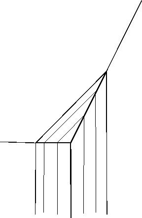
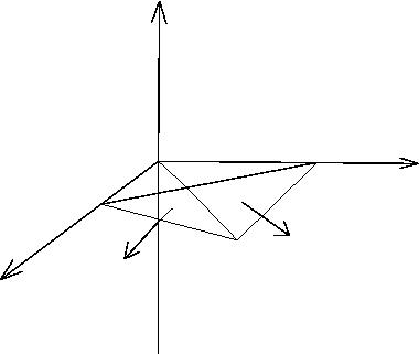
  Figure 3. The tropical curves $\mathop{\rm Val}\nolimits(V_{f_{u}})$ for $u\in[0;1]$.

  

  

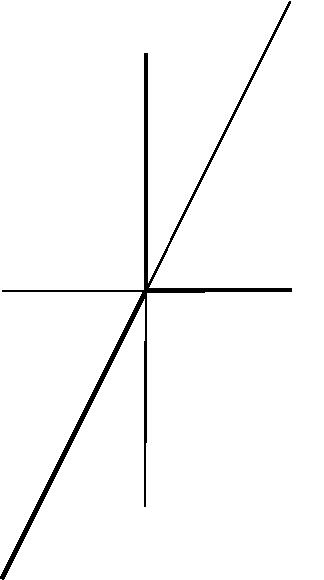
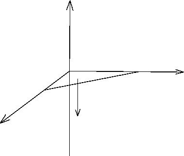
  Figure 4. The tropical curves $\mathop{\rm Val}\nolimits(V_{f_{0}})$ and $\mathop{\rm Val}\nolimits(V_{\tilde{f}_{0}})$.

  

  

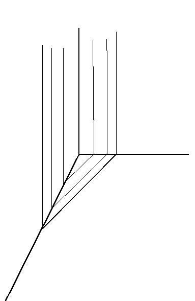
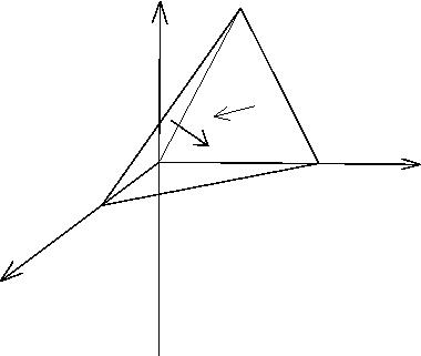
  Figure 5. The tropical curves $\mathop{\rm Val}\nolimits(V_{\tilde{f}_{u}})$ for $u\in]-1;0]$.

• We give here an example where $\beta\in\mathop{\rm Int}\nolimits(\Delta_{f})$ (see figures 6, 7, and 8), and as in the previous example, the deformation is supposed to fix the order of the coefficients of index in the vertices of the Newton polygon.

  

  

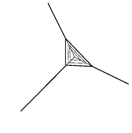
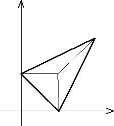
  Figure 6. The tropical curves $\mathop{\rm Val}\nolimits(V_{f_{u}})$ for $u\in[0;1]$.

  

  

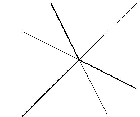
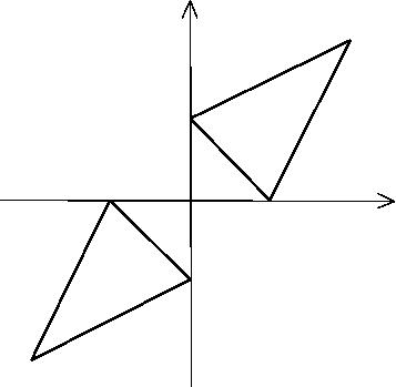
  Figure 7. The tropical curves $\mathop{\rm Val}\nolimits(V_{f_{0}})$ and $\mathop{\rm Val}\nolimits(V_{\tilde{f}_{0}})$.

  

  

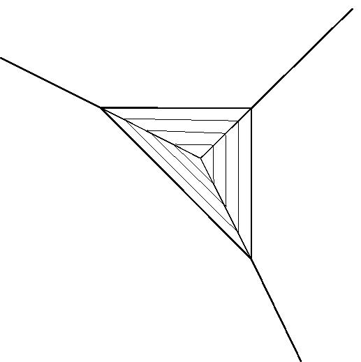
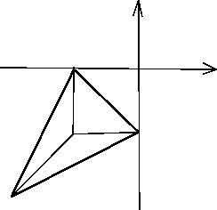
  Figure 8. The tropical curves $\mathop{\rm Val}\nolimits(V_{\tilde{f}_{u}})$ for $u\in]-1;0]$.

5. Camoebas of complex tropical hypersurfaces

In this section we consider an algebraic hypersurface $V$ over the field of Puiseux series $\mathbb{K}$ defined by a polynomial $f$ with Newton polytope $\Delta$. We denote by $\Gamma$ the non-Archimedean amoeba of $V$ and by $V_{\infty,\,f}$ the complex tropical hypersurface image of $V$ under the map $W$. Let us denote by $\tau$ the subdivision of $\Delta$ dual to $\Gamma$ which we suppose to be a triangulation, and assume that $f$ is defined as follows:

$$f(z)=\sum_{\alpha\in\mathop{\rm supp}\nolimits(f)}a_{\alpha}z^{\alpha},\,\,\,\,\quad\quad\quad z^{\alpha}=z_{1}^{\alpha_{1}}z_{2}^{\alpha_{2}}\ldots z_{n}^{\alpha_{n}},$$

where $a_{\alpha}$ are non-zero complex Puiseux series and $\mathop{\rm supp}\nolimits(f)$ is the support of $f$.

5.1. Complex tropical localization

Definition 5.2.

Let $\mathbb{R}^{n}$ be the universal covering of the real torus $(S^{1})^{n}$. Let $\alpha$ and $\beta$ be in the support of $f$. A hypersurface $H_{\alpha\beta}\subset\mathbb{R}^{n}$ is called codual (or corresponding) to an edge $E_{\alpha\beta}$ in $\tau$ if it is given by the following equation:

$$\arg(a_{\alpha})-\arg(a_{\beta})+<\alpha-\beta,x>=\pi.$$

In addition if $E_{\alpha\beta}$ is an external edge of $\tau$ (i.e., $E_{\alpha\beta}$ is a proper edge of the Newton polytope $\Delta$), then $H_{\alpha\beta}$ is called an external hyperplane.

Definition 5.3.

An open subset $\mathcal{C}$ of the coamoeba of a complex tropical hypersurface $V_{\infty,\,f}$ is called regular if for any point $x$ in $\mathcal{C}$ there exist an open subset $V(x)$ in $(S^{1})^{n}$ containing $x$ with $V(x)\subset\mathcal{C}$ and an open subset $U$ in $\mathbb{R}^{n}$ such that $V(x)\subset\mathop{\rm Arg}\nolimits(\mathop{\rm Log}\nolimits^{-1}(U)\cap V_{\infty,\,f})_{i}$ where $(\mathop{\rm Log}\nolimits^{-1}(U)\cap V_{\infty,\,f})_{i}$ is one connected component of $\mathop{\rm Log}\nolimits^{-1}(U)\cap V_{\infty,\,f}$.

We denote by $\mathop{\rm Critv}\nolimits(\mathop{\rm Arg}\nolimits)$ the set of critical values points in the coamoeba $co\mathscr{A}$ of a complex tropical hypersurface $V$.

Definition 5.4.

An extra-piece is a connected component $\mathcal{C}$ of $co\mathscr{A}\setminus\mathop{\rm Critv}\nolimits(\mathop{\rm Arg}\nolimits)$ such that the boundary of its closure $\partial\,\overline{\mathcal{C}}$ is not contained in the union of hyperplanes codual to the edges of the subdivision.

This means that its boundary contains at least one component (smooth) in the set of critical values of the argument map. In the following Lemma we assume that the subdivision $\tau$ of the Newton polytope $\Delta$ dual to the non-Archimedean amoeba $\Gamma$ is a triangulation and contains inner edges.

We begin by proving the following Lemma which is a local version of the Theorem 6.1 in the complex tropical case.

Lemma 5.5.

Let $H_{\alpha\gamma}$ be a hyperplane in $\mathbb{R}^{n}$ codual to an inner edge $E_{\alpha\gamma}$ of the subdivision $\tau$. Then any connected component $\mathcal{C}$ of $H_{\alpha\gamma}\cap\mathop{\rm Arg}\nolimits(V_{\infty,\,f})$ has a dimension $n-1$ and its interior is contained in the interior of a regular part of $\mathop{\rm Arg}\nolimits(V_{\infty,\,f})$.

Proof   Let $\Delta_{1}$ and $\Delta_{2}$ be two elements of $\tau$ with a common edge $E_{\alpha\gamma}$, and $v_{1}$ and $v_{2}$ be their dual vertices in the non-Archimedean amoeba $\Gamma$. Let $\{x_{m}\}$ be a sequence in $\mathop{\rm Arg}\nolimits(\mathop{\rm Log}\nolimits^{-1}(v_{1})\cap V_{\infty,\,f^{\Delta_{1}}})\setminus\mathop{\rm Arg}\nolimits(\mathop{\rm Log}\nolimits^{-1}(v_{2})\cap V_{\infty,\,f^{\Delta_{2}}})$ which converge to some point $x$ in $H_{\alpha\gamma}\setminus\mathop{\rm Arg}\nolimits(\mathop{\rm Log}\nolimits^{-1}(v_{2})\cap V_{\infty,\,f^{\Delta_{2}}})$. Let $\mathscr{C}$ be a connected component of $\mathop{\rm Arg}\nolimits^{-1}(\{x_{m}\})\cap V_{\infty,\,f}$ and $\{z_{m}\}\subset\mathscr{C}$ be a sequence such that $\mathop{\rm Arg}\nolimits(z_{m})=x_{m}$ for each $m$. We claim that the sequence $\{z_{m}\}$ (by taking a subsequence if necessary) converges to some point $z$ in $V_{\infty,\,f}$. Indeed, the sequence $\{\mathop{\rm Log}\nolimits(z_{m})\}$ converge to $v_{2}$ because the argument of $z_{m}$ is $x_{m}$ which converges to $x\in H_{\alpha\gamma}$, and $x$ is an infinite point for $\mathop{\rm Arg}\nolimits(V_{\infty,\,f^{\Delta_{1}}})$. This means that $\{\mathop{\rm Log}\nolimits(z_{m})\}$ converges asymptotically in the direction of $E_{\alpha\gamma}$ to the infinity of $\mathop{\rm Log}\nolimits(V_{\infty,\,f^{\Delta_{1}}})$. So $z_{m}$ converge to the point $z$ of $(\mathbb{C}^{*})^{n}$ with argument $x$ and the valuation $v_{2}$. $V_{\infty,\,f}$ is closed, hence $z\in V_{\infty,\,f}$. Then all the components of $H_{\alpha\gamma}\setminus\left(\overline{\mathop{\rm Arg}\nolimits(\mathop{\rm Log}\nolimits^{-1}(v_{1})\cap V_{\infty,\,f^{\Delta_{1}}})}\cap\overline{\mathop{\rm Arg}\nolimits(\mathop{\rm Log}\nolimits^{-1}(v_{2})\cap V_{\infty,\,f^{\Delta_{2}}})}\right)$ are in the interior of $\mathop{\rm Arg}\nolimits(V_{\infty,\,f})$. Let now $x$ be a point in the interior of the following set:

$$H_{\alpha\gamma}\cap\left(\overline{\mathop{\rm Arg}\nolimits(\mathop{\rm Log}\nolimits^{-1}(v_{1})\cap V_{\infty,\,f^{\Delta_{1}}})}\cap\overline{\mathop{\rm Arg}\nolimits(\mathop{\rm Log}\nolimits^{-1}(v_{2})\cap\mathop{\rm Arg}\nolimits(V_{\infty,\,f^{\Delta_{2}}})}\right),$$

and $\{x_{m}\}$ be a sequence in $\mathop{\rm Arg}\nolimits(\mathop{\rm Log}\nolimits^{-1}(v_{1})\cap V_{\infty,\,f^{\Delta_{1}}})\cap\mathop{\rm Arg}\nolimits(\mathop{\rm Log}\nolimits^{-1}(v_{2})\cap\mathop{\rm Arg}\nolimits(V_{\infty,\,f^{\Delta_{2}}})$ such that $x_{m}$ converges to $x$. We claim that there is no sequence $\{z_{m}\}$ in $V_{\infty,\,f}$ such that $\mathop{\rm Arg}\nolimits(z_{m})=x_{m}$ for any $m$ and $z_{m}$ converges in $V_{\infty,\,f}$ to some point $z$ such that $\mathop{\rm Arg}\nolimits(z)=x$. Indeed, assume on the contrary that there exists a sequence $\{z_{m}\}$ in $V_{\infty,\,f}$ satisfying the assumption and converging to $z$ in $V_{\infty,\,f}$. On one hand we know that $\mathop{\rm Log}\nolimits(z_{m})$ converges to $v_{2}$, because the argument of $z_{m}$ converges to $x\in H_{\alpha\gamma}$ which is an infinite point for $\mathop{\rm Arg}\nolimits(\mathop{\rm Log}\nolimits^{-1}(v_{1})\cap V_{\infty,\,f^{\Delta_{1}}})$ and then the valuation of the $z_{m}$’s tends to the infinity asymptotically in the direction of $E_{\alpha\gamma}$ to $v_{2}$ (because $v_{2}$ represents the infinity for $\mathop{\rm Log}\nolimits(V_{\infty,\,f^{\Delta_{1}}})$ in the direction of $E_{\alpha\gamma}$). On the other hand, for the same reasons, the sequence $\mathop{\rm Log}\nolimits(z_{m})$ converge to $v_{1}$. Contradiction, because by assumption $v_{1}\neq v_{2}$. In this case we have the so-called extra-piece.  

Proposition 5.6.

Let $H_{\alpha\gamma}$ be a hyperplane in $\mathbb{R}^{n}$ codual to an external edge $E_{\alpha\gamma}$ of the subdivision $\tau$, and let $\mathcal{C}$ be a connected component of $H_{\alpha\gamma}\cap\mathop{\rm Arg}\nolimits(V_{\infty,\,f})$. Then we have one of the two following cases:

• The dimension of $\mathcal{C}$ is $n-1$ and its interior is contained in the interior of a regular part of $\mathop{\rm Arg}\nolimits(V_{\infty,\,f})$;

• the dimension of $\mathcal{C}$ is zero (i.e., discrete) and $\mathcal{C}$ is contained in the intersection of $H_{\alpha\gamma}$ and a line codual to some proper face of $\Delta_{v}$.

If the edge $E_{\alpha\gamma}$ is a common edge to more than one element of the subdivision $\tau$ (which can occur only if $n>2$), then by Lemma 5.5 we have the first case. Assume that $E_{\alpha\gamma}$ is an edge of only one element $\Delta_{v}$ of $\tau$, and we denote by $v$ the vertex of the tropical hypersurface dual to $\Delta_{v}$. Let $z\in\mathop{\rm Log}\nolimits^{-1}(v)\cap V_{\infty,\,f}$ such that $\mathop{\rm Arg}\nolimits(z)=x$ which we assume in $H_{\alpha\gamma}$. We denote by $\mathcal{C}$ the connected component of $H_{\alpha\gamma}\cap\mathop{\rm Arg}\nolimits(V_{\infty,\,f})$ containing $x$. We have to consider the following cases:

• $\mathop{\rm supp}\nolimits(f)=\mathop{\rm Vert}\nolimits(\Delta_{v})$, in this case there is nothing to prove, and we have case (ii) of the Proposition.

• $\mathop{\rm supp}\nolimits(f)\cap\Delta_{v}=\mathop{\rm Vert}\nolimits(\Delta_{v})$ or $\mathop{\rm supp}\nolimits(f)=\mathop{\rm Vert}\nolimits(\Delta_{v})\cup\{\beta_{1},\ldots,\beta_{l}\}$ with $\beta_{j}\in\Delta_{v}\cap\mathbb{Z}^{n}$ for any $j$.

All other cases will be easily deduced thereof. Assume that $\mathop{\rm supp}\nolimits(f)=\mathop{\rm Vert}\nolimits(\Delta_{v})\cup\{\beta\}$ with $\beta\in\Delta_{v}$.

Lemma 5.7.

With the above notations, let $A$ be the interior of $\mathcal{C}$, then for any $x\in A$ there exists an open neighborhood $\mathscr{V}(x)$ of $x$ in $(S^{1})^{n}$ such that $\mathscr{V}(x)\subset\mathop{\rm Arg}\nolimits(V_{\infty,\,f})$.

Proof   Indeed, assume on the contrary that there exists a small open neighborhood $\mathscr{V}(x)$ of $x$ in $\mathbb{R}^{n}$ such that $\mathscr{V}(x)\cap co\mathscr{A}_{f^{\Delta_{\alpha_{j}}}}$ is empty, where $\Delta_{\alpha_{j}}$ is the simplex with vertices $\{\alpha_{1},\ldots,\widehat{\alpha_{j}},\ldots,\alpha_{n+1},\beta\}$ and $E_{\alpha\gamma}=E_{\alpha_{1}\alpha_{2}}$ with $j\neq 1,2$ (here we use the same letter for $x$ and its lifting to the universal covering of the torus; abuse of notation). This means that $\mathscr{V}(x)\cap\mathop{\rm Arg}\nolimits(V_{\infty,\,f})$ lies in one side of the hyperplane $H_{\alpha_{1}\alpha_{2}}$. So the dominating monomials in $W^{-1}(\mathop{\rm Arg}\nolimits^{-1}(\mathscr{V}(x))\cap V_{\infty,\,f})$ are $a_{\alpha_{1}},\widehat{a_{\alpha_{2}}},\ldots,a_{\alpha_{n+1},\beta}$, because if the monomial $a_{\alpha_{2}}$ is a dominating one, then $\mathop{\rm Arg}\nolimits(V_{\infty,\,f})\cap\mathscr{V}(x)$ lies on both sides of $H_{\alpha_{1}\alpha_{2}}$. From Remarks 4.1 (a), (b), (c) and Kapranov’s Theorem [K-00], we obtain that the dominating monomials in $W^{-1}(\mathop{\rm Log}\nolimits^{-1}(v)\cap V_{\infty,\,f})$ are $a_{\alpha_{1}},a_{\alpha_{2}},\ldots,a_{\alpha_{n+1}}$. Hence $z$ lies in the domain where the monomials $a_{\alpha_{1}},\widehat{a_{\alpha_{2}}},\ldots,a_{\alpha_{n+1}}$ are dominating (a proper face of the simplex $\Delta_{v}$), and then $\mathop{\rm Arg}\nolimits(z)=x$ is contained in $H_{\alpha_{1}\alpha_{2}}\cap\mathop{\rm Arg}\nolimits(V_{\infty,\,f^{\Delta_{\alpha_{2}}}})$. Contradiction, because $H_{\alpha_{1}\alpha_{2}}\cap\mathop{\rm Arg}\nolimits(V_{\infty,\,f^{\Delta_{\alpha_{2}}}})$ is discrete and then the intersection of any open neighborhood of $x$ in $\mathbb{R}^{n}$ with $\mathop{\rm Arg}\nolimits(V_{\infty,\,f})$ lies on both sides of the hyperplane $H_{\alpha_{1}\alpha_{2}}$. In this case we have some extra-piece.

 

Theorem 1.1 is an immediate consequence of Lemma 5.5 and Proposition 5.6.

6. Coamoebas of complex algebraic hypersurfaces

We now turn our attention to complex algebraic hypersurfaces, so in this section we assume that the polynomial $f$ is complex. We will give a caracterization of the argument map critical values set contained in the hyperplanes codual to the edges of the subdivision $\tau$ dual to the spine of the amoeba $\mathscr{A}$ of $V_{f}$, and we have the following.

Theorem 6.1.

Let $H_{\alpha\gamma}$ be a hyperplane in $\mathbb{R}^{n}$ codual to an edge $E_{\alpha\gamma}$. Then the intersection $H_{\alpha\gamma}\cap\mathop{\rm Critv}\nolimits(\mathop{\rm Arg}\nolimits)$ is discrete and it is contained in the union of lines $L_{\alpha^{\prime}\beta^{\prime}}$ codual to some faces of $\tau$.

Proof   Assume that there is an open subset $A$ of $H_{\alpha\gamma}$ such that $A\subset co\mathscr{A}_{V_{f}}$, then we claim that $A\subset co\mathscr{A}_{V_{\infty,\,f}}$. Indeed, assume that $E_{\alpha\gamma}$ is a common edge for two simplices $\Delta_{1}$ and $\Delta_{2}$. Let $y=<x,a_{1}>+b_{1}$ be the equation of the hyperplane in $\mathbb{R}^{n}\times\mathbb{R}$ containing the points with coordinates $(\alpha,\nu(\alpha))$ and $\alpha\in\mathop{\rm Vert}\nolimits(\Delta_{1})$ and $\nu$ the Passare-Rullgård function. Let $\displaystyle{f_{t}(z)=\sum a_{\alpha}(et)^{<\alpha,a_{1}>+b_{1}}z^{\alpha}}=(et)^{b_{1}}\sum a_{\alpha}((et)^{a_{1}}z)^{\alpha}$ with $a_{1}=(a_{11},\ldots,a_{1n})$ and

$$((et)^{a_{1}}z)^{\alpha}=(et)^{a_{11}{\alpha_{1}}}z_{1}^{\alpha_{1}}(et)^{a_{12}{\alpha_{2}}}z_{2}^{\alpha_{2}}\ldots(et)^{a_{1n}{\alpha_{n}}}z_{n}^{\alpha_{n}}.$$

Hence $V_{f_{t}}\subset(\mathbb{C}^{*})^{n}$ is the image of $V_{f}$ under the self diffeomorphism $\phi_{t}$ of $(\mathbb{C}^{*})^{n}$ given by:

$$(z_{1},\ldots,z_{n})\mapsto((et)^{a_{11}}z_{1},(et)^{a_{12}}z_{2},\ldots,(et)^{a_{1n}}z_{n})$$

which conserves the arguments. Assume now that $A\subset co\mathscr{A}_{V_{f}}\cap\mathop{\rm Critv}\nolimits(\mathop{\rm Arg}\nolimits)$, so when $t$ is so close to zero then the set $\mathop{\rm Log}\nolimits(\mathop{\rm Arg}\nolimits^{-1}(A)\cap V_{f})$ take place on the two sides of the hyperplane $E^{*}_{\alpha\gamma}$ in $\Gamma$ dual to $E_{\alpha\gamma}$, because it is the case for the truncation $V_{f^{\Delta_{1}}}$ which approximate our hypersurface when $t$ tends to zero. So, if one chooses a coefficients $d_{\alpha}$ and $d_{\gamma}$ such that the holomorphic annulus $\mathscr{Y}$ of equation $d_{\alpha}z^{\alpha}+d_{\gamma}z^{\gamma}=0$ has the hyperplane containing $E^{*}_{\alpha\gamma}$ as its amoeba, and the hyperplane $H_{\alpha\gamma}$ as its coamoeba, then $V_{f}\cap\mathscr{Y}$ is nonempty. Let $z_{0}$ be a point in $V_{f}\cap\mathscr{Y}$, hence $\phi_{t}^{-1}(z_{0})\in\phi_{t}^{-1}(V_{f})\cap\phi_{t}^{-1}(\mathscr{Y})$ and then $\mathop{\rm Arg}\nolimits(z_{0})\in co\mathscr{A}_{V_{\infty,\,f^{\Delta_{1}}}}$. It contradicts Lemma 5.5 if the hyperplane $H_{\alpha\gamma}$ is inner, and Proposition 5.6 if $H_{\alpha\gamma}$ is external, and then $A$ is contained in the interior of a regular part of the coamoeba or it is discrete.  

Let $t$ be a strictly positive real number in $\in]0;\frac{1}{e}]$, and $H_{t}$ be the following self diffeomorphism of $(\mathbb{C}^{*})^{n}$:

$$\begin{array}[]{ccccl}H_{t}&:&(\mathbb{C}^{*})^{n}&\longrightarrow&(\mathbb{C}^{*})^{n}\\ &&(z_{1},\ldots,z_{n})&\longmapsto&(\parallel z_{1}\parallel^{-\frac{1}{\log t}}\frac{z_{1}}{\parallel z_{1}\parallel},\ldots,\parallel z_{n}\parallel^{-\frac{1}{\log t}}\frac{z_{n}}{\parallel z_{n}\parallel}).\end{array}$$

which defines a new complex structure on $(\mathbb{C}^{*})^{n}$ denoted by $J_{t}=(dH_{t})\circ J\circ(dH_{t})^{-1}$ where $J$ is the standard complex structure. A $J_{t}$-holomorphic hypersurface $V_{t}$ is a hypersurface holomorphic with respect to the $J_{t}$ complex structure on $(\mathbb{C}^{*})^{n}$. It is equivalent to say that $V_{t}=H_{t}(V)$ where $V\subset(\mathbb{C}^{*})^{n}$ is an holomorphic hypersurface with respect to the standard complex structure $J$ on $(\mathbb{C}^{*})^{n}$.

Recall that the Hausdorff distance between two closed subsets $A,B$ of a metric space $(E,d)$ is defined by:

$$d_{\mathcal{H}}(A,B)=\max\{\sup_{a\in A}d(a,B),\sup_{b\in B}d(A,b)\}.$$

Here we take $E=\mathbb{R}^{n}\times(S^{1})^{n}$, with the distance defined as the product of the Euclidean metric on $\mathbb{R}^{n}$ and the flat metric on $(S^{1})^{n}$.

A complex tropical hypersurface can be defined as follows (see [M1-02] and [M2-04]).

Definition 6.2.

A complex tropical hypersurface $V_{\infty}\subset(\mathbb{C}^{*})^{n}$ is the limit when $t$ tends to zero of a sequence of a $J_{t}$-holomorphic hypersurfaces $V_{t}\subset(\mathbb{C}^{*})^{n}$ (with respect to the Hausdorff metric on compact sets in $(\mathbb{C}^{*})^{n}$).

6.3. Coamoebas of maximally sparse hypersurfaces

Let $V_{f}\subset(\mathbb{C}^{*})^{n}$ be a hypersurface   defined by a maximally sparse polynomial $\displaystyle{f(z)=}$
$\displaystyle{\sum_{\alpha\in\mathop{\rm Vert}\nolimits(\Delta_{f})}a_{\alpha}z^{\alpha}}$ (recall that a polynomial $f$ is maximally sparse means that $\mathop{\rm supp}\nolimits(f)=\mathop{\rm Vert}\nolimits(\Delta_{f})$). Let $f_{t}$ be the family of polynomials defined by
$\displaystyle{f_{t}(z)=\sum_{\alpha\in\mathop{\rm Vert}\nolimits(\Delta_{f})}a_{\alpha}(et)^{-\mathop{\rm Log}\nolimits(a_{\alpha})}z^{\alpha}}$ and $V_{t}$ their zero locus. We denote by $\displaystyle{V_{\infty,\,f}=\lim_{t\rightarrow 0}H_{t}(V_{t})}$ with respect to the Hausdorff metric on compact sets of $(\mathbb{C}^{*})^{n}$.

Theorem 6.4.

With the above notations and assumptions, the deformation of $V_{f}$ given by the family of polynomials $f_{t}$ satisfies the following: the coamoeba of the complex tropical hypersurface $V_{\infty,\,f}$ has the same topology of the coamoeba $co\mathscr{A}_{f}$ of $V_{f}$ (i.e., they are homeomorphic).

Proof   We will prove that the deformation given by $\{f_{t}\}$ defines a bijection between the complement components of the $V_{f}$’s coamoeba and the complement components of the $V_{\infty,\,f}$’s coamoeba. More precisely, we prove that such deformation conserve the complement components of the coamoeba and thus its topology. Assume that a complement component of the coamoeba is created (resp. disappear) for some $t$. Then there is a created (resp. disappear) component of the argument map critical values boundary, it means that some edge of the subdivision $\tau_{f}$ dual to the spine of the amoeba $\mathscr{A}_{f}$ disappears (resp. created), but it cannot occur because the polynomials are maximally sparse, and thus, the spines of the amoebas $\mathscr{A}_{V_{f_{t}}}$ are of the same combinatorial type. It remains to show that two different complement components of the $V_{f}$’s coamoeba cannot be deformed to the same complement component of the $V_{\infty,\,f}$’s coamoeba. Assume on the contrary that there is two complement components $\mathcal{C}_{1}$ and $\mathcal{C}_{2}$ of the $V_{f}$’s coamoeba which are deformed to one complement component $\mathcal{C}$ of the $V_{\infty,\,f}$’s coamoeba. It means that one of these two components disappears or the component $\mathcal{C}$ is not convex, and then we have a contradiction in both cases.

 

7. Examples of complex algebraic plane curves coamoebas

• Let $V_{f_{\lambda}}$ be the curve in $(\mathbb{C}^{*})^{2}$ defined by the following polynomial:

  $$f_{\lambda}(z,w)=w^{2}-\lambda w+2zw-z^{2}w+1.$$

  Let $f_{\lambda,\,1}(z,w)=w^{2}-\lambda w+2zw-z^{2}w$, so $V_{f_{\lambda,\,1}}$ is just the parabola of example 1. Let $f_{\lambda,\,2}(z,w)=-\lambda w+2zw-z^{2}w+1$, hence $V_{f_{\lambda,\,2}}$ is the set of points $(z,w)\in(\mathbb{C}^{*})^{2}$ such that :

  $$w=\frac{1}{z^{2}-2z+\lambda}.$$

  This means that $\arg(w_{2})=-\arg(w_{1})$ mod $2\pi$. Hence the coamoeba of the curve defined by $f_{\lambda}$ is as in the figure 8 on the left.

  

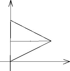
  Figure 9. The Newton Polygon of example (1) and its subdivision.

  

  

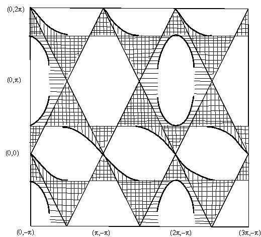
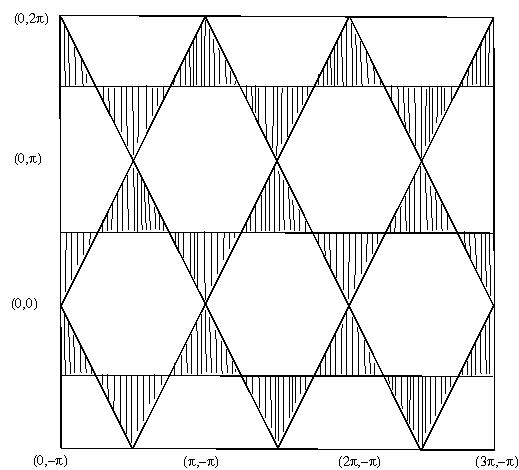
  Figure 10. Example (1): on the left the coamoeba when $\lambda\neq 0$ and the curve is non-Harnack, and the coamoeba when $\lambda=0$ and the triangulation is trivial on the right.

• Let $V_{f_{\lambda}}$ be the curve in $(\mathbb{C}^{*})^{2}$ defined by the following polynomial:

  $$f_{\lambda}(z,w)=zw^{2}+z^{2}w+z+w+\lambda zw.$$

  Let $f_{\lambda,\,1}(z,w)=zw^{2}+z+w+\lambda zw$. Hence $V_{f_{\lambda,\,1}}$ is just a reparametrization of the parabola of example 1. We can see that $z=-\frac{w}{1+w^{2}+\lambda w}$.
  Let $f_{\lambda,\,2}(z,w)=zw^{2}+z^{2}w+z+\lambda zw=z(1+zw+w^{2}+\lambda w)$, hence $V_{f_{\lambda,\,2}}$ is the set of points $(z,w)\in(\mathbb{C}^{*})^{2}$ such that :

  $$z=-\frac{1+w^{2}+\lambda w}{w}.$$

  It means that $\arg(z_{2})=-\arg(z_{1})$ mod $2\pi$, where $z_{1}$ (resp. $z_{2}$) denotes the first coordinate of a point in $V_{f_{\lambda,\,1}}$ (resp. in $V_{f_{\lambda,\,2}}$) . As in example 1, we have the figures 9 on the top right.

  

  

  

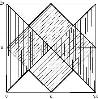
  Figure 11. Coamoeba of example (2) in three cases, the first coamoeba is the one of the Harnack case, the second coamoeba of a non-Harnack case and the coefficient $\lambda\neq 0$, and the last case is the case when $\lambda=0$ and the subdivision is trivial.

• We give an example of a Newton polygon $\Delta$ that defines not any real curve with maximal number of coamoeba complement components, but this maximal number is realized by a complex curve. Let $\Delta$ be the polygon with vertices $(1;0),\,(0;1),\,(1;2)$, and $(3;1)$ (see figure 10 for the polygon and its subdivision dual to the spine of the amoeba). In this case we prove that no real polynomial can realize the maximal number of coamoeba complement components (the maximal number in the real case is five, and the coamoeba is given in figure 11 on the left for some real coefficients ), but the complex curve defined by the complex polynomial $f(z,w)=e^{i\alpha}w+z+zw^{2}+z^{3}w$ with $0<\alpha<\pi$, has a coamoeba with maximal number of complement components (i.e. six components, see figure 11 on the right).

  

  

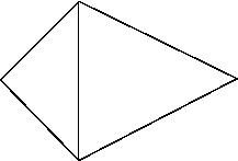
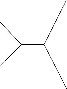
  Figure 12. The subdivision of the Newton polygon and its dual

  

  

  Figure 13. Example (3): on the left the coamoeba of a real curve with the same maximal number of complement components (i.e., 5 components; the picture here is in one fundamental domain) and on the right the coamoeba of a complex curve with a maximal number of complement components (6 components; the picture here is in four fundamental domains).

References

- [FPT-00] M. Forsberg, M; Passare and A. Tsikh, Laurent determinants and arrangements of hyperplane amoebas, Advances in Math. 151, (2000), 45-70.
- [GKZ-94] I. M. Gelfand, M. M. Kapranov and A. V. Zelevinski, Discriminants, resultants and multidimensional determinants, Birkhäuser Boston 1994.
- [IR-08] Z. Izhakian and L. Rowen, Completions, reversals, and duality for tropical varieties, http://fr.arxiv.org/pdf/0806.1175
- [IMS-07] I. Itenberg, G. Mikhalkin, and E. Shustin, Tropical Algebraic Geometry, Oberwolfach Seminars, Volume 35, Birkhäuser Basel-Boston-Berlin 2007.
- [K-00] M. M. Kapranov, Amoebas over non-Archimedean fields, Preprint 2000.
- [M1-02] G. Mikhalkin, Decomposition into pairs-of-pants for complex algebraic hypersurfaces,Topology 43, (2004), 1035-1065.
- [M2-04] G. Mikhalkin, Enumerative Tropical Algebraic Geometry In , J. Amer. Math. Soc. 18, (2005), 313-377.
- [M3-02] G. Mikhalkin , Real algebraic curves, moment map and amoebas, Ann.of Math. 151 (2000), 309-326.
- [N1-07] M. Nisse, Maximally sparse polynomials have solid amoebas, Preprint 2006, http://fr.arxiv.org/pdf/0704.2216
- [N2-07] M. Nisse, Coamoebas of complex algebraic hypersurfaces, Preprint, (2007).
- [N3-07] M. Nisse, Amoebas and Coamoebas Relations and Similarities, Preprint, (2007).
- [PR1-04] Passare and RullgårdM. Passare and H. Rullgård, Amoebas, Monge-Ampère measures, and triangulations of the Newton polytope, Duke Math. J. 121, (2004), 481-507.
- [PR2-01] M. Passare and H. Rullgård, Multiple Laurent series and polynomial amoebas, pp.123-130 in: Actes des rencontres d’analyse complexe, Atlantique, Éditions de l’actualité scientifique, Poitou-Charentes 2001.
- [PS-04] L. Pachter and B. Sturmfels, Algebraic Statistics for Computational Biology, Cambridge University Press, 2004.
- [RST-05] Richter-Gebert, Sturmfels, Theobald J. Richter-Gebert, B. Sturmfels et T. Theobald , First steps in tropical geometry, Idempotent mathematics and mathematical physics, Contemp. Math., 377, (2005), 289-317 , Amer. Math. Soc., Providence, RI, 2005.
- [R-01] H. Rullgård, Polynomial amoebas and convexity, Research Reports In Mathematics Number 8,2001, Department Of Mathematics Stockholm University.
- [V-90] O. Viro, Patchworking real algebraic varieties, preprint: http://www.math.uu.se/ oleg; Arxiv: AG/0611382