Modified Sonine approximation for granular binary mixtures

Abstract

We evaluate in this work the hydrodynamic transport coefficients of a granular binary mixture in $d$ dimensions. In order to eliminate the observed disagreement (for strong dissipation) between computer simulations and previously calculated theoretical transport coefficients for a monocomponent gas, we obtain explicit expressions of the seven Navier-Stokes transport coefficients with the use of a new Sonine approach in the Chapman-Enskog theory. Our new approach consists in replacing, where appropriate in the Chapman-Enskog procedure, the Maxwell-Boltzmann distribution weight function (used in the standard first Sonine approximation) by the homogeneous cooling state distribution for each species. The rationale for doing this lies in the fact that, as it is well known, the non-Maxwellian contributions to the distribution function of the granular mixture become more important in the range of strong dissipation we are interested in. The form of the transport coefficients is quite common in both standard and modified Sonine approximations, the distinction appearing in the explicit form of the different collision frequencies associated with the transport coefficients. Additionally, we numerically solve by means of the direct simulation Monte Carlo method the inelastic Boltzmann equation to get the diffusion and the shear viscosity coefficients for two and three dimensions. As in the case of a monocomponent gas, the modified Sonine approximation improves the estimates of the standard one, showing again the reliability of this method at strong values of dissipation.

1 Introduction

The success of the kinetic theory tools in describing granular gases has been widely recognized Goldhirsch (2003); Brilliantov & Pöschel (2004). In particular, the Navier-Stokes (NS) constitutive equations for the stress tensor and the heat flux of a monocomponent gas have been derived Sela & Goldhirsch (1998); Brey et al. (1998) by solving the inelastic Boltzmann equation by means of the Chapman-Enskog (CE) method to first order in the spatial gradients Chapman & Cowling (1970). As in the elastic case, the NS transport coefficients are given in terms of the solutions of linear integral equations Brey et al. (1998), which can be approximately solved to get the analytical dependence of these coefficients on dissipation. The standard method consists in approaching the solutions to these integral equations by the Maxwell-Boltzmann distribution $f_{M}$ times truncated Sonine polynomial expansions. For simplicity, usually only the lowest Sonine polynomial (first Sonine approximation) is retained (we will refer henceforth to this procedure as the standard Sonine approximation). In spite of this approximation, the results obtained from this approach (which formally applies for all values of the coefficient of restitution, see Brey et al., 1998) compare very well with Monte Carlo simulations Brey, Ruiz-Montero & Cubero (1999, 2000); Lutsko, Brey & Dufty (2002); Garzó & Montanero (2002) for mild degrees of inelasticity, namely, coefficients of restitution $\alpha$ that are larger than about 0.7. Specifically, while the self-diffusion and shear viscosity coefficients are well estimated by the first Sonine approximation (even for values of $\alpha$ smaller than 0.7), the transport coefficients associated with the heat flux present significant discrepancies with computer simulations Brey & Ruiz-Montero (2004); Brey et al. (2005a) for high dissipation ($\alpha\lesssim 0.7$). This fact has motivated the search for alternative methods which provide accurate estimates for the NS transport coefficients in the complete range of values of $\alpha$. Thus, Noskowicz et al. (2007) have used Borel resummation to obtain the distribution function of the homogeneous cooling state (HCS) and the NS transport coefficients. The method involves the solution of a system of algebraic equations that must be numerically solved. A different alternative consists in a slight modification of the Sonine polynomial approach, assuming that the isotropic part of the first order distribution function is mainly governed by the HCS distribution $f^{(0)}$ rather than by the Maxwellian distribution $f_{M}$ Lutsko (2005) (and this is what we call modified Sonine approximation). Except for this, this modified Sonine approximation keeps the usual structure of the standard Sonine approximation. Comparison with computer simulations Brey & Ruiz-Montero (2004); Brey, Ruiz-Montero, Maynar & García de Soria (2005a); Montanero, Santos & Garzó (2007) shows that this modified approximation significantly improves the accuracy of the NS transport coefficients of the single granular gas at strong dissipation Garzó, Santos & Montanero (2007c), especially in the case of the heat flux transport coefficients. The improved agreement in the range of high inelasticities is of physical relevance, since it helps to put into proper context the discussion vividly maintained in the field Aranson & Tsimring (2006); Goldhirsch (2003) about the existence (or not) of scale separation in granular gases. Moreover, the range of high inelasticities has growing interest in experimental works Clerc, Cordero, Dunstan, Huff, Mujica, Risso & Varas (2008); Vega Reyes & Urbach (2008a). Thus, it is important from a fundamental point of view to understand the origin of the discrepancies between theory and simulation for $\alpha\lesssim 0.7$.

Motivated by the good agreement found between theory and simulation for a monocomponent granular gas, we extend in this work the modified Sonine approach to the case of a granular binary mixture. Early attempts to obtain the NS transport coefficients were carried out by means of the CE expansion around Maxwellians at the same temperature for each species Jenkins & Mancini (1989); Zamankhan (1995); Arnarson & Willits (1998); Willits & Arnarson (1999); Serero, Goldhirsch, Noskowicz & Tan (2006). However, as confirmed by computer simulations Montanero & Garzó (2002); Barrat & Trizac (2002); Dahl, Hrenya, Garzó & Dufty (2002); Pagnani, Marconi & Puglisi (2002); Krouskop & Talbot (2003); Wang, Jin & Ma (2003); Brey, Ruiz-Montero & Moreno (2005b, 2006); Schröter, Ulrich, Kreft, Swift & Swinney (2006) and experiments Wildman & Parker (2002); Feitosa & Menon (2002), the equipartition assumption is not in general valid in granular mixtures since it is only close to being fulfilled in the quasielastic limit. A kinetic theory for granular mixtures at low density which accounts for nonequipartition effects has been developed in the past few years by Garzó & Dufty (2002). As in the single gas case, the above theory Garzó & Dufty (2002) shows that the NS transport coefficients of the mixture are given in terms of the solutions of a set of linear integral equations, which are approximately solved Garzó & Dufty (2002); Garzó, Montanero & Dufty (2006); Garzó & Montanero (2007) by means of the standard Sonine approximation. Furthermore, this theory has successfully predicted, as shown by computer simulations Montanero & Garzó (2002); Dahl, Hrenya, Garzó & Dufty (2002); Brey, Ruiz-Montero & Moreno (2005b); Schröter, Ulrich, Kreft, Swift & Swinney (2006), a constant ratio between the granular temperatures of both species. Here, we revisit the theory of Garzó & Dufty (2002) and solve the corresponding linear integral equations defining the NS transport coefficients by taking the HCS distribution $f_{i}^{(0)}$ ($i=1,2$) of each species as the weight function.

As expected, the problem for a binary mixture is much more involved than in the monocomponent case since not only the number of transport coefficients is larger but these coefficients are also functions of more parameters (masses, sizes, composition and three coefficients of restitution). In spite of these technical difficulties, explicit expressions for the seven relevant transport coefficients of the binary mixture (the mutual diffusion $D$, the pressure diffusion $D_{p}$, the thermal diffusion $D^{\prime}$, the shear viscosity $\eta$, the Dufour coefficient $D^{\prime\prime}$, the thermal conductivity $\lambda$, and the pressure energy coefficient $L$) have been obtained in terms of the parameter space of the problem. The results show that the modified Sonine approximation at large inelasticities introduces significant, moderate and slight corrections to the transport coefficients associated with the heat flux ($D^{\prime\prime}$, $\lambda$, $L$), stress tensor ($\eta$) and mass flux ($D$, $D_{p}$, $D^{\prime}$), respectively. In order to assess the degree of accuracy of the modified Sonine approximation, we have also performed Monte Carlo simulations for the mutual diffusion and the shear viscosity coefficients and use available simulation data for the heat flux coefficients in the monodisperse gas case Brey & Ruiz-Montero (2004); Brey, Ruiz-Montero, Maynar & García de Soria (2005a). We show that, in the range of strong inelasticity, the modified Sonine approximation provides better agreement with simulations in all cases, being this accuracy gain not negligible for viscosity, thermal conductivity, pressure energy coefficient and Duffour coefficient. This clearly justifies the use of this new approximation in order to obtain accurate expressions for the NS transport coefficients of the mixture.

An important issue is the applicability of the NS equations for granular binary mixtures derived here. The expressions of the seven NS transport coefficients are not restricted to weak inelasticity and hold for arbitrary values of the degree of dissipation. In fact, our modified Sonine approximation turns to be more accurate than the previous one Garzó & Dufty (2002) for very dissipative interactions. However, as already pointed out by Garzó et al. (2006), the NS hydrodynamic equations themselves may or may not be limited with respect to inelasticity, depending on the particular granular flows of real materials considered. It is important to recall that the CE method assumes that the relative changes of the hydrodynamic fields (partial densities, mean flow velocity and granular temperature) over distances of the order of the characteristic mean free path of the system are small. In the case of molecular or ordinary gas mixtures, the strength of the spatial gradients is controlled by external sources (the initial or boundary conditions, driving forces), and for a great variety of experimental conditions of practical interest the NS hydrodynamic equations describe adequately the hydrodynamics of the system. Unfortunately, the situation in the case of granular gases is more complex, since in most problems of practical interest (such as steady states) the boundary conditions cannot completely control by themselves the spatial gradients of the hydrodynamic fields. This is due to collisional cooling, which sets a minimum value for the relative size of the steady state gradients. An example of this situation corresponds to the well-known (steady) simple shear flow state Goldhirsch (2003); Santos, Garzó & Dufty (2004). This type of flow can only occur when collisional cooling (which is fixed by the mechanical properties of the particles making up the fluid) is exactly balanced by viscous heating. Unfortunately, this occurs, except for the quasielastic limit, only for very extreme boundary conditions (high shear). The same applies for all steady states for a granular gas heated or sheared from the boundaries, although the behaviour of the gradients is qualitatively different for each type of flow (for a case by case study, please refer to the work by Vega Reyes & Urbach, 2008b). Another example is the case of a granular gas bounded by two opposite walls at rest and at the same temperature. Recent comparisons Hrenya, Galvin & Wildman (2008) between molecular dynamics simulations and kinetic theory provide evidence that higher-order effects (i.e., beyond the NS description) can be measurable for moderate inelasticities.

Nevertheless, in spite of the above cautions, the NS description is still accurate and appropriate for a wide class of flows. One of them corresponds to small spatial perturbations of the homogeneous cooling state for an isolated system Brey, Dufty, Santos & Kim (1998); Garzó (2005). Both molecular dynamics and Monte Carlo simulations Brey, Ruiz-Montero & Cubero (1999, 2000) have quantitatively confirmed the dependence of the NS transport coefficients on dissipation (even for strong values of the coefficient of restitution) and the applicability of the NS hydrodynamics with these transport coefficients to describe cluster formation. Another interesting example consists of the application of the NS hydrodynamics from kinetic theory to characterize the symmetry breaking as well as the density and temperature profiles in vertical vibrated gases Brey, Ruiz-Montero, Moreno & García-Rojo (2002). In the case of dense gases, there is evidence of the good agreement found between the NS coefficients derived from the Enskog kinetic theory Garzó & Dufty (1999a) and computer simulations Lutsko, Brey & Dufty (2002); Dahl, Hrenya, Garzó & Dufty (2002); Lois, Lemaître & Carlson (2007). Similar comparisons between NS hydrodynamics and real experiments of supersonic flow past a wedge Rericha, Bizon, Shattuck & Swinney (2002) and Nuclear Magnetic Resonance (NMR) experiments of a system of mustard seeds vibrated vertically Yang, Huan, Candela, Mair & Walsworth (2002); Huan, Yang, Candela, Mair & Walsworth (2004) have shown both qualitative and quantitative agreement. Furthermore, the Navier-Stokes hydrodynamics accounts for a variety of properties of granular flows that are preserved beyond NS order. For instance, the curvature of the temperature profile: the same types of steady profiles predicted by NS hydrodynamics have been observed in DSMC simulations beyond the NS domain, as it is reported in a recent theoretical work where new steady states (exclusive to granular gases) have been found Vega Reyes & Urbach (2008b). Therefore, the NS equations with the transport coefficients derived here can be considered still as an useful theory for a wide class of rapid granular flows, although more limited than for ordinary gases.

The plan of the paper is as follows. In § 2, the full transport coefficients of the mixture are given in terms of the solutions of a set of coupled linear integral equations previously derived by Garzó & Dufty (2002). These integral equations are approximately solved by means of the modified first Sonine approximation in § 3 where explicit forms for the transport coefficients are provided. Technical details of the calculations carried out here are given in two Appendices and in a Supplementary Material submitted in the online version of the paper. Next, in § 4 the results obtained for these seven transport coefficients from the standard and modified Sonine approximations are compared for several cases. In addition, both theoretical approaches are also compared with available and new simulation data obtained from numerical solutions of the Boltzmann equation by using the direct simulation Monte Carlo (DSMC) method Bird (1994) in the cases of the diffusion and shear viscosity coefficients, both for two- and three-dimensional systems. The paper is closed in § 5 with a discussion of the results presented in this paper.

2 Navier-Stokes transport coefficients for a granular binary mixture

We consider a binary mixture composed by smooth inelastic disks ($d=2$) or spheres ($d=3$) of masses $m_{1}$ and $m_{2}$, and diameters $\sigma_{1}$ and $\sigma_{2}$. The inelasticity of collisions among all pairs is characterized by three independent constant coefficients of restitution $\alpha_{11}$, $\alpha_{22}$, and $\alpha_{12}=\alpha_{21}$, where $\alpha_{ij}\leq 1$ is the coefficient of restitution for collisions between particles of species $i$ and $j$. In the low-density regime, the one-particle velocity distribution functions $f_{i}({\boldsymbol{r}},{\boldsymbol{v}},t)$ obey the set of (inelastic) Boltzmann equations Goldshtein & Shapiro (1995); Brey, Dufty & Santos (1997). When the hydrodynamic gradients present in the system are weak, the CE method Chapman & Cowling (1970) conveniently adapted to dissipative dynamics provides a solution to the Boltzmann equation based on an expansion

$$f_{i}=f_{i}^{(0)}+f_{i}^{(1)}+\cdots,$$ (1)

where $f_{i}^{(0)}$ is the local version of the homogeneous cooling state (HCS) Garzó & Dufty (1999b). Although the exact form of the distribution $f_{i}^{(0)}$ is not known (even in the one-component case), an indirect information of the behavior of $f_{i}^{(0)}$ is given through its velocity moments. In particular, the deviation of $f_{i}^{(0)}$ from its Maxwellian form can be characterized by the fourth cumulant

$$c_{i}=2\left[\frac{m_{i}^{2}}{n_{i}T_{i}^{2}}\frac{1}{d(d+2)}\int\;d{\boldsymbol{v}}\;V^{4}f_{i}^{(0)}-1\right],$$ (2)

where ${\boldsymbol{V}}={\boldsymbol{v}}-{\boldsymbol{U}}$ is the peculiar velocity,

$$n_{i}=\int\;d{\boldsymbol{v}}\;f_{i}^{(0)}$$ (3)

is the number density of species $i$,

$${\boldsymbol{U}}=\frac{1}{\rho}\sum_{i=1}^{2}\;\int\;d{\boldsymbol{v}}\;m_{i}{\bf v}\;f_{i}^{(0)}$$ (4)

is the mean flow velocity and $\rho=m_{1}n_{1}+m_{2}n_{2}$ is the total mass density.

The first-order distribution $f_{i}^{(1)}$ has the form Garzó & Dufty (2002)

$$f_{i}^{(1)}={\boldsymbol{\cal A}}_{i}\boldsymbol{\cdot}\boldsymbol{\nabla}x_{1}+{\boldsymbol{\cal B}}_{i}\boldsymbol{\cdot}\boldsymbol{\nabla}p+{\boldsymbol{\cal C}}_{i}\boldsymbol{\cdot}\boldsymbol{\nabla}T+{\cal D}_{i,k\ell}\boldsymbol{\nabla}_{k}U_{\ell}\;,$$ (5)

where $x_{i}=n_{i}/n$ is the mole fraction of species $i$,

$$T=\frac{1}{dn}\sum_{i=1}^{2}\;\int\;d{\boldsymbol{v}}\;m_{i}V^{2}\;f_{i}^{(0)}$$ (6)

is the temperature and $p=nT$ is the pressure. Here, $n=\sum_{i}n_{i}$ is the total number density. The coefficients ${\boldsymbol{\cal A}}_{i}$, ${\boldsymbol{\cal B}}_{i}$, ${\boldsymbol{\cal C}}_{i}$, and ${\mathsfbi{\cal D}}_{i}$ are functions of the peculiar velocity ${\boldsymbol{V}}={\boldsymbol{v}}-{\boldsymbol{U}}$ and the hydrodynamic fields.

The knowledge of the distributions $f_{i}^{(1)}$ allows us to determine the NS transport coefficients. The analysis to obtain them has been previously worked out by Garzó and coworkers Garzó & Dufty (2002); Garzó et al. (2006); Garzó & Montanero (2007). For the sake of completeness, the final results will be displayed in this Section. The mass flux ${\bf j}_{1}^{(1)}$, the pressure tensor $P_{k\ell}^{(1)}$, and the heat flux ${\bf q}^{(1)}$ are given, respectively, by Garzó & Dufty (2002)

$${\boldsymbol{j}}_{1}^{(1)}=-\frac{m_{1}m_{2}n}{\rho}D\boldsymbol{\nabla}x_{1}-\frac{\rho}{p}D_{p}\boldsymbol{\nabla}p-\frac{\rho}{T}D^{\prime}\boldsymbol{\nabla}T,\hskip 21.68121pt{\boldsymbol{j}}_{2}^{(1)}=-{\boldsymbol{j}}_{1}^{(1)},$$ (7)

$$\mathsfbi{P}_{k\ell}^{(1)}=p\;\delta_{k\ell}-\eta\left(\boldsymbol{\nabla}_{\ell}U_{k}+\boldsymbol{\nabla}_{k}U_{\ell}-\frac{2}{d}\delta_{k\ell}{\boldsymbol{\nabla}\boldsymbol{\cdot}U}\right),$$ (8)

$${\boldsymbol{q}}^{(1)}=-T^{2}D^{\prime\prime}\boldsymbol{\nabla}x_{1}-L\boldsymbol{\nabla}p-\lambda\boldsymbol{\nabla}T.$$ (9)

It must be noted that the contribution to first order in the gradients of the collisional cooling vanishes ($\zeta^{(1)}=0$) by symmetry and there is no need to consider here this term Brey et al. (1998). This is due to the fact that the cooling rate is a scalar and so, corrections to first order in gradients can arise only from the divergence of the velocity field. However, as Eq. (5) shows, there is no contribution to $f_{i}^{(1)}$ proportional to $\nabla\cdot{\bf U}$ and consequently, $\zeta^{(1)}=0$. This is special to the low density Boltzmann equation and such terms occur at higher densities Garzó & Dufty (1999a); Garzó et al. (2007b).

The transport coefficients appearing in (7)–(9) are the diffusion coefficient $D$, the pressure diffusion coefficient $D_{p}$, the thermal diffusion coefficient $D^{\prime}$, the shear viscosity $\eta$, the Dufour coefficient $D^{\prime\prime}$, the pressure energy coefficient $L$, and the thermal conductivity $\lambda$. These coefficients are defined as

$$D=-\frac{\rho}{dm_{2}n}\int d{\boldsymbol{v}}\,{\boldsymbol{V}}\boldsymbol{\cdot}{\boldsymbol{\cal A}}_{1},$$ (10)

$$D_{p}=-\frac{m_{1}p}{d\rho}\int d{\boldsymbol{v}}\,{\boldsymbol{V}}\boldsymbol{\cdot}{\boldsymbol{\cal B}}_{1},$$ (11)

$$D^{\prime}=-\frac{m_{1}T}{d\rho}\int d{\boldsymbol{v}}\,{\boldsymbol{V}}\boldsymbol{\cdot}{\boldsymbol{\cal C}}_{1},$$ (12)

$$\eta=-\frac{1}{(d-1)(d+2)}\sum_{i=1}^{2}\,m_{i}\,\int d{\boldsymbol{v}}\,{\boldsymbol{V}}{\boldsymbol{V}}:{{\cal D}}_{i},$$ (13)

$$D^{\prime\prime}=-\frac{1}{dT^{2}}\sum_{i=1}^{2}\,\frac{m_{i}}{2}\,\int d{\boldsymbol{v}}\,V^{2}{\boldsymbol{V}}\boldsymbol{\cdot}{\boldsymbol{\cal A}}_{i},$$ (14)

$$L=-\frac{1}{d}\sum_{i=1}^{2}\,\frac{m_{i}}{2}\,\int d{\boldsymbol{v}}\,V^{2}{\boldsymbol{V}}\boldsymbol{\cdot}\,{\boldsymbol{\cal B}}_{i},$$ (15)

$$\lambda=-\frac{1}{d}\sum_{i=1}^{2}\,\frac{m_{i}}{2}\,\int d{\boldsymbol{v}}\,V^{2}{\boldsymbol{V}}\boldsymbol{\cdot}{\boldsymbol{\cal C}}_{i}.$$ (16)

As in the case of elastic collisions Chapman & Cowling (1970), the unknowns are the solutions of a set of coupled linear integral equations. Their explicit forms are given in the Supplementary Material file of this article and by Eqs. (46)–(49) of Garzó & Dufty (2002).

3 Modified First Sonine approximation

The results presented in the above Section are still exact. However, to get the explicit dependence of the NS transport coefficients on the parameters of the mixture (masses, sizes, composition, coefficients of restitution), one has to solve the integral equations obeying ${\boldsymbol{\cal A}}_{i}$, ${{\cal B}}_{i}$, ${\boldsymbol{\cal C}}_{i}$, and ${\boldsymbol{\cal D}}_{i}$ as well as one has to know the explicit forms of $f_{i}^{(0)}$ and of the HCS cooling rate $\zeta^{(0)}$ (see Appendix A and the work by Garzó & Dufty (1999b) for more details). With respect to the distribution $f_{i}^{(0)}$, except in the high velocity region, it is very accurately estimated by Garzó & Dufty (1999b); Montanero & Garzó (2002)

$$f_{i}^{(0)}({\boldsymbol{V}})=f_{i,M}({\boldsymbol{V}})\left[1+\frac{c_{i}}{4}\left(\theta_{i}^{2}V^{*4}-(d+2)\theta_{i}V^{*2}+\frac{d(d+2)}{4}\right)\right],$$ (17)

where $c_{i}$ is defined by (2), $V^{*}=V/v_{0}$, $\theta_{i}=m_{i}\gamma_{i}^{-1}\sum_{j}m_{j}^{-1}$, and

$$v_{0}=\sqrt{\frac{2T(m_{1}+m_{2})}{m_{1}m_{2}}}$$ (18)

is a thermal speed. Further, $\gamma_{i}=T_{i}/T$ is the temperature ratio and $f_{i,M}$ is the Maxwellian distribution

$$f_{i,M}({\boldsymbol{V}})=n_{i}\left(\frac{m_{i}}{2\pi T_{i}}\right)^{d/2}\exp\left(-\frac{m_{i}V^{2}}{2T_{i}}\right).$$ (19)

The partial temperatures $T_{i}$ are defined as

$$T_{i}=\frac{1}{dn_{i}}\int\;d{\boldsymbol{v}}\;m_{i}V^{2}\;f_{i}^{(0)}.$$ (20)

The cumulant $c_{i}$ measures the departure of $f_{i}^{(0)}$ from $f_{i,M}$. The temperature ratios $\gamma_{i}$ along with the coefficients $c_{i}$ and the cooling rate $\zeta^{(0)}$ have been determined for inelastic hard spheres ($d=3$) Garzó & Dufty (1999b). These calculations have been extended here in § Appendix A to an arbitrary number of dimensions.

With respect to the functions $\left\{{\boldsymbol{\cal A}}_{i},{\boldsymbol{\cal B}}_{i},{\boldsymbol{\cal C}}_{i},{{\cal D}}_{i}\right\}$, as in the elastic case, the simplest approximation consists of expanding them in a series of Sonine polynomials and consider only the leading terms in this expansion. Usually, for simplicity, the polynomials are defined with respect to a Gaussian weight factor. This alternative has been previously used Garzó & Dufty (2002); Garzó & Montanero (2007) to get explicit forms for the NS transport coefficients. The accuracy of these theoretical predictions (based on the standard first Sonine approximation) over a wide range of inelasticities has been confirmed by Monte Carlo simulations of the Boltzmann equation in the cases of the tracer diffusion coefficient Garzó & Montanero (2007, 2004) and the shear viscosity coefficient Garzó & Montanero (2007); Montanero & Garzó (2003). However, as said in the Introduction, recent comparisons with computer simulations for the transport coefficients associated with the heat flux for a monocomponent gas have shown significant discrepancies for strong inelasticities Brey & Ruiz-Montero (2004); Brey et al. (2005a); Montanero et al. (2007). This fact has motivated the search for new approaches, such as a modified first Sonine approximation Garzó et al. (2007c).

As already pointed out by Garzó et al. (2007c), one of the possible sources of discrepancy between the standard first Sonine approximation and computer simulations for the heat flux transport coefficients could be the emergence of the existing non-Gaussian features of the zeroth-order distribution function $f_{i}^{(0)}$. Although the Maxwellian distribution $f_{i,M}$ is a good approximation to $f_{i}^{(0)}$ in the region of thermal velocities relevant to low degree velocity moments (hydrodynamic quantities, mass flux), quantitative discrepancies between $f_{i,M}$ and $f_{i}^{(0)}$ are expected to be important when one evaluates higher degree velocity moments, such as the pressure tensor and the heat flux, specially for strong dissipation. However, the behavior of the first-order distribution $f_{i}^{(1)}$ in the standard Sonine approximation Garzó & Dufty (2002) is mainly governed by the Maxwellian distribution $f_{i,M}$ and not by the HCS distribution $f_{i}^{(0)}$. A possible way of mitigating the discrepancies between the standard first Sonine approximation and simulations would be to incorporate more terms in the Sonine polynomial expansion Garzó & Montanero (2004), but the technical difficulties to evaluate these new contributions for general binary mixtures discard this method. Here, we follow the same route as in our previous work Garzó et al. (2007c) for monocomponent gases and take the distribution $f_{i}^{(0)}$ instead of the simple Maxwellian form $f_{i,M}$ as the convenient weight function. In this case, some care must be taken in the structure of the velocity polynomials chosen to preserve the solubility conditions of the CE method Chapman & Cowling (1970); Garzó & Santos (2003). These conditions are given by

$$\int d{\boldsymbol{v}}f_{i}^{(1)}({\boldsymbol{v}})=0\;,\$$ (21)

$$\sum_{i=1}^{2}\,m_{i}\,\int d{\boldsymbol{v}}\,{\boldsymbol{v}}f_{i}^{(1)}({\boldsymbol{v}})={\boldsymbol{0}}\;,$$ (22)

$$\sum_{i=1}^{2}\,\frac{m_{i}}{2}\,\int d{\boldsymbol{v}}\,V^{2}f_{i}^{(1)}({\boldsymbol{v}})=0\;.$$ (23)

While the conditions (21) and (22) yield the same velocity polynomials as in the standard method, in order to preserve the solubility condition (23) one has to replace the polynomial

$${\boldsymbol{S}}_{i}({\boldsymbol{V}})=\left(\frac{1}{2}m_{i}V^{2}-\frac{d+2}{2}T_{i}\right){\bf V}$$ (24)

appearing in the standard Sonine polynomial expansion Garzó & Dufty (2002) by the modified polynomial

$${\overline{\boldsymbol{S}}}_{i}({\boldsymbol{V}}) = \left(\frac{1}{2}m_{i}V^{2}-\frac{d+2}{2}\left(1+\frac{1}{2}c_{i}\right)T_{i}\right){\bf V}$$ (25)

$$= {\boldsymbol{S}}_{i}({\boldsymbol{V}})-\frac{d+2}{4}c_{i}T_{i}{\bf V}.$$

As will be shown later, this replacement gives rise to new contributions to the transport coefficients associated with the heat flux.

The determination of the NS transport coefficients in the modified first Sonine approximation follows similar mathematical steps as the ones previously used in the standard first Sonine approximation. More specific technical details on these calculations are available as a supplement to the online version of this paper or on request from the authors. Here, we only display the final expressions for the NS transport coefficients in terms of the parameter space of the problem.

3.1 Mass flux transport coefficients

The mass flux contains three transport coefficients: $D$, $D_{p}$, and $D^{\prime}$. Dimensionless forms are defined by

$$D=\frac{\rho T}{m_{1}m_{2}\nu_{0}}D^{*},\quad D_{p}=\frac{p}{\rho\nu_{0}}D_{p}^{*},\quad D^{\prime}=\frac{p}{\rho\nu_{0}}D^{{}^{\prime}*}$$ (26)

where $\nu_{0}=n\sigma_{12}^{d-1}v_{0}$ is an effective collision frequency and $\sigma_{12}=(\sigma_{1}+\sigma_{2})/2$. The explicit forms are then

$$D^{*}=\left(\nu_{D}-\frac{1}{2}\zeta^{\ast}\right)^{-1}\left[\left(\frac{\partial}{\partial x_{1}}x_{1}\gamma_{1}\right)_{p,T}+\left(\frac{\partial\zeta^{\ast}}{\partial x_{1}}\right)_{p,T}\left(1-\frac{\zeta^{\ast}}{2\nu_{D}}\right)D_{p}\right],$$ (27)

$$D_{p}^{*}=x_{1}\left(\gamma_{1}-\frac{\mu}{x_{2}+\mu x_{1}}\right)\left(\nu_{D}-\frac{3}{2}\zeta^{\ast}+\frac{\zeta^{\ast 2}}{2\nu_{D}}\right)^{-1},$$ (28)

$$D^{\prime*}=-\frac{\zeta^{\ast}}{2\nu_{D}}D_{p}^{*}.$$ (29)

In these equations, $\zeta^{*}=\zeta^{(0)}/\nu_{0}$, $\mu=m_{1}/m_{2}$ is the mass ratio and the expression of $\nu_{D}$ is given by Eq. (51) of the Appendix B .

3.2 Shear viscosity coefficient

The shear viscosity coefficient $\eta$ is given by

$$\eta=\frac{p}{\nu_{0}}\left(x_{1}T_{1}^{2}\eta_{1}^{*}+x_{2}T_{2}^{2}\eta_{2}^{*}\right),$$ (30)

where the partial contributions $\eta_{i}^{*}$ to the shear viscosity are

$$\eta_{1}^{*}=\frac{2\gamma_{2}(2\tau_{22}-\zeta^{*})-4\gamma_{1}\tau_{12}}{\gamma_{1}\gamma_{2}[\zeta^{*2}-2\zeta^{*}(\tau_{11}+\tau_{22})+4(\tau_{11}\tau_{22}-\tau_{12}\tau_{21})]},$$ (31a)

$$\eta_{2}^{*}=\frac{2\gamma_{1}(2\tau_{11}-\zeta^{*})-4\gamma_{2}\tau_{21}}{\gamma_{1}\gamma_{2}[\zeta^{*2}-2\zeta^{*}(\tau_{11}+\tau_{22})+4(\tau_{11}\tau_{22}-\tau_{12}\tau_{21})]},$$ (31b)

where the collision frequencies $\tau_{ij}$ are given by Eqs. (53)–(56).

3.3 Heat flux transport coefficients

The transport coefficients $D^{\prime\prime}$, $L$, and $\lambda$ associated with the heat flux can be written as

$$D^{\prime\prime}=-\frac{d+2}{2}\frac{n}{(m_{1}+m_{2})\nu_{0}}\left[\frac{x_{1}\gamma_{1}^{3}}{\mu_{12}}d_{1}^{*}+\frac{x_{2}\gamma_{2}^{3}}{\mu_{21}}d_{2}^{*}-\left(\frac{\gamma_{1}}{\mu_{12}}-\frac{\gamma_{2}}{\mu_{21}}\right)D^{\ast}\right],$$ (32)

$$L=-\frac{d+2}{2}\frac{T}{(m_{1}+m_{2})\nu_{0}}\left[\frac{x_{1}\gamma_{1}^{3}}{\mu_{12}}\ell_{1}^{*}+\frac{x_{2}\gamma_{2}^{3}}{\mu_{21}}\ell_{2}^{*}-\left(\frac{\gamma_{1}}{\mu_{12}}-\frac{\gamma_{2}}{\mu_{21}}\right)D_{p}^{\ast}\right],$$ (33)

$$\lambda=-\frac{d+2}{2}\frac{nT}{(m_{1}+m_{2})\nu_{0}}\left[\frac{x_{1}\gamma_{1}^{3}}{\mu_{12}}\lambda_{1}^{*}+\frac{x_{2}\gamma_{2}^{3}}{\mu_{21}}\lambda_{2}^{*}-\left(\frac{\gamma_{1}}{\mu_{12}}-\frac{\gamma_{2}}{\mu_{21}}\right)D^{\prime}{}^{\ast}\right],$$ (34)

where $\mu_{ij}=m_{i}/(m_{i}+m_{j})$ and the coefficients $D^{\ast}$, $D_{p}^{\ast}$, and $D^{\prime\ast}$ are given by Eqs. (27)–(29), respectively. The expressions of the (dimensionless) coefficients $d_{i}^{*}$, $\ell_{i}^{*}$, and $\lambda_{i}^{*}$ are

$$d_{1}^{*} = \frac{1}{\Lambda}\left\{2\left[2\nu_{12}Y_{2}-Y_{1}(2\nu_{22}-3\zeta^{*})\right]\left[\nu_{12}\nu_{21}-\nu_{11}\nu_{22}+2(\nu_{11}+\nu_{22})\zeta^{*}-4\zeta^{*2}\right]\right.$$ (35)

$$+2\left(\frac{\partial\zeta^{\ast}}{\partial x_{1}}\right)_{p,T}(Y_{3}+Y_{5})\left[2\nu_{12}\nu_{21}+2\nu_{22}^{2}-\zeta^{*}(7\nu_{22}-6\zeta^{*})\right]$$

$$\left.-2\nu_{12}\left(\frac{\partial\zeta^{\ast}}{\partial x_{1}}\right)_{p,T}(Y_{4}+Y_{6})\left(2\nu_{11}+2\nu_{22}-7\zeta^{*}\right)\right\},$$

$$\ell_{1}^{*} = \frac{1}{\Lambda}\left\{-2Y_{3}\left[2(\nu_{12}\nu_{21}-\nu_{11}\nu_{22})\nu_{22}+\zeta^{*}(7\nu_{11}\nu_{22}-5\nu_{12}\nu_{21}+2\nu_{22}^{2}\right.\right.$$ (36)

$$\left.-6\nu_{11}\zeta^{*}-7\nu_{22}\zeta^{*}+6\zeta^{*2})\right]+2Y_{4}\nu_{12}\left[2\nu_{12}\nu_{21}-2\nu_{11}\nu_{22}+2\zeta^{*}(\nu_{11}+\nu_{22})-\zeta^{*2}\right]$$

$$+ \left.2Y_{5}\zeta^{*}\left[2\nu_{12}\nu_{21}+\nu_{22}(2\nu_{22}-7\zeta^{*})+6\zeta^{*2}\right]-2\nu_{12}\zeta^{*}Y_{6}\left[2(\nu_{11}+\nu_{22})-7\zeta^{*}\right]\right\},$$

$$\lambda_{1}^{*} = \frac{1}{\Lambda}\left\{-Y_{3}\zeta^{*}\left[2\nu_{12}\nu_{21}+\nu_{22}(2\nu_{22}-7\zeta^{*})+6\zeta^{*2}\right]+\nu_{12}\zeta^{*}Y_{4}\left[2(\nu_{11}+\nu_{22})-7\zeta^{*}\right]\right.$$ (37)

$$-Y_{5}\left[4\nu_{12}\nu_{21}(\nu_{22}-\zeta^{*})+2\nu_{22}^{2}(5\zeta^{*}-2\nu_{11})+2\nu_{11}(7\nu_{22}\zeta^{*}-6\zeta^{*2})+5\zeta^{*2}(6\zeta^{*}-7\nu_{22})\right]$$

$$\left.+\nu_{12}Y_{6}\left[4\nu_{12}\nu_{21}+2\nu_{11}(5\zeta^{*}-2\nu_{22})+\zeta^{*}(10\nu_{22}-23\zeta^{*})\right]\right\}.$$

Here, the Y’s are defined by (57)–(62),

$$\Lambda=\left[4(\nu_{12}\nu_{21}-\nu_{11}\nu_{22})+6\zeta^{*}(\nu_{11}+\nu_{22})-9\zeta^{*2}\right]\left[\nu_{12}\nu_{21}-\nu_{11}\nu_{22}+2\zeta^{*}(\nu_{11}+\nu_{22})-4\zeta^{*2}\right],$$ (38)

and the (reduced) collision frequencies $\nu_{ij}$ are given by Eqs. (B) and (B). The corresponding expressions for $d_{2}^{\prime\prime}$, $\ell_{2}$, $\lambda_{2}$, $\nu_{22}$, and $\nu_{21}$ can be deduced from (35)–(37) by interchanging $1\leftrightarrow 2$. With these results, the coefficients $D^{\prime\prime}$, $L$, and $\lambda$ can be explicitly obtained from (32)–(34). In (35)–(37) it is understood that the coefficients $D^{*}$, $D_{p}^{*}$, and $D^{{}^{\prime}*}$ are given by (27)–(29), respectively. Of course, our results show that $D^{{}^{\prime\prime}}$ is antisymmetric with respect to the change $1\leftrightarrow 2$ while $L$ and $\lambda$ are symmetric. Consequently, in the case of mechanically equivalent particles ($m_{1}=m_{2}$, $\sigma_{1}=\sigma_{2}$, $\alpha_{ij}=\alpha$), the coefficient $D^{{}^{\prime\prime}}=0$.

The expressions for the NS transport coefficients derived here for a granular binary mixture reduce to those previously obtained Garzó & Montanero (2007) when one takes Maxwellians distributions for the reference homogeneous cooling state $f_{i}^{(0)}$ ($c_{1}=c_{2}=0$). In addition, for mechanically equivalent particles, the results obtained by Garzó et al. (2007c) for a single gas by using the modified Sonine method are also recovered. This confirms the self-consistency of the results reported in this paper.

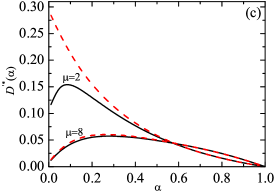
Figure 1: Plot of the reduced coefficients $D(\alpha)/D(1)$ (a), $D_{p}(\alpha)/D_{p}(1)$ (b), and $D^{{}^{\prime}*}(\alpha)$ (c) as functions of the coefficient of restitution $\alpha$ for hard spheres with $x_{1}=\frac{1}{2}$, $\sigma_{1}=\sigma_{2}$ and two different values of the mass ratio $\mu=m_{1}/m_{2}$. The solid lines correspond to the results obtained from the modified first Sonine approximation while the dashed lines refer to the results obtained from the standard first Sonine approximation.

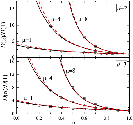
Figure 2: Plot of the reduced diffusion coefficient $D(\alpha)/D(1)$ as a function of the coefficient of restitution $\alpha$ for hard disks (top panel) and hard spheres (bottom panel) in the tracer limit ($x_{1}\to 0)$ when the tagged particle has the same mass density as the particles of the gas ($\mu=\omega^{d}$). Three different values of the mass ratio have been considered: $\mu=1$, $\mu=4$ and $\mu=8$. The solid and dashed lines represent the modified and standard first Sonine approximations, respectively. The symbols are DSMC results obtained from the mean square displacement of the tagged particle. The DSMC results correspond to $\mu=1$ (circles), $\mu=4$ (triangles), and $\mu=8$ (squares).

4 Comparison with the standard first Sonine approximation and with Monte Carlo simulations

The expressions for the transport coefficients derived in the previous Section depend on many parameters: $\{x_{1},m_{1}/m_{2},\sigma_{1}/\sigma_{2},\alpha_{11},\alpha_{22},\alpha_{12}\}$. Obviously, this complexity exists in the elastic limit as well, so that the primary new feature is the dependence of the transport coefficients on dissipation. Thus, to show more clearly the influence of inelasticity in collisions on transport, we normalize the transport coefficients with respect to their values in the elastic limit. Also, for simplicity, we take the simplest case of common coefficient of restitution ($\alpha_{11}=\alpha_{22}=\alpha_{12}\equiv\alpha$). This reduces the parameter space to four quantities: $\{x_{1},m_{1}/m_{2},\sigma_{1}/\sigma_{2},\alpha\}$.

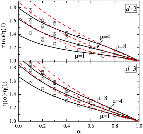
Figure 3: Plot of the reduced shear viscosity coefficient $\eta(\alpha)/\eta(1)$ as a function of the coefficient of restitution $\alpha$ for hard disks (top panel) and hard spheres (bottom panel) for an equimolar mixture ($x_{1}=\frac{1}{2})$ constituted by particles of the same mass density ($\mu=\omega^{d}$). Three different values of the mass ratio have been considered: $\mu=1$, $\mu=4$ and $\mu=8$. The solid and dashed lines represent the modified and standard first Sonine approximations, respectively. The DSMC results correspond to $\mu=1$ (circles), $\mu=4$ (triangles), and $\mu=8$ (squares).

Let us start with the coefficients $D$, $D_{p}$ and $D^{\prime}$ associated with the mass flux. In Fig. 1 the reduced coefficients $D(\alpha)/D(1)$, $D_{p}(\alpha)/D_{p}(1)$ and $D^{{}^{\prime}*}$, defined by (29), are plotted as functions of the coefficient of restitution $\alpha$ for an equimolar mixture $x_{1}=\frac{1}{2}$ of hard spheres ($d=3$) with the same size ratio $\omega\equiv\sigma_{1}/\sigma_{2}=1$ and three different values of the mass ratio $\mu\equiv m_{1}/m_{2}$. Here, $D(1)$ and $D_{p}(1)$ refer to the elastic values of $D$ and $D_{p}$, respectively. The coefficient $D^{{}^{\prime}}$ has not been reduced with respect to its elastic value since $D^{\prime}=0$ for $\alpha=1$. We observe that both Sonine approximations lead to quite identical results, except for quite extreme values of dissipation where both approaches present some discrepancies. This is especially important in the case $\mu=2$ where the disagreement is, for instance, about 15% and 32% for the coefficient $D_{p}$ at $\alpha=0.1$ and 0.2, respectively. In order to test the accuracy of both Sonine approximations in the case of the diffusion coefficients, the dependence of the (reduced) diffusion coefficient $D(\alpha)/D(1)$ on $\alpha$ is plotted in Fig. 2 in the tracer limit ($x_{1}\to 0$) for two different cases when the tagged particle has the same mass density as the particles of the gas (i.e., $\mu=\omega^{d}$). The theoretical predictions of both Sonine approximations are compared with available Garzó & Montanero (2004, 2007) and new Monte Carlo simulations (using the DSMC method, Bird, 1994). Here, the tracer diffusion coefficient has been measured in computer simulations from the mean square displacement of a tagged particle in the HCS Garzó & Montanero (2004). It is apparent that both Sonine approximations provide a general good agrement with simulation data. However, the standard approximation slightly overestimates the diffusion coefficient at high inelasticity, this effect being corrected by the modified approximation.

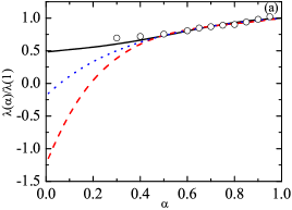
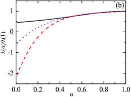
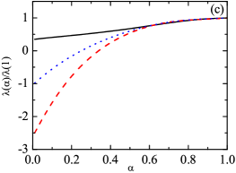
Figure 4: Plot of the reduced thermal conductivity coefficient $\lambda(\alpha)/\lambda(1)$ for hard spheres with $x_{1}=\frac{1}{2}$, $\sigma_{1}=\sigma_{2}$ and three different values of the mass ratio $\mu$: $\mu=1$ (a), $\mu=2$ (b), and $\mu=8$ (c). The solid lines correspond to the results obtained from the modified first Sonine approximation, the dashed lines refer to the results obtained from the standard first Sonine approximation while the dotted lines are the results derived by neglecting non-Gaussian corrections to the HCS distributions. The symbols in the panel (a) are DSMC results obtained from the Green-Kubo relations for a monocomponent gas Brey & Ruiz-Montero (2004).

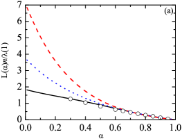
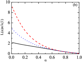
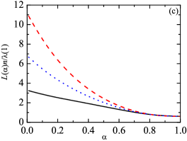
Figure 5: Plot of the reduced pressure energy coefficient $L(\alpha)n/\lambda(1)$ for hard spheres with $x_{1}=\frac{1}{2}$, $\sigma_{1}=\sigma_{2}$ and three different values of the mass ratio $\mu$: $\mu=1$ (a), $\mu=2$ (b), and $\mu=8$ (c). The solid lines correspond to the results obtained from the modified first Sonine approximation, the dashed lines refer to the results obtained from the standard first Sonine approximation while the dotted lines are the results derived by neglecting non-Gaussian corrections to the HCS distributions. The symbols in the panel (a) are DSMC results obtained from the Green-Kubo relations for a monocomponent gas Brey & Ruiz-Montero (2004).

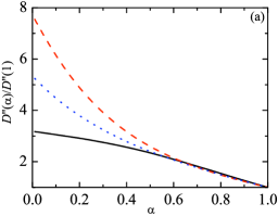
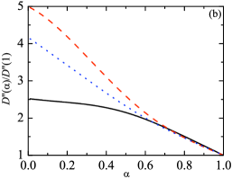
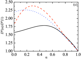
Figure 6: Plot of the reduced Duffour coefficient $D^{\prime\prime}(\alpha)/D(1)$ for hard spheres with $x_{1}=\frac{1}{2}$, $\sigma_{1}=\sigma_{2}$ and three different values of the mass ratio $\mu$: $\mu=2$ (a), $\mu=4$ (b), and $\mu=8$ (c). The solid lines correspond to the results obtained from the modified first Sonine approximation, the dashed lines refer to the results obtained from the standard first Sonine approximation while the dotted lines are the results derived by neglecting non-Gaussian corrections to the HCS distributions.

The shear viscosity $\eta$ is perhaps the most widely studied transport coefficient in granular fluids. Here, this coefficient has been measured in simulations by means of a new method proposed by the authors Montanero et al. (2005). This method is based on the simple shear flow state modified by the introduction of (i) a deterministic nonconservative force (Gaussian thermostat) that compensates for the collisional cooling and (ii) a stochastic process. While the Gaussian external force allows the granular mixture to reach a Newtonian regime where the (true) Navier-Stokes shear viscosity can be identified, the stochastic process is introduced to reproduce the conditions appearing in the CE solution to Navier-Stokes order. More details on this procedure can be found in Montanero et al. (2005). The simulation data obtained from this method along with both Sonine approximations are presented in Fig. 3 for disks ($d=2$) and spheres ($d=3$). We have considered again mixtures constituted by particles of the same mass density. The simulation data corresponding to $d=2$ for $\alpha\geq 0.5$ were reported by Garzó & Montanero (2007) while those corresponding to $d=3$ and $d=2$ for $\alpha\leq 0.5$ have been obtained in this work. As in the case of a single gas Garzó et al. (2007c), we observe that up to $\alpha\simeq 0.6$ the simulation data agree quite well with both theories. On the other hand, for higher inelasticities and in the physical three-dimensional case, the standard first Sonine approximation overestimates the shear viscosity while the modified first Sonine approximation compares well with computer simulations, even for low values of $\alpha$. We also observe that the improvement of the modified Sonine method over the standard one is less clear for hard disks ($d=2$) since the numerical data lie systematically between both theoretical approaches. However, even in this case the simulation results are closer to the modified ones than the standard ones. Therefore, according to the comparison carried out at the level of the coefficients $D$ and $\eta$, we can conclude that while the standard Sonine approximation does quite good a job for not strong values of dissipation, it is fair to say that the modified Sonine approximation is still better (especially for hard spheres) since is able to agree well with computer simulations in the full range of values of dissipation explored.

Let us consider finally the heat flux. As said in the Introduction, recent studies for a monocomponent gas Brey & Ruiz-Montero (2004); Brey et al. (2005a); Montanero et al. (2007) have shown that the standard first Sonine approximation dramatically overestimates the $\alpha$-dependence of the transport coefficients associated with the heat flux for high dissipation ($\alpha\lesssim 0.7$). This is the main reason why new alternative approximations Noskowicz et al. (2007) have been proposed. However, in contrast to the single gas case, the lack of available simulation data for granular mixtures for the coefficients $D^{\prime\prime}$, $L$ and $\lambda$ precludes a comparison between both Sonine approximations and computer simulations. Figures 4, 5 and 6 show the $\alpha$-dependence of the reduced transport coefficients $\lambda(\alpha)/\lambda(1)$, $L(\alpha)n/\lambda(1)$, and $D^{\prime\prime}(\alpha)/D^{\prime\prime}(1)$, respectively, for $d=3$, $x_{1}=\frac{1}{2}$, $\omega=1$ and different values of the mass ratio. Also for comparison we show the theoretical results obtained by neglecting non-Gaussian corrections to the HCS distributions $f_{i}^{(0)}$ [i.e., the cumulants given in (2) are neglected: $c_{i}=0$]. Simulation results reported by Brey & Ruiz-Montero (2004) for a monocomponent granular gas are also included in the case $\mu=1$, showing that the modified Sonine appoximation agrees with simulation data significantly better than the standard Sonine approximation, especially in the case of the pressure energy coefficient $L$. As expected, the standard and modified Sonine theories differ significantly for strong inelasticity, especially for mechanically different particles ($\mu\neq 1$). These discrepancies clearly justify the use of the modified Sonine approximation instead of the standard one to compute the dependence of the heat flux transport coefficients on dissipation. In addition, the standard approach leads to unphysical (negative) values for the thermal conductivity coefficient $\lambda$ for low values of $\alpha$, which is corrected by our modified Sonine approximation. This is of relevance, since it helps to clarify that the origin of unphysical values for the thermal conductivity at very high inelasticity is due to the mathematical accuracy of the Sonine approximation used and not to a more fundamental reason; an inherent lack of scale separation, for instance. Note also that the simple theoretical results Garzó & Montanero (2007) obtained by using Maxwellian forms for $f_{i}^{(0)}$ are even closer to the modified ones than those predicted by the standard approximation. The good agreement found in general between simulation (which yield the ”actual” values of the transport coefficients) and the modified Sonine approximation is a first evidence that the Chapman-Enskog method may be safely extended down to very low values of the coefficient of normal restitution $\alpha$.

5 Discussion

A modified Sonine approximation recently proposed Garzó et al. (2007c) for monocomponent systems has been extended to granular mixtures in this paper. This theory has been mainly motivated by the disagreement found at high dissipation Brey & Ruiz-Montero (2004); Brey et al. (2005a); Montanero et al. (2007) between the simulation data for the heat flux transport coefficients and the expressions derived from the standard first Sonine approximation for a single gas. As we have shown, important discrepancies between computer simulations and the standard Sonine approximation appear only in the region of strong inelasticity ($\alpha\lesssim 0.7$). Thus, it could be argued that the search for new theoretical methods may admittedly be more a mathematical than a physical endeavor. However, it is still physically relevant to propose methods Noskowicz et al. (2007); Garzó et al. (2007c) that produce accurate results for the transport coefficients in the complete range of possible values of the coefficients of restitution. As in the case of a monocomponent gas Garzó et al. (2007c), in the modified Sonine approximation the weight function for the unknowns ${\boldsymbol{\cal A}}_{i}$, ${\boldsymbol{\cal B}}_{i}$, ${\boldsymbol{\cal C}}_{i}$, and ${\boldsymbol{\cal D}}_{i}$ defining the first order distribution $f_{i}^{(1)}$ is not longer the Maxwell-Boltzmann distribution $f_{i,M}$ but the HCS distribution $f_{i}^{(0)}$. Moreover, in order to preserve the solubility conditions (21)–(23), the polynomial ${\boldsymbol{S}}_{i}({\boldsymbol{V}})$, defined by (24), appearing in the standard Sonine polynomial expansion must be replaced by the modified polynomial ${\overline{\boldsymbol{S}}}_{i}({\boldsymbol{V}})$, defined by (25). The idea behind the modified method is that the deviation of $f_{i}^{(0)}$ from $f_{i,M}$ has an important influence on the NS distribution $f_{i}^{(1)}$. In this context, it is expected that the rate of convergence of the Sonine polynomial expansion is accelerated when $f_{i}^{(0)}$ rather than $f_{i,M}$ is used as weight function.

The extension of the modified Sonine approach to mixtures is not easy at all since it involves the computation of new complex collision integrals. However, the structure of the NS transport coefficients is quite similar in the standard and modified approximations Garzó & Dufty (2002) since the distinction between both approximations occurs essentially in the $\alpha$-dependence of the characteristic collision frequencies of the transport coefficients $\nu_{D}$, $\tau_{ij}$, $\omega_{ij}$ and $\nu_{ij}$. The forms of the NS coefficients are given by equations (26)–(29) for the mass flux transport coefficients $D$, $D_{p}$, and $D^{\prime}$, equations (30)–(31b) for the shear viscosity $\eta$ and equations (32)–(37) for the heat flux transport coefficients $\lambda$, $L$, and $D^{\prime\prime}$. All the above expressions have the power to be explicit, namely, they are explicitly given in terms of the parameters of the mixture. A Mathematica code providing the NS transport coefficients under arbitrary values of composition, masses, sizes, and coefficients of restitution can be downloaded from our website . The fact that our theory does not involve numerical solutions allows us to evaluate the transport coefficients within very short computing times. For instance, the code using our theoretical expressions for the NS transport coefficients takes just of the order of 5 seconds in a standard personal computer to produce a graph similar to those in Fig. 6 of the most complicated heat flux transport coefficients . These results contrast with the method devised by Noskowicz et al. (2007) for a mocomponent gas where a system of algebraic equations must be numerically solved by employing the power of symbolic processors. This is perhaps another new added value of the method developed here for granular mixtures.

In order to check the accuracy of the modified Sonine approximation, computer simulations based on the DSMC method have been carried out in the cases of the tracer diffusion coefficient $D$ and the shear viscosity coefficient $\eta$. Although some simulation data for these coefficients were previously reported by the authors Garzó & Montanero (2004); Montanero et al. (2005), in this paper we extend those simulations to very low values of the coefficient of restitution (values of $\alpha$ typically larger than 0.1). This allows one to make a careful comparison between the modified and standard approximations with computer simulations. As expected, the discrepancies between simulation and the standard first Sonine estimates for $D$ and $\eta$ are partially corrected by the modified approximation, showing again the reliability of such approach for very strong values of dissipation. Unfortunatelly, the lack of available simulation data for the coefficients $\lambda$, $L$ and $D^{\prime\prime}$ corresponding to the heat flux precludes a comparison between theory and simulation for these transport coefficients, except in the single gas case Brey & Ruiz-Montero (2004); Brey et al. (2005a) where Figs. 5 and 6 show again the superiority of the modified Sonine approximation. We expect the present results for binary granular mixtures stimulates the performance of such simulations to assess the degree of accuracy of the modified Sonine method for the heat flux transport coefficients.

Hydrodynamic theories based on kinetic theory tools have been successful at predicting not only rapid granular flows (where the role of the interstitial fluid is assumed negligible), but have also been incorporated into models of high-velocity, gas-solid systems. These kinetic theory calculations are now standard features of commercial and research codes, such as Fluent${}^{\circledR}$ and MFIX (http://www.mfix.org/). These codes rely upon accurate expressions for the transport coefficients, and a first-order objective is to assure this accuracy from a careful treatment. As is shown in this paper, the price of this approach, in contrast to more phenomenological approaches, is an increasing complexity of the expressions for the transport coefficients as the system becomes more complex. In this context, we expect the theory reported here for granular binary mixtures to be quite useful for the above numerical codes.

The present results can be also applied to determine the dispersion relations for the hydrodynamic equations linearized about the homogeneous cooling state. Some previous results Garzó et al. (2006) based on the standard Sonine method have shown that the resulting equations exhibit a long wavelength instability for three of the modes. The objective now is to revisit the above problem by using the $\alpha$-dependence of the transport coefficients obtained in this paper (if this should be done, then for consistency reasons, the linearized Burnett corrections to the cooling rate would need to be considered in the hydrodynamic equations, since $\boldsymbol{\nabla}\boldsymbol{\cdot}\boldsymbol{j}_{1}^{(1)}$, $\boldsymbol{\nabla}_{l}\mathsfbi{P}_{kl}^{(1)}$ and $\boldsymbol{\nabla}\boldsymbol{\cdot}\boldsymbol{q}^{(1)}$ are of second order in the gradients, following the analysis by Brey et al. (1998)). Another possible open problem is to extend the present results (which are restricted to a low-density granular mixture) to finite densities in the framework of the Enskog kinetic theory. Given that the NS transport coefficients have been recently obtained from the Enskog equation Garzó et al. (2007a, b) by means of the standard Sonine approximation, it would be interesting to compare again the above results with those derived from the modified first Sonine method. Finally, it would also be interesting to devise a method to measure by means of Monte Carlo simulations some of the NS transport coefficients of the heat flux in a granular binary mixture. This method could be based on the method proposed by Montanero et al. (2007) for a single gas where the application of a homogeneous, anisotropic external force produces heat flux in the absence of gradients. We plan to carry out such extensions in the near future.

Appendix A Homogeneous cooling state

In this Appendix, the expressions of the cooling rate $\zeta^{(0)}$ and the fourth-degree cumulants $c_{i}$ are given. These expressions were reported by Garzó & Dufty (1999b) for inelastic hard spheres ($d=3$). Here, we extend these expressions to an arbitrary number of dimensions $d$.

By using the leading Sonine approximation (17) for $f_{1}^{(0)}$ and neglecting nonlinear terms in $c_{1}$ and $c_{2}$, the (reduced) cooling rate $\zeta_{1}^{*}\equiv\zeta_{1}^{(0)}/\nu_{0}$ (where $\nu_{0}=n\sigma_{12}^{d-1}v_{0}$) can be written as

$$\zeta_{1}^{*}=\zeta_{10}+\zeta_{11}c_{1}+\zeta_{12}c_{2},$$ (39)

where

$$\zeta_{10} = \frac{\sqrt{2}\pi^{(d-1)/2}}{d\Gamma\left(\frac{d}{2}\right)}x_{1}\left(\frac{\sigma_{1}}{\sigma_{12}}\right)^{d-1}\theta_{1}^{-1/2}(1-\alpha_{11}^{2})+\frac{4\pi^{(d-1)/2}}{d\Gamma\left(\frac{d}{2}\right)}x_{2}\mu_{21}$$ (40)

$$\times\left(\frac{1+\theta}{\theta}\right)^{1/2}(1+\alpha_{12})\theta_{2}^{-1/2}\left[1-\frac{1}{2}\mu_{21}(1+\alpha_{12})(1+\theta)\right],$$

$$\zeta_{11} = \frac{3\pi^{(d-1)/2}}{16\sqrt{2}d\Gamma\left(\frac{d}{2}\right)}x_{1}\left(\frac{\sigma_{1}}{\sigma_{12}}\right)^{d-1}\theta_{1}^{-1/2}(1-\alpha_{11}^{2})$$ (41)

$$+\frac{\pi^{(d-1)/2}}{8d\Gamma\left(\frac{d}{2}\right)}x_{2}\mu_{21}\frac{(1+\theta)^{-3/2}}{\theta^{1/2}}(1+\alpha_{12})\theta_{2}^{-1/2}\times$$

$$\left[2(3+4\theta)-3\mu_{21}(1+\alpha_{12})(1+\theta)\right],$$

$$\zeta_{12}=-\frac{\pi^{(d-1)/2}}{8d\Gamma\left(\frac{d}{2}\right)}x_{2}\mu_{21}\left(\frac{1+\theta}{\theta}\right)^{-3/2}(1+\alpha_{12})\theta_{2}^{-1/2}\left[2+3\mu_{21}(1+\alpha_{12})(1+\theta)\right].$$ (42)

In the above equations, $\mu_{ij}=m_{i}/(m_{i}+m_{j})$, $\theta_{1}=1/(\mu_{21}\gamma_{1})$, $\theta_{2}=1/(\mu_{12}\gamma_{2})$, $\theta=\theta_{1}/\theta_{2}$, and $v_{0}=\sqrt{2T(m_{1}+m_{2})/m_{1}m_{2}}$. The expression for $\zeta_{2}^{*}$ can be easily inferred from (40)–(42) by interchanging 1 and 2 and setting $\theta\to\theta^{-1}$.

The coefficients $c_{1}$ and $c_{2}$ are determined from the Boltzmann equations by multiplying them by $V^{4}$, and integrating over the velocity. After some algebra, when only linear terms in $c_{1}$ and $c_{2}$ are retained, the result is

$$c_{1}=\frac{AG-ED}{BG-DF},\quad c_{2}=\frac{BE-AF}{BG-DF},$$ (43)

where

$$A=-\frac{d(d+2)}{2\theta_{1}^{2}}\zeta_{10}-\Lambda_{1},\quad E=-\frac{d(d+2)}{2\theta_{2}^{2}}\zeta_{20}-\Lambda_{2},$$ (44)

$$D=\frac{d(d+2)}{2\theta_{1}^{2}}\zeta_{12}+\Lambda_{12},\quad F=\frac{d(d+2)}{2\theta_{2}^{2}}\zeta_{21}+\Lambda_{21},$$ (45)

$$B=\frac{d(d+2)}{2\theta_{1}^{2}}\left(\zeta_{11}+\frac{1}{2}\zeta_{10}\right)+\Lambda_{11},\quad G=\frac{d(d+2)}{2\theta_{2}^{2}}\left(\zeta_{22}+\frac{1}{2}\zeta_{20}\right)+\Lambda_{22}.$$ (46)

In the above equations, $\Lambda_{1}$, $\Lambda_{11}$ and $\Lambda_{12}$ are given by

$$\Lambda_{1} = -\frac{\pi^{(d-1)/2}}{\sqrt{2}\Gamma\left(\frac{d}{2}\right)}\theta_{1}^{-5/2}x_{1}\left(\frac{\sigma_{1}}{{\sigma}_{12}}\right)^{d-1}\frac{3+2d+2\alpha_{11}^{2}}{2}\left(1-\alpha_{11}^{2}\right)$$ (47)

$$+\frac{\pi^{(d-1)/2}}{\Gamma\left(\frac{d}{2}\right)}\theta_{1}^{-5/2}x_{2}\left(1+\theta\right)^{-1/2}\mu_{21}\left(1+\alpha_{12}\right)$$

$$\times\left\{-2\left[d+3+(d+2)\theta\right]+\mu_{21}\left(1+\alpha_{12}\right)\left(1+\theta\right)\left(11+d+\frac{d^{2}+5d+6}{d+3}\theta\right)\right.$$

$$\left.-8\mu_{21}^{2}\left(1+\alpha_{12}\right)^{2}\left(1+\theta\right)^{2}+2\mu_{21}^{3}\left(1+\alpha_{12}\right)^{3}\left(1+\theta\right)^{3}\right\}\;,$$

$$\Lambda_{11} = -\frac{\pi^{(d-1)/2}}{\sqrt{2}\Gamma\left(\frac{d}{2}\right)}\theta_{1}^{-5/2}x_{1}\left(\frac{\sigma_{1}}{{\sigma}_{12}}\right)^{d-1}\left[\frac{d-1}{2}(1+\alpha_{11})+\frac{3}{64}\left(10d+39+10\alpha_{11}^{2}\right)\left(1-\alpha_{11}^{2}\right)\right]$$ (48)

$$+\frac{\pi^{(d-1)/2}}{16\Gamma\left(\frac{d}{2}\right)}\theta_{1}^{-5/2}x_{2}\left(1+\theta\right)^{-5/2}\mu_{21}\left(1+\alpha_{12}\right)$$

$$\times\left\{-2\left[45+15d+(114+39d)\theta+(88+32d)\theta^{2}+(16+8d)\theta^{3}\right]\right.$$

$$+3\mu_{21}\left(1+\alpha_{12}\right)\left(1+\theta\right)\left[55+5d+9(10+d)\theta+4(8+d)\theta^{2}\right]$$

$$\left.-24\mu_{21}^{2}\left(1+\alpha_{12}\right)^{2}\left(1+\theta\right)^{2}\left(5+4\theta\right)+30\mu_{21}^{3}\left(1+\alpha_{12}\right)^{3}\left(1+\theta\right)^{3}\right\}\;,$$

$$\Lambda_{12} = \frac{\pi^{(d-1)/2}}{16\Gamma\left(\frac{d}{2}\right)}\theta_{1}^{-5/2}x_{2}\theta^{2}\left(1+\theta\right)^{-5/2}\mu_{21}\left(1+\alpha_{12}\right)$$ (49)

$$\times\left\{2\left[d-1+(d+2)\theta\right]+3\mu_{21}\left(1+\alpha_{12}\right)\left(1+\theta\right)\left[d-1+(d+2)\theta\right]\right.$$

$$\left.-24\mu_{21}^{2}\left(1+\alpha_{12}\right)^{2}\left(1+\theta\right)^{2}+30\mu_{21}^{3}\left(1+\alpha_{12}\right)^{3}\left(1+\theta\right)^{3}\right\}\;.$$

As before, the expressions for $\Lambda_{2}$, $\Lambda_{22}$ and $\Lambda_{21}$ are easily obtained from (47)–(49) by changing $1\leftrightarrow 2$. In the case of a three-dimensional system ($d=3$), all the above expressions reduce to those previously obtained for hard spheres Garzó & Dufty (1999b)

The dependence of the temperature ratio $\gamma=T_{1}/T_{2}$ on the parameters of the mixture is determined by requiring that the partial cooling rates $\zeta_{i}^{(0)}$ for the partial temperatures $T_{i}$ must be equal, i.e.,

$$\zeta_{1}^{(0)}=\zeta_{2}^{(0)}=\zeta^{(0)}.$$ (50)

Once equation (50) is solved, the cumulants $c_{i}$ are explicitly obtained by substituting $\gamma$ into (43).

Appendix B Expressions for the collision frequencies

The expressions of the different collision frequencies appearing in the NS transport coefficients are explicitly given in this Appendix. For their definitions please refer to the Supplementary Material file. The collision frequency $\nu_{D}$ associated to the the mass flux is given by

$$\nu_{D} = \frac{2\pi^{(d-1)/2}}{d\Gamma\left(\frac{d}{2}\right)}(1+\alpha_{12})\left(\frac{\theta_{1}+\theta_{2}}{\theta_{1}\theta_{2}}\right)^{1/2}\left\{x_{2}\mu_{21}\left[1+\frac{1}{16}\frac{\theta_{2}(3\theta_{2}+4\theta_{1})c_{1}-\theta_{1}^{2}c_{2}}{(\theta_{1}+\theta_{2})^{2}}\right]\right.$$ (51)

$$+\left.x_{1}\mu_{12}\left[1+\frac{1}{16}\frac{\theta_{1}(3\theta_{1}+4\theta_{2})c_{2}-\theta_{2}^{2}c_{1}}{(\theta_{1}+\theta_{2})^{2}}\right]\right\}.$$

It must be noted that the expression (51) for $\nu_{D}$ has been obtained by considering only linear terms in $c_{1}$ and $c_{2}$.

The expressions of the collision frequencies $\tau_{ij}$ corresponding to the shear viscosity are very long and so, for the sake of clarity, we have preferred to present them in terms of the operators $\Delta_{i}$ defined as

$$\Delta_{i}\equiv\theta_{i}^{2}\frac{\partial^{2}}{\partial\theta_{i}^{2}}+(d+2)\theta_{i}\frac{\partial}{\partial\theta_{i}}+\frac{d(d+2)}{4}.$$ (52)

Using (52), the collision frequencies $\tau_{11}$ and $\tau_{12}$ are given by

$$\tau_{11} = \frac{3\sqrt{2}\pi^{(d-1)/2}}{d(d+2)\Gamma\left(\frac{d}{2}\right)}x_{1}\left(\frac{\sigma_{1}}{{\sigma}_{12}}\right)^{d-1}(1+\alpha_{11})\theta_{1}^{-1/2}\left(1+\frac{2}{3}d-\alpha_{11}\right)\left(1+\frac{7}{32}c_{1}\right)$$ (53)

$$+\frac{2\pi^{(d-1)/2}}{d(d-1)(d+2)\Gamma\left(\frac{d}{2}\right)}x_{2}(1+\alpha_{12})\mu_{21}(\theta_{1}\theta_{2})^{d/2}\theta_{1}^{2}$$

$$\times\left[1-\frac{c_{1}}{4}(2-\Delta_{1})+\frac{c_{2}}{4}\Delta_{2}\right]I_{\eta}^{(11)}(\theta_{1},\theta_{2}),$$

$$\tau_{12}=\frac{2\pi^{(d-1)/2}}{d(d-1)(d+2)\Gamma\left(\frac{d}{2}\right)}x_{2} (1+\alpha_{12})\frac{\mu_{21}^{2}}{\mu_{12}}(\theta_{1}\theta_{2})^{d/2}\theta_{1}^{2}\times$$ (54)

$$\left[1-\frac{c_{2}}{4}(2-\Delta_{2})+\frac{c_{1}}{4}\Delta_{1}\right]I_{\eta}^{(12)}(\theta_{1},\theta_{2}),$$

where

$$I_{\eta}^{(11)}(\theta_{1},\theta_{2}) = (\theta_{1}\theta_{2})^{-\frac{d+1}{2}}\left\{2(d+3)(d-1)(\mu_{12}\theta_{2}-\mu_{21}\theta_{1})\theta_{1}^{-2}\left(\theta_{1}+\theta_{2}\right)^{-1/2}\right.$$ (55)

$$+3(d-1)\mu_{21}\left(1+\frac{2d}{3}-\alpha_{12}\right)\theta_{1}^{-2}\left(\theta_{1}+\theta_{2}\right)^{1/2}$$

$$\left.+\left[2d(d+1)-4\right]\theta_{1}^{-1}\left(\theta_{1}+\theta_{2}\right)^{-1/2}\right\},$$

$$I_{\eta}^{(12)}(\theta_{1},\theta_{2}) = (\theta_{1}\theta_{2})^{-\frac{d+1}{2}}\left\{2(d+3)(d-1)(\mu_{12}\theta_{2}-\mu_{21}\theta_{1})\theta_{2}^{-2}\left(\theta_{1}+\theta_{2}\right)^{-1/2}\right.$$ (56)

$$+3(d-1)\mu_{21}\left(1+\frac{2d}{3}-\alpha_{12}\right)\theta_{2}^{-2}\left(\theta_{1}+\theta_{2}\right)^{1/2}$$

$$\left.-\left[2d(d+1)-4\right]\theta_{2}^{-1}\left(\theta_{1}+\theta_{2}\right)^{-1/2}\right\}.$$

The corresponding expressions for $\tau_{22}$ and $\tau_{21}$ can be easily inferred from (54)–(56).

Let us consider now the NS transport coefficients $d_{i}^{*}$, $\ell_{i}^{*}$ and $\lambda_{i}^{*}$ of the heat flux. The quantities $Y_{i}$ appearing in the expressions (35)–(36) for these coefficients are given by

$$Y_{1}=\frac{D^{*}}{x_{1}\gamma_{1}^{2}}\left[\omega_{12}-\zeta^{*}\left(1+\frac{c_{1}}{2}\right)\right]-\frac{1}{\gamma_{1}^{2}}\left(\frac{\partial\gamma_{1}}{\partial x_{1}}\right)_{p,T}\left(1+\frac{c_{1}}{2}\right)-\frac{1}{2\gamma_{1}}\left(\frac{\partial c_{1}}{\partial x_{1}}\right)_{p,T},$$ (57)

$$Y_{2}=-\frac{D^{*}}{x_{2}\gamma_{2}^{2}}\left[\omega_{21}-\zeta^{*}\left(1+\frac{c_{2}}{2}\right)\right]-\frac{1}{\gamma_{2}^{2}}\left(\frac{\partial\gamma_{2}}{\partial x_{1}}\right)_{p,T}\left(1+\frac{c_{2}}{2}\right)-\frac{1}{2\gamma_{2}}\left(\frac{\partial c_{2}}{\partial x_{1}}\right)_{p,T},$$ (58)

$$Y_{3}=\frac{D_{p}^{*}}{x_{1}\gamma_{1}^{2}}\left[\omega_{12}-\zeta^{*}\left(1+\frac{c_{1}}{2}\right)\right]-\frac{m_{1}n}{\rho}\frac{c_{1}}{2\gamma_{1}^{2}},$$ (59)

$$Y_{4}=-\frac{D_{p}^{*}}{x_{2}\gamma_{2}^{2}}\left[\omega_{21}-\zeta^{*}\left(1+\frac{c_{2}}{2}\right)\right]-\frac{m_{2}n}{\rho}\frac{c_{2}}{2\gamma_{2}^{2}},$$ (60)

$$Y_{5}=\frac{D^{\prime*}}{x_{1}\gamma_{1}^{2}}\left[\omega_{12}-\zeta^{*}\left(1+\frac{c_{1}}{2}\right)\right]-\frac{1}{\gamma_{1}}\left(1+\frac{c_{1}}{2}\right),$$ (61)

$$Y_{6}=-\frac{D^{\prime*}}{x_{2}\gamma_{2}^{2}}\left[\omega_{21}-\zeta^{*}\left(1+\frac{c_{2}}{2}\right)\right]-\frac{1}{\gamma_{2}}\left(1+\frac{c_{2}}{2}\right),$$ (62)

where

$$\nu_{11} = \frac{8\pi^{(d-1)/2}}{d(d+2)\Gamma\left(\frac{d}{2}\right)}x_{1}\left(\frac{\sigma_{1}}{{\sigma}_{12}}\right)^{d-1}(1+\alpha_{11})(2\theta_{1})^{-1/2}\left[\frac{d-1}{2}+\frac{3}{16}(d+8)(1-\alpha_{11})\right.$$

$$\left.+\frac{296+217d-3(160+11d)\alpha_{11}}{512}c_{1}\right]$$

$$+\frac{\pi^{(d-1)/2}}{d(d+2)\Gamma\left(\frac{d}{2}\right)}x_{2}\mu_{21}(1+\alpha_{12})(\theta_{1}\theta_{2})^{d/2}\theta_{1}^{3}\left\{\left[1-\frac{c_{1}}{4}(d+8-\Delta_{1})+\frac{c_{2}}{4}\Delta_{2}\right]\right.$$

$$\times(\theta_{1}\theta_{2})^{-\frac{d+3}{2}}(\theta_{1}+\theta_{2})^{-3/2}E-(d+2)\theta_{1}^{-1}\left[1-\frac{c_{1}}{4}(d+8-\Delta_{1})+\frac{c_{2}}{4}\Delta_{2}\right]$$

$$\left.\times\theta_{1}^{-\frac{d+5}{2}}\theta_{2}^{-\frac{d+1}{2}}(\theta_{1}+\theta_{2})^{-1/2}[(d+2)\theta_{1}+(d+3)\theta_{2}]\right\}$$

$$-\frac{\pi^{(d-1)/2}}{d\Gamma\left(\frac{d}{2}\right)}x_{2}\mu_{21}(1+\alpha_{12})(\theta_{1}\theta_{2})^{d/2}\theta_{1}^{2}\left\{\left[1-\frac{c_{1}}{4}(d+8-\Delta_{1})+\frac{c_{2}}{4}\Delta_{2}\right]\right.$$

$$\times(\theta_{1}\theta_{2})^{-\frac{d+3}{2}}(\theta_{1}+\theta_{2})^{-1/2}A-(d+2)\theta_{1}^{-1}\left[1-\frac{c_{1}}{4}(d+8-\Delta_{1})+\frac{c_{2}}{4}\Delta_{2}\right]$$

$$\left.\times\theta_{1}^{-\frac{d+3}{2}}\theta_{2}^{-\frac{d+1}{2}}(\theta_{1}+\theta_{2})^{1/2}\right\}$$

$$-\frac{c_{1}}{2}\frac{\pi^{(d-1)/2}}{d\Gamma\left(\frac{d}{2}\right)}x_{2}\mu_{21}(1+\alpha_{12})(\theta_{1}+\theta_{2})^{-1/2}\theta_{1}^{1/2}\theta_{2}^{-3/2}\left[A-(d+2)\theta_{2}-(d+1)\theta_{1}^{-1}\theta_{2}^{2}\right],$$

$$\nu_{12} = -\frac{\pi^{(d-1)/2}}{d(d+2)\Gamma\left(\frac{d}{2}\right)}x_{2}\frac{\mu_{21}^{2}}{\mu_{12}}(1+\alpha_{12})(\theta_{1}\theta_{2})^{d/2}\theta_{1}^{3}\left\{\left[1-\frac{c_{2}}{4}(d+8-\Delta_{2})+\frac{c_{1}}{4}\Delta_{1}\right]\right.$$

$$\times(\theta_{1}\theta_{2})^{-\frac{d+3}{2}}(\theta_{1}+\theta_{2})^{-3/2}F-(d+2)\theta_{1}^{-1}\left[1-\frac{c_{2}}{4}(d+8-\Delta_{2})+\frac{c_{1}}{4}\Delta_{1}\right]$$

$$\left.\times\theta_{1}^{-\frac{d+1}{2}}\theta_{2}^{-\frac{d+5}{2}}(\theta_{1}+\theta_{2})^{-1/2}[(d+3)\theta_{1}+(d+2)\theta_{2}]\right\}$$

$$-\frac{\pi^{(d-1)/2}}{d\Gamma\left(\frac{d}{2}\right)}x_{2}\frac{\mu_{21}^{2}}{\mu_{12}}(1+\alpha_{12})\theta_{1}^{3+\frac{d}{2}}\theta_{2}^{\frac{d}{2}-1}\left\{\left[1-\frac{c_{2}}{4}(d+8-\Delta_{2})+\frac{c_{1}}{4}\Delta_{1}\right]\right.$$

$$\times(\theta_{1}\theta_{2})^{-\frac{d+3}{2}}(\theta_{1}+\theta_{2})^{-1/2}B+(d+2)\theta_{1}^{-1}$$

$$\left.\left[1-\frac{c_{2}}{4}(d+8-\Delta_{2})+\frac{c_{1}}{4}\Delta_{1}\right]\theta_{1}^{-\frac{d+1}{2}}\theta_{2}^{-\frac{d+3}{2}}(\theta_{1}+\theta_{2})^{1/2}\right\}$$

$$-\frac{\pi^{(d-1)/2}}{2d\Gamma\left(\frac{d}{2}\right)}x_{2}\frac{\mu_{21}^{2}}{\mu_{12}}(1+\alpha_{12})(\theta_{1}+\theta_{2})^{-1/2}\theta_{1}^{3/2}\theta_{2}^{-5/2}\left[c_{2}B+c_{2}(d+2)(\theta_{1}+\theta_{2})-c_{1}\theta_{2}\right],$$

$$\omega_{12} = \frac{\sqrt{2}\pi^{(d-1)/2}}{d\Gamma\left(\frac{d}{2}\right)}x_{1}\left(\frac{\sigma_{1}}{{\sigma}_{12}}\right)^{d-1}\theta_{1}^{-1/2}(1+\alpha_{11})\left[1-\alpha_{11}+\frac{70+47d-3(34+5d)\alpha_{11}}{32(d+2)}c_{1}\right]$$ (65)

$$+\frac{2\pi^{(d-1)/2}}{d(d+2)\Gamma\left(\frac{d}{2}\right)}\mu_{21}(1+\alpha_{12})\theta_{1}^{2}(\theta_{1}\theta_{2})^{d/2}\times$$

$$\left[x_{2}\left(1+\frac{c_{1}}{4}\Delta_{1}+\frac{c_{2}}{4}\Delta_{2}\right)(\theta_{1}\theta_{2})^{-\frac{d+3}{2}}(\theta_{1}+\theta_{2})^{-1/2}A\right.$$

$$\left.-x_{1}\frac{\mu_{12}}{\mu_{21}}\theta_{2}\theta_{1}^{-1}\left(1+\frac{c_{1}}{4}\Delta_{1}+\frac{c_{2}}{4}\Delta_{2}\right)(\theta_{1}\theta_{2})^{-\frac{d+3}{2}}(\theta_{1}+\theta_{2})^{-1/2}B\right.$$

$$-(d+2)\theta_{1}^{-1}x_{2}\left(1+\frac{c_{1}}{4}\Delta_{1}+\frac{c_{2}}{4}\Delta_{2}\right)\theta_{1}^{-\frac{d+3}{2}}\theta_{2}^{-\frac{d+1}{2}}(\theta_{1}+\theta_{2})^{1/2}$$

$$\left.-(d+2)x_{1}\frac{\mu_{12}}{\mu_{21}}\theta_{2}\theta_{1}^{-2}\left(1+\frac{c_{1}}{4}\Delta_{1}+\frac{c_{2}}{4}\Delta_{2}\right)\theta_{1}^{-\frac{d+1}{2}}\theta_{2}^{-\frac{d+3}{2}}(\theta_{1}+\theta_{2})^{1/2}\right]$$

$$-c_{1}\frac{\pi^{(d-1)/2}}{d\Gamma\left(\frac{d}{2}\right)}(1+\alpha_{12})\left(\frac{\theta_{1}+\theta_{2}}{\theta_{1}\theta_{2}}\right)^{1/2}\left(x_{2}\mu_{21}+x_{1}\mu_{12}\right).$$

In the above equations we have introduced the quantities

$$A(\theta_{1},\theta_{2}) = (d+2)(2\beta_{12}+\theta_{2})+\mu_{21}(\theta_{1}+\theta_{2})\times$$

$$\left\{(d+2)(1-\alpha_{12})-[(11+d)\alpha_{12}-5d-7]\beta_{12}\theta_{1}^{-1}\right\}$$

$$+3(d+3)\beta_{12}^{2}\theta_{1}^{-1}+2\mu_{21}^{2}\left(2\alpha_{12}^{2}-\frac{d+3}{2}\alpha_{12}+d+1\right)\theta_{1}^{-1}(\theta_{1}+\theta_{2})^{2},$$

$$B(\theta_{1},\theta_{2}) = (d+2)(2\beta_{12}-\theta_{1})+\mu_{21}(\theta_{1}+\theta_{2})\times$$

$$\left\{(d+2)(1-\alpha_{12})+[(11+d)\alpha_{12}-5d-7]\beta_{12}\theta_{2}^{-1}\right\}$$

$$-3(d+3)\beta_{12}^{2}\theta_{2}^{-1}-2\mu_{21}^{2}\left(2\alpha_{12}^{2}-\frac{d+3}{2}\alpha_{12}+d+1\right)\theta_{2}^{-1}(\theta_{1}+\theta_{2})^{2},$$

$$E(\theta_{1},\theta_{2}) = 2\mu_{21}^{2}\theta_{1}^{-2}(\theta_{1}+\theta_{2})^{2}\left(2\alpha_{12}^{2}-\frac{d+3}{2}\alpha_{12}+d+1\right)\left[(d+2)\theta_{1}+(d+5)\theta_{2}\right]$$ (68)

$$-\mu_{21}(\theta_{1}+\theta_{2})\left\{\beta_{12}\theta_{1}^{-2}[(d+2)\theta_{1}+(d+5)\theta_{2}][(11+d)\alpha_{12}-5d-7]\right.$$

$$\left.-\theta_{2}\theta_{1}^{-1}[20+d(15-7\alpha_{12})+d^{2}(1-\alpha_{12})-28\alpha_{12}]-(d+2)^{2}(1-\alpha_{12})\right\}$$

$$+3(d+3)\beta_{12}^{2}\theta_{1}^{-2}[(d+2)\theta_{1}+(d+5)\theta_{2}]$$

$$+2\beta_{12}\theta_{1}^{-1}[(d+2)^{2}\theta_{1}+(24+11d+d^{2})\theta_{2}]$$

$$+(d+2)\theta_{2}\theta_{1}^{-1}[(d+8)\theta_{1}+(d+3)\theta_{2}],$$

$$F(\theta_{1},\theta_{2}) = 2\mu_{21}^{2}\theta_{2}^{-2}(\theta_{1}+\theta_{2})^{2}\left(2\alpha_{12}^{2}-\frac{d+3}{2}\alpha_{12}+d+1\right)\left[(d+5)\theta_{1}+(d+2)\theta_{2}\right]$$ (69)

$$-\mu_{21}(\theta_{1}+\theta_{2})\left\{\beta_{12}\theta_{2}^{-2}[(d+5)\theta_{1}+(d+2)\theta_{2}][(11+d)\alpha_{12}-5d-7]\right.$$

$$\left.+\theta_{1}\theta_{2}^{-1}[20+d(15-7\alpha_{12})+d^{2}(1-\alpha_{12})-28\alpha_{12}]+(d+2)^{2}(1-\alpha_{12})\right\}$$

$$+3(d+3)\beta_{12}^{2}\theta_{2}^{-2}[(d+3)\theta_{1}+(d+2)\theta_{2}]$$

$$-2\beta_{12}\theta_{2}^{-1}[(24+11d+d^{2})\theta_{1}+(d+2)^{2}\theta_{2}]$$

$$+(d+2)\theta_{1}\theta_{2}^{-1}[(d+3)\theta_{1}+(d+8)\theta_{2}].$$

Here, $\beta_{12}=\mu_{12}\theta_{2}-\mu_{21}\theta_{1}$. From (B)–(69), one easily gets the expressions for $\omega_{21}$, $\nu_{22}$ and $\nu_{21}$ by interchanging $1\leftrightarrow 2$.

Finally, note that the expressions (51), (53), (54), (B), (B), and (65) reduce to those previously obtained Garzó & Montanero (2007) when one takes Maxwellians distributions for the reference homogeneous cooling state $f_{i}^{(0)}$, i.e., when $c_{1}=c_{2}=0$. Moreover, in the case of mechanically equivalent particles, the expressions of $\nu_{D}$, $\tau_{ij}$ and $\nu_{ij}$ are consistent with those recently obtained for a monocomponent gas by using the modified Sonine approximation Garzó et al. (2007c).

References

- Aranson & Tsimring (2006) Aranson, I. S. & Tsimring, L. V. 2006 Patterns and collective behaviour in granular media: Theoretical concepts. Rev. Mod. Phys. 78, 641–692.
- Arnarson & Willits (1998) Arnarson, B. & Willits, J. T. 1998 Thermal diffusion in binary mixtures of smooth, nearly elastic spheres with and without gravity. Phys. Fluids. 10, 1324–1328.
- Barrat & Trizac (2002) Barrat, A. & Trizac, E. 2002 Lack of energy equipartition in homogeneous heated binary granular mixtures. Gran. Matt. 4, 57–63.
- Bird (1994) Bird, G. A. 1994 Molecular Gas Dynamics and the Direct Simulation Monte Carlo of Gas Flows. Clarendon, Oxford.
- Brey et al. (1997) Brey, J. J., Dufty, J. W. & Santos, A. 1997 Dissipative dynamics for hard spheres. J. Stat. Phys. 87, 1051–1066.
- Brey et al. (1998) Brey, J. J., Dufty, J. W., Santos, A. & Kim, C. S. 1998 Hydrodynamics for granular flows at low density. Phys. Rev. E 58, 4638–4653.
- Brey & Ruiz-Montero (2004) Brey, J. J. & Ruiz-Montero, M. J. 2004 Simulation study of the Green-Kubo relations for dilute granular gases. Phys. Rev. E 70, 051301.
- Brey et al. (1999) Brey, J. J., Ruiz-Montero, M. J. & Cubero, D. 1999 On the validity of linear hydrodynamics for low-density granular flows described by the Boltzmann equation. Europhys. Lett. 48, 359–364.
- Brey et al. (2000) Brey, J. J., Ruiz-Montero, M. J., Cubero, D. & García-Rojo, R. 2000 Self-diffusion in freely evolving granular gases. Phys. Fluids. 12, 876–883.
- Brey et al. (2005a) Brey, J. J., Ruiz-Montero, M. J., Maynar, P. & García de Soria, I. 2005a Hydrodynamic modes, Green-Kubo relations, and velocity correlations in dilute granular gases. J. Phys.: Condens. Matter 17 (S2502).
- Brey et al. (2005b) Brey, J. J., Ruiz-Montero, M. J. & Moreno, F. 2005b Energy partition and segregation for an intruder in a vibrated granular system under gravity. Phys. Rev. Lett. 95, 098001.
- Brey et al. (2006) Brey, J. J., Ruiz-Montero, M. J. & Moreno, F. 2006 Hydrodynamic profiles for an impurity in an open vibrated granular gas. Phys. Rev. E 73, 031301.
- Brey et al. (2002) Brey, J. J., Ruiz-Montero, M. J., Moreno, F. & García-Rojo, R. 2002 Transversal inhomogeneities in dilute vibrofluidized granular fluids. Phys. Rev. E 65, 061302.
- Brilliantov & Pöschel (2004) Brilliantov, N. & Pöschel, T. 2004 Kinetic Theory of Granular Gases. Oxford University Press.
- Chapman & Cowling (1970) Chapman, S. & Cowling, T. G. 1970 The Mathematical Theory of Nonuniform Gases. Cambridge University Press.
- Clerc et al. (2008) Clerc, M. G., Cordero, P., Dunstan, J., Huff, K., Mujica, N., Risso, D. & Varas, G. 2008 Liquid-solid-like transition in quasi-one-dimensional driven granular media. Nature Phys. 4, 249–254.
- Dahl et al. (2002) Dahl, S. R., Hrenya, C. M., Garzó, V. & Dufty, J. W. 2002 Kinetic temperatures for a granular mixture. Phys. Rev. E 66, 041301.
- Feitosa & Menon (2002) Feitosa, K. & Menon, N. 2002 Breakdown of energy equipartition in a 2d binary vibrated granular gas. Phys. Rev. Lett. 88, 198301.
- Garzó (2005) Garzó, V. 2005 Instabilities in a free granular fluid described by the Enskog equation. Phys. Rev. E 72, 021106.
- Garzó & Dufty (1999a) Garzó, V. & Dufty, J. W. 1999a Dense fluid transport for inelastic hard spheres. Phys. Rev. E 59, 5895–5911.
- Garzó & Dufty (1999b) Garzó, V. & Dufty, J. W. 1999b Homogeneous cooling state for a granular mixture. Phys. Rev. E 60, 5706–5713.
- Garzó & Dufty (2002) Garzó, V. & Dufty, J. W. 2002 Hydrodynamics for a granular binary mixture at low density. Phys. Fluids. 14, 1476–1490.
- Garzó et al. (2007a) Garzó, V., Dufty, J. W. & Hrenya, C. M. 2007a Enskog theory for polydisperse granular mixtures. I. Navier-Stokes order transport. Phys. Rev. E 76, 031303.
- Garzó et al. (2007b) Garzó, V., Hrenya, C. M. & Dufty, J. W. 2007b Enskog theory for polydisperse granular mixtures II. Sonine polynomial approximation. Phys. Rev. E 76, 031304.
- Garzó & Montanero (2002) Garzó, V. & Montanero, J. M. 2002 Transport coefficients of a heated granular gas. Physica A 313, 336–356.
- Garzó & Montanero (2004) Garzó, V. & Montanero, J. M. 2004 Diffusion of impurities in a granular gas. Phys. Rev. E 69, 021301.
- Garzó & Montanero (2007) Garzó, V. & Montanero, J. M. 2007 Navier-Stokes transport coefficients of -dimensional granular binary mixtures at low-density. J. Stat. Phys. 129, 27–58.
- Garzó et al. (2006) Garzó, V., Montanero, J. M. & Dufty, J. W. 2006 Mass and heat fluxes for a binary granular mixture at low-density. Phys. Fluids. 18, 083305.
- Garzó & Santos (2003) Garzó, V. & Santos, A. 2003 Kinetic Theory of Gases in Shear Flows. Nonlinear Transport. Kluwer Academic Publishers.
- Garzó et al. (2007c) Garzó, V., Santos, A. & Montanero, J. M. 2007c Modified Sonine approximation for the Navier-Stokes transport coefficients of a granular gas. Physica A 376, 94–107.
- Goldhirsch (2003) Goldhirsch, I. 2003 Rapid granular flows. Annu. Rev. Fluid Mech. 22, 57–92.
- Goldshtein & Shapiro (1995) Goldshtein, A. & Shapiro, M. 1995 Mechanics of collisional motion of granular materials. Part 1. General hydrodynamic equations. J. Fluid Mech. 282, 75–114.
- Hrenya et al. (2008) Hrenya, C. M., Galvin, J. E. & Wildman, R. D. 2008 Evidence of higher-order effects in thermally driven granular flows. J. Fluid Mech. 598, 429–450.
- Huan et al. (2004) Huan, C., Yang, X., Candela, D., Mair, R. W. & Walsworth, R. L. 2004 NMR experiments on a three-dimensional vibrofluidized granular medium. Phys. Rev. E 69, 041302.
- Jenkins & Mancini (1989) Jenkins, J. T. & Mancini, F. 1989 Kinetic theory for binary mixtures of smooth, nearly elastic spheres. Phys. Fluids. A 1, 2050–2057.
- Krouskop & Talbot (2003) Krouskop, P. & Talbot, J. 2003 Mass and size effects in three-dimensional vibrofluidized granular mixtures. Phys. Rev. E 68, 021304.
- Lois et al. (2007) Lois, G., Lemaître, A. & Carlson, J. M. 2007 Spatial force correlations in granular shear flow. ii. Theoretical implications. Phys. Rev. E 76, 021303.
- Lutsko (2005) Lutsko, J. 2005 Transport properties of dense dissipative hard-sphere fluids for arbitrary energy loss models. Phys. Rev. E 72, 021306.
- Lutsko et al. (2002) Lutsko, J., Brey, J. J. & Dufty, J. W. 2002 Diffusion in a granular fluid. II. Simulation. Phys. Rev. E 65, 051304.
- Montanero & Garzó (2002) Montanero, J. M. & Garzó, V. 2002 Monte Carlo simulation of the homogeneous cooling state for a granular mixture. Gran. Matt. 4, 17–24.
- Montanero & Garzó (2003) Montanero, J. M. & Garzó, V. 2003 Shear viscosity for a heated granular binary mixture at low-density. Phys. Rev. E 67, 021308.
- Montanero et al. (2005) Montanero, J. M., Santos, A. & Garzó, V. 2005 DSMC evaluation of the Navier-Stokes shear viscosity of a granular fluid. In Rarefied Gas Dynamics 24 (ed. AIP Conference Proceedings), , vol. 762, pp. 797–802.
- Montanero et al. (2007) Montanero, J. M., Santos, A. & Garzó, V. 2007 First-order Chapman-Enskog velocity distribution function in a granular gas. Physica A 376, 75–93.
- Noskowicz et al. (2007) Noskowicz, S. H., Bar-Lev, O., Serero, D. & Goldhirsch, I. 2007 Computer-aided kinetic theory and granular gases. Europhys. Lett. 79, 60001.
- Pagnani et al. (2002) Pagnani, R., Marconi, U. M. B. & Puglisi, A. 2002 Driven low density granular mixtures. Phys. Rev. E 66, 051304.
- Rericha et al. (2002) Rericha, E. C., Bizon, C., Shattuck, M. D. & Swinney, H. L. 2002 Shocks in supersonic sand. Phys. Rev. Lett. 88, 014302.
- Santos et al. (2004) Santos, A., Garzó, V. & Dufty, J. W. 2004 Inherent rheology of a granular fluid in uniform shear flow. Phys. Rev. E 69, 061303.
- Schröter et al. (2006) Schröter, M., Ulrich, S., Kreft, J., Swift, J. B. & Swinney, H. L. 2006 Mechanisms in the size segregation of a binary granular mixture. Phys. Rev. E 74, 011307.
- Sela & Goldhirsch (1998) Sela, N. & Goldhirsch, I. 1998 Hydrodynamic equations for rapid flows of smooth inelastic spheres to Burnett order. J. Fluid Mech. 361, 41–74.
- Serero et al. (2006) Serero, D., Goldhirsch, I., Noskowicz, S. H. & Tan, M. L. 2006 Hydrodynamics of granular gases and granular gas mixtures. J. Fluid Mech. 554, 237–258.
- Vega Reyes & Urbach (2008a) Vega Reyes, F. & Urbach, J. S. 2008a The effect of inelasticity on the phase transitions of a thin vibrated granular layer. Phys. Rev. E 78, 051301.
- Vega Reyes & Urbach (2008b) Vega Reyes, F. & Urbach, J. S. 2008b Steady base states for Navier-Stokes granulodynamics with boundary heating and shear. J. Fluid. Mech. (submitted). Preprint: arXiv: 0807.5125.
- Wang et al. (2003) Wang, H., Jin, G. & Ma, Y. 2003 Simulation study on kinetic temperatures of vibrated binary granular mixtures. Phys. Rev. E 68, 031301.
- Wildman & Parker (2002) Wildman, R. D. & Parker, D. J. 2002 Coexistence of two granular temperatures in binary vibrofluidized beds. Phys. Rev. Lett. 88, 064301.
- Willits & Arnarson (1999) Willits, J. T. & Arnarson, B. 1999 Kinetic theory of a binary mixture of nearly elastic disks. Phys. Fluids. 11, 3116–3122.
- Yang et al. (2002) Yang, X., Huan, C., Candela, D., Mair, R. W. & Walsworth, R. L. 2002 Measurements of grain motion in a dense, three-dimensional granular fluid. Phys. Rev. Lett. 88, 044301.
- Zamankhan (1995) Zamankhan, Z. 1995 Kinetic theory for multicomponent dense mixtures of slightly inelastic spherical particles. Phys. Rev. E 52, 4877–4891.