Spin-Polarized STM for a Kondo adatom
Abstract
We investigate the bias dependence of the tunneling conductance between a spin-polarized (SP) scanning tunneling microscope (STM) tip and the surface conduction states of a normal metal with a Kondo adatom. Quantum interference between tip-host metal and tip-adatom-host metal conduction paths is studied in the full range of the Fano parameter . The spin-polarized STM gives rise to a splitting of the Kondo peak and asymmetry in the zero-bias anomaly depending on the lateral tip-adatom distance. For increasing lateral distances, the Kondo peak-splitting shows a strong suppression and the spin-polarized conductance exhibits the standard Fano-Kondo profile.
1 Introduction
The Kondo effect is an antiferromagnetic screening of a localized magnetic moment by the host metallic electrons below a characteristic Kondo temperature , which results in the appearance of an additional peak in the system’s density of states pinned to the Fermi energy. Being first observed during studies of transport properties of bulk diluted magnetic alloys [1], the Kondo effect was later on shown to affect the conductance of single quantum dots (QDs) [2, 3], arrays of QDs [4, 5] and possibly quantum point contacts [6, 7]. In the emerging field of spintronics [8], the coupling of a single QD to ferromagnetic leads can shed more light on fundamental aspects of the Kondo physics and provide a basis for a design of novel spintronic composants [9, 10, 11, 12, 13, 14, 15, 16, 17].
The Scanning Tunneling Microscope (STM) is widely used for investigation of the Kondo effect at surfaces of normal metals with adsorbed magnetic impurities (Kondo adatoms) [18, 19, 20, 21, 22, 23, 24, 25, 26]. The possible examples are individual Co atoms at Au(111), Cu(100) or Cu(111) surfaces [18, 19, 20, 21], and cobalt carbonyl Co(CO)n complexes or manganese phthalocyanine (MnPc) molecules on top of Pb islands [22, 23].
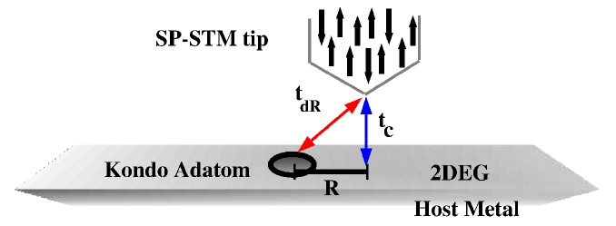
In the present work we focus on the Kondo regime for a system containing a ferromagnetic STM tip and a single Kondo adatom on a metallic surface (figure 1). In this system the conductance becomes spin dependent, due to the ferromagnetic (FM) tip, which leads to a Zeeman splitting in the Kondo adatom density of states (DOS). Particular attention is payed to the interplay between Kondo effect, quantum interference of two possible tunneling paths (tip-adatom-host and tip-host) and the ferromagnetism of the tip.
Our study differs from previous work in the same field [27] mainly in the three aspects described below.
First. We present new results for the tunneling conductance as a function of the bias for different lateral tip-adatom separations R in the Kondo regime. This is an actual task indeed, as in experiments with unpolarized systems, R was shown to strongly affect the conductance [18, 19]. For ferromagnetic tips, however, correspondent results are lacking.
Second. We discuss the small, large and intermediate cases for the Fano parameter [28, 29, 30, 31, 32]. We show that the three cases above give different conductance patterns. Experimentally, the large and small limits are relevant and have been realized for unpolarized conduction bands. For example, in reference [21] it was shown that alternates from intermediate () to small () values by changing the Cu crystal surface (Cu(100) and Cu(111)), in which a Co adatom is deposited. The conductance profile for small limit can also be experimentally observed in quantum corrals [19]. Alternatively, manipulating the molecular structure of the magnetic impurity on the Cu(100) surface, it is possible to switch between the intermediate and large limits [22, 23].
Third. Instead of using a Lorentzian approximation for the Kondo peak, we apply the well established Doniach-Sunjic formula [33, 34], whose validity is supported by numerical calculations based on both numerical renormalization group [33, 34], quantum Monte Carlo simulations [35] and by the recent success in fitting experimental data [23].
Our results show that for a tip situated right above the Kondo adatom (R=0) an asymmetric zero-bias anomalies appear, which are revealed as resonances and anti-resonances in the conductance in the limits of large and small , respectively. For , the conductance demonstrates a pronounced plateau in the region of small biases (). The increase of leads to a suppression of the tip-induced adatom’s Zeeman splitting, thus resulting in a conductance pattern that resembles experimental data for unpolarized systems [18]. Finally, we verify that the Kondo peak splitting strongly depends on the asymmetry between the tip-adatom and adatom-host tunnelings.
The paper is organized as follow. In section 1 we present the model adopted to describe the system under study. In section 2 we derive an expression for the spin-resolved conductance based on a perturbative expansion for the tunneling Hamiltonian. In section 3 we discuss the numerical results. Conclusions are present in section 4.
2 The Model
The description of the metallic host and its interaction with the adatom is performed within the framework of the single impurity Anderson model [36] with a half-filled noninteracting conduction band,
| (1) | |||||
where all energies are measured from the Fermi level coinciding with the center of the band and extend from to . The operator
| (2) |
corresponds to a surface conduction state of the host metal with an energy-independent density of states per spin .
The first term in equation (1) describes a two dimensional electron gas (2DEG) on the surface of a host metal. The second and the third correspond to the adatom, which is characterized by a single particle orbital energy and Coulomb repulsion . The last term, proportional to describes the coupling between the adatom and the host metal conduction states, thus introducing the broadenings of the adatom’s resonances at the energies and In the Kondo regime (, , ) an additional peak in the density of states having a half-width , ( is the Boltzmann constant and the Kondo temperature) [37] appears exactly at the Fermi level.
The total STM Hamiltonian reads
| (3) |
where corresponds to free electrons in the tip,
| (4) |
with the operators describing the bulk conduction states, the bias is and
| (5) |
is the tunneling Hamiltonian that connects the tip with the host metal via the operator
| (6) |
The normalization factor in equation (6) reads
| (7) |
with being a wave function of the host conduction electron.
The first term in equation (6) containing the operator
| (8) |
hybridizes the conduction states of the tip with the surface of the host at a displaced lateral position from the adatom.
The second term describes the tunneling between the tip and localized adatom’s level characterized by a spin-dependent parameter (Fano factor) [38, 39]
| (9) |
defined as a ratio between the couplings of the tip-adatom and of the tip-host metal.
The Fano factor monitors the competition between the tunneling channels in the system. It vanishes with the increase of the tip-adatom lateral distance , which can be modeled by an exponentially decaying function [39]
| (10) |
The decay of the Fano parameter with the increasing of the lateral tip-adatom distance was already experimentally explored in a system with a Co adatom on a Cu surface [21].
In the present work we consider a ferromagnetic tip with a spin-dependent density of states given by
| (11) |
where or for spins or , respectively, is a polarization degree of the tip. The inequality between spin-up and spin-down populations in the tip introduces an asymmetry in the splitting of the zero-bias anomaly as we will see in Sec. IV. The density of states for the unpolarized tip is assumed to be equal to the density of states of the host metal for simplicity.
3 Methodology
We calculate the tunneling conductance of the system treating the coupling between tip and host metal as a perturbation. Within a second order perturbation scheme, the formula for the conductance [38] reads
| (12) |
where
| (13) |
is an effective transmission coefficient with
| (14) |
The local density of states (LDOS) appearing in equation (13) is defined as
| (15) |
with being the retarded Green function thermally averaged over the eigenstates of the Hamiltonian (1).
Looking at equation (15), one sees that the LDOS depends on non-orthonormal fermionic operators
| (16) |
where the spatial function is given by
| (17) |
with being the 0-th order Bessel function.
The operator (6) can be expressed in terms of fermionic operators orthonormal to by introducing
| (18) |
with a normalization factor evaluated at the Fermi level,
| (19) |
This leads to the following expression for ,
where we introduce an operator
| (21) |
which describes a conduction state centered at the adatom site.
As the Kondo effect occurs at low temperatures and the tip bias is usually much smaller then the bandwidth, , we evaluate equation (12) at , thus resulting in
| (22) |
where
| (23) |
and
| (24) | |||||
In the calculation of the above expression we used the Green function identities for zero temperature Anderson model [36]. The spin dependent Fano factor phase shift is defined as
| (25) |
In equation (24) the terms proportional to and come from the direct tunneling paths tip-adatom-host and tip-host, respectively. The interference between then is given by the mixture term proportional to
The spin dependent phase shift for the conduction states can be determined from the Doniach-Sunjic spectral density [33, 34]
| (26) |
where gives the Kondo peak splitting, which is related to the adatom energy level as
| (27) |
where is the adatom level without magnetic field. According to “poor man’s” scaling [11], such splitting can be estimated as [40]
| (28) | |||||
where gives the local coupling between the Kondo adatom and an unpolarized tip. We use the expression
| (29) |
to account for both spin and spatial dependencies of the tip-adatom coupling.
4 Results
For numerical analysis we adopt the following set of model parameters: eV, eV, eV, eV, K and Å-1 [26, 27]. We consider the cases of large, small and intermediate Fano ratio values. For each of these cases we analyze the dependence of the conductance on tip-adatom lateral distance . Additionally, for large limit we consider how the conductance depends on the asymmetry between tip-adatom and adatom-host couplings.
4.1 Large tip-adatom coupling ()
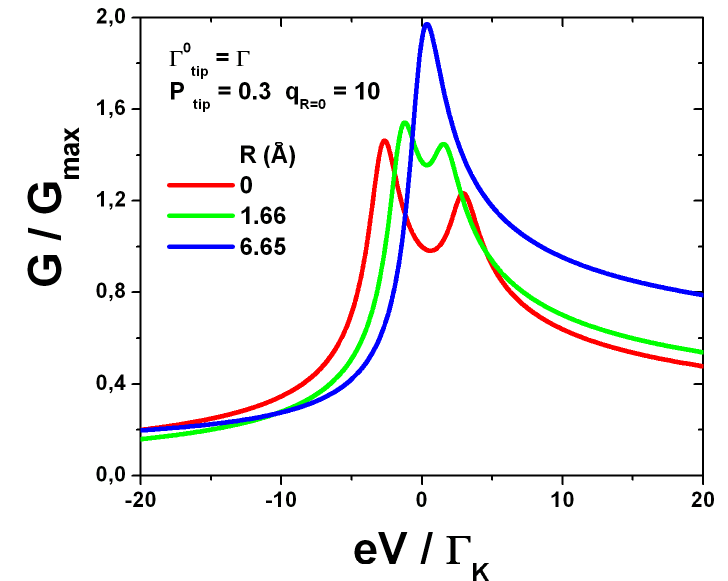
The large limit has been achieved in experiments with STM tip by employing magnetic molecules as Kondo adatoms [22, 23]. In this limit the host metal conduction electrons tunnel towards the tip preferably via the localized magnetic adatom state. For the tip situated right above the adatom , the conductance reveals an asymmetric splitting of the zero bias anomaly (figure (2)), characterized by a pair of peaks at and . Such asymmetry occurs due to the spin polarization of the tip (equation (11)), the higher peak corresponding to the majority spin up states, while the lower one to the minority spin down states.
A similar asymmetric splitting of the Kondo peak was recently observed in a quantum dot system coupled to two ferromagnetic Ni electrodes [16, 17]. The large limit in the system we consider resembles the standard case of a single dot in between leads without lead-to-lead direct coupling (embedded geometry). A wealth of theoretical works predict the spin splitting of the Kondo peak in a quantum dot system coupled to two ferromagnetic leads [10, 11, 15]. In those works this splitting was tuned via the relative angle between the left and the right lead magnetization [15], the leads polarization [10] and an external magnetic field [11]. Here we show one alternative/additional way to tune the spin splitting, by changing the tip-adatom separation (laterally or vertically) [41].
Increasing the tip-adatom lateral distance, the Fano ratio decays according to equation (10) and the Zeeman splitting of the Kondo peak quenches (see equation (28)). These effects can be seen at figure (2), where the conductance is plotted for three different values of the tip-adatom lateral distance. About Å, the two resonances merge into a single peak, thus resulting in the standard Kondo resonance profile.
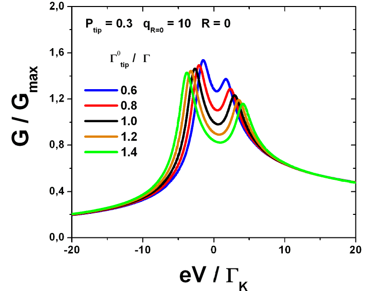
Not only the lateral tip-adatom separation can change the spin splitting, but also the vertical tip-adatom distance. To mimic this effect we change the ratio , thus introducing an asymmetry between the tip-adatom () and adatom-host () tunneling rates. When the tip becomes vertically closer to the adatom, we expect the increase of the coupling parameter . Consequently, the splitting between the peaks becomes more apparent (see figure (3)) which can be understood as consequence of the enhancement of the local tip magnetic field on the adatom due to the tip proximity.

4.2 Small tip-adatom coupling ()
In the small coupling limit the conductance curves (figure (4)) display dips instead of peaks observed in the large coupling limit (figures (2)-(3)). The appearance of the dips at is a consequence of a destructive quantum interference between the channels tip-host and tip-adatom-host. This can be easily seen from equations (24)-(25) for and that the LDOS behaves as
| (30) |
which is opposite to the case , where
| (31) |
As in the case of large coupling, the increase of the tip-adatom distance leads to a quenching of the anti-resonance splitting as it can be seen comparing the curves corresponding to different values of at figure (4). At Å, the asymmetric zero-bias anomaly for the dips disappears and only the standard single anti-resonance profile is recovered. A single dip structure in the conductance for small is verified for a system composed of Co on Cu(111) surface [19, 21]. It is valid to note that while the large limit resembles the embedded geometry, the small limit gives similar results to the T-shaped quantum dot (side-coupled geometry) [3, 42, 43].
4.3 Intermediate tip-adatom coupling ()
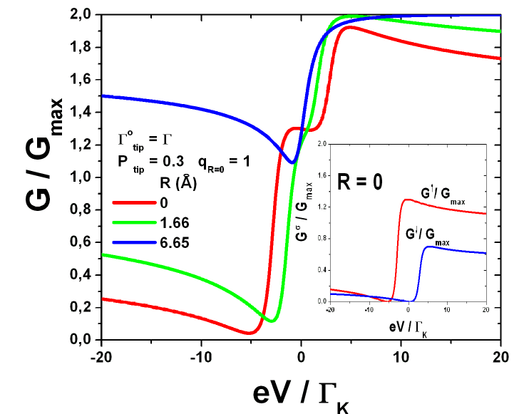
The intermediate case for a normal tip is characterized by the well known Fano-Kondo line shape [18, 21]. However, the introduction of a ferromagnetic tip results in distinct Fano-Kondo profiles for each spin component. The spin up profile is shifted toward negative bias with an enhanced amplitude, while the spin down case moves in the opposite direction being reduced in amplitude. This is illustrated in the inset of figure (5), where we show and .
The superposition of the spin-dependent Fano-Kondo profiles gives rise to the appearance of a plateau around the Fermi level () in the total conductance () for (see figure (5)). For large (Å), this plateau vanishes due to the suppression of the adatom’s Zeeman splitting and standard Fano-Kondo results for the conductance with nonmagnetic tips are recovered [18, 21].
5 Conclusions
We derived a spin resolved tunneling conductance for a system of a spin polarized STM tip with a single Kondo adatom on the surface of a normal metallic host. The conductance dependence on the tip bias was investigated for different tip-adatom lateral distances in a wide range of the Fano parameter , relevant for various experimental configurations. We demonstrated that the Fano parameter drastically affects the conductance pattern of the system. For large values of , we observe an asymmetric splitting of the Kondo resonance which is suppressed with an increase of the tip-adatom lateral distance. For small q, the behavior of the conductance is opposite to those observed in the large regime- instead of a splitted Kondo peak, one observes an asymmetrically splitted Kondo dip. For the intermediate case we have shown that due to the splitting of the spin resolved conductances (), the total conductance exhibits a plateau in the region of small biases, which disappears for large enough values of a tip-adatom lateral distance.
6 Acknowledgments
We thank L. N. Oliveira and M. Yoshida for stimulating discussions. This work was supported by the Brazilian agencies IBEM and CAPES.
References
References
- [1] Hewson A C, 1993 The Kondo Problem to Heavy Fermions (Cambridge University Press, Cambridge)
- [2] Goldhaber-Gordon D, Shtrikman H, Mahalu D, Abusch-Magder D, Meirav U and Kastner M A 1998 Nature 391 156
- [3] Sato M, Aikawa H, Sano A, Katsumoto S and Yie Y 2005 Phys. Rev. Lett. 95 066801
- [4] Busser C A, Moreo A and Dagotto E 2004 Phys. Rev. B 70 035402
- [5] Lobos A M and Aligia A A 2006 Phys. Rev. B 74 165417
- [6] Sfigakis F, Ford C J, Pepper M, Kataoka M, Ritchie D A and Simmons M Y 2008 Phys. Rev. Lett. 100 026807
- [7] Tripathi V and Cooper N R 2008 J. Phys: Condens. Matter 20 164215
- [8] For a review on spintronics see Zutic I, Fabian J, and Das Sarma S 2004 Rev. Mod. Phys. 76 323
- [9] Zhang P, Xue Q K, Wang Y and Xie X C 2002 Phys. Rev. Lett. 89 286803
- [10] Martinek J, Sindel M, Borda L, Barnaś J, König J, Schön G and von Delft J 2003 Phys. Rev. Lett. 91 247202
- [11] Martinek J, Utsumi Y, Imamura H, Barnaś J, Maekawa S, König J and Schön G 2003 Phys. Rev. Lett. 91 127203
- [12] Mahn-Soo Choi, Sánchez D and López R 2004 Phys. Rev. Lett. 92 056601
- [13] Martinek J, Sindel M, Borda L, Barnaś J, Bulla R, König J, Schön G, Maekawa S and von Delft J 2005 Phys. Rev. B 72 121302(R)
- [14] Utsumi Y, Martinek J, Schön G, Imamura H and Maekawa S 2005 Phys. Rev. B 71 245116
- [15] Świrkowicz R, Wilczyński M, Wawrzyniak M and Barnaś J 2006 Phys. Rev. B 73 193312
- [16] Hamaya K, Kitabatake M, Shibata K, Jung M, Kawamura M, Hirakawa K, Machida T and Taniyama T 2007 Appl. Phys. Lett. 91 232105
- [17] Pasupathy A N, Bialczak R C, Martinek J, Grose J E, Donev L A K, McEuen P L and Ralph D C 2004 Science 306 86
- [18] Madhavan V, Chen W, Jamneala T, Crommie M F and Wingreen N S 1998 Science 280 567
- [19] Manoharan H C, Lutz C P and Eigler D M 2000 Nature 403 512
- [20] Madhavan V, Chen W, Jamneala T and Crommie F 2001 Phys. Rev. B 64 165412
- [21] Knorr N, Alexander Schneider M, Lars Diekhöner, Peter Wahl and Klaus Kern 2002 Phys. Rev. Lett. 88 096804
- [22] Wahl P, Diekhöner L, Wittich G, Vitali L, Scheneider M A and K. Kern 2005 Phys. Rev. Lett. 95 166601
- [23] Ying-Shuang Fu, Shuai-Hua Ji, Xi Chen, Xu-Cun Ma, Rui Wu, Chen-Chen Wang, Wen-Hui Duan, Xia-Hui Qiu, Bon Sun, Ping Zhang, Jing-Feng Jia and Qin-Kue Xue 2007 Phys. Rev. Lett. 99 256601
- [24] Aguiar-Hualde J M, Chiappe G, Louis E and Anda E V 2007 Phys. Rev. B 76 155427
- [25] Chiappe G and Louis E 2006 Phys. Rev. Lett. 97 076806
- [26] Újsághy O, Kroha J, Szunyogh L and Zawadowski A 2000 Phys. Rev. Lett. 85 2557
- [27] Patton K R, Kettemann S, Zhuravlev A and Lichtenstein A 2007 Phys. Rev. B 76 100408(R)
- [28] The Fano parameter gives the strength of the quantum interference between different tunneling paths. It is proportional to the ratio between the tip-adatom and tip-host hopping coefficients
- [29] Fano U 1961 Phys. Rev. 124 1866.
- [30] Shelykh I A, Galkin N G 2005 Phys. Rev. B bf 70 05328
- [31] Shelykh I A, Galkin N G, Bagraev N T 2006 Phys. Rev. B 74 165331
- [32] Moldoveanu V, Tolea M, Gudmundsson V and Manolescu A 2005 Phys. Rev. B 72 085338
- [33] Frota H O and Oliveira L N 1986 Phys. Rev. B 33 7871
- [34] Frota H O 1992 Phys. Rev. B 45 1096
- [35] Silver R N, Gubernatis J E, Sivia D S and Jarrell M 1990 Phys. Rev. Lett. 65 496
- [36] Anderson P W 1961 Phys. Rev. 124 41
- [37] The Kondo temperature is calculated according to equation (24) of Costi T A, Hewson A C and Zlatić V 1994 J. Phys.: Condens. Matter 6 2519,
- [38] Schiller A and Hershfield S 2000, Phys. Rev. B 61 9036
- [39] Plihal M and Gadzuk J W 2001 Phys. Rev. B 63 085404
- [40] We note that in reference [27] the splitting depends on and not on the sum of as it was proposed in reference [11]. In our analysis we use the proposal of reference [11].
- [41] In the nonequilibrium regime, a system of a quantum dot coupled to a left and to a right normal electrodes exhibites two Kondo resonances pinned at the Fermi levels of the leads. See Krawiec M and Wysokiński K I 2002 Phys. Rev. B 66 165408. The influence of ferromagnetic leads on this nonequilibrium Kondo effect was studied in reference [11].
- [42] Seridonio A C, Yoshida M and Oliveira L N Preprint cond-mat/0701529
- [43] Lee W R, Kim J U and Sim H S 2008 Phys. Rev. B 77 033305