Traveling waves and Compactons in Phase Oscillator Lattices

Abstract

We study waves in a chain of dispersively coupled phase oscillators. Two approaches – a quasi-continuous approximation and an iterative numerical solution of the lattice equation – allow us to characterize different types of traveling waves: compactons, kovatons, solitary waves with exponential tails as well as a novel type of semi-compact waves that are compact from one side. Stability of these waves is studied using numerical simulations of the initial value problem.

I Introduction

The topic of this paper unifies two principal directions of nonlinear science: coupled self-sustained oscillators and soliton theory. Coupled autonomous self-sustained oscillators appear in different fields of science, they demonstrate a variety of fascinating phenomena. In this study we demonstrate that particularities of the coupling for a rather simple setup – all oscillators are identical, periodic, and form a regular lattice with a nearest neighbor coupling – can lead to highly nontrivial wave structures. Remarkably, a dispersive coupling of the phases of dissipative oscillators results in a simple lattice equation which is equivalent to a Hamiltonian one. We show that different types of traveling waves exist in this lattice: compactons (ultra-localized waves with a compact support), usual solitary waves with exponential tails, as well as the corresponding kink-type solutions. These waves appear from rather general initial conditions and exist for long times. After very long transients they are destroyed due to inelastic collisions and evolve into phase chaos.

Coupled autonomous oscillators are subject of high interest in nonlinear science Glass-01 ; Pikovsky-Rosenblum-Kurths-01 . When the coupling of the oscillators is weak, they can be described in the phase approximation Kuramoto-84 , where only a variation of the oscillator phases matters. The corresponding models are used for the description of lattices Ermentrout-Kopell-84 ; Kopell-Ermentrout-86 ; Sakaguchi-Shinomoto-Kuramoto-88 ; Ren-Ermentrout-00 ; Topaj-Pikovsky-02 , globally coupled ensembles and networks Kuramoto-84 ; Kuramoto-75 ; Daido-92a ; Daido-92 ; Strogatz-00 . In the absence of coupling, the phase equations have only zero Lyapunov exponents, therefore whether the phase dynamics is dissipative or conservative depends solely on the properties of the coupling. In studies which focus on synchronization properties, one typically assumes that the coupling is dissipative which thus tends to equalize the phases. However, certain types of coupling lead to a conservative dynamics – a prominent example is a splay state in a globally coupled ensemble of oscillators Tsang91 ; Nichols-Wiesenfeld-92 ; Strogatz-Mirollo-93 ; Watanabe-Strogatz-93 ; Watanabe-Strogatz-94 .

In the present work we consider the dynamics of a one-dimensional lattice of oscillators with a dispersive, conservative coupling. A realization of such a lattice may be a multi-core fiber laser Wrage_etal-00 , where individual self-oscillating lasers are arranged in a ring, or an array of Josephson junctions. Since both, the local phase dynamics and the coupling are non-dissipative, the dynamics is expected to be similar to that of the well-known Hamiltonian type. An example of a Hamiltonian lattice is the sine-Gordon lattice, for which the basic building blocks are traveling solitary waves like pulses or kinks, that on integrable lattices collide elastically, and in the non-integrable cases evolve into chaos Scott-99 .

In recent years two new concepts appeared that have significantly extended our understanding of nonlinear regimes in Hamiltonian lattices. One concept introduces localized periodic breathers Flach-Willis-98 ; the other introduces compact excitations in genuinely nonlinear lattices and wave equations. Unlike the usual solitons that have exponential, or algebraic, tails, the corresponding traveling waves have compact or almost compact support. These waves, named compactons, have been introduced in Rosenau-Hyman-93 ; Rosenau-94 ; Nesterenko-83 .

In the present paper we study general traveling waves in a chain of dispersively coupled nonlinear self-sustained oscillators, continuing our previous works Rosenau-Pikovsky-05 ; Pikovsky-Rosenau-06 focused on compacton solutions in phase oscillator chains. Contrary to Rosenau-Pikovsky-05 ; Pikovsky-Rosenau-06 , we consider here a generic phase model without additional symmetries. We show that dispersively coupled oscillators possess not only compactons, but also “classical” solitary waves with exponential tails. In dependence on parameters of the coupling and on the velocity these solution bifurcate. Remarkably, some of the compact solutions described in Rosenau-Pikovsky-05 ; Pikovsky-Rosenau-06 exist only in the symmetric situation, while other can be continued to the non-symmetric case. In the general, non-symmetric case, we describe a novel type of semi-compact waves which are compact from only one side and have an exponential tail on the other side. Another novel feature appears in the analysis of traveling waves on the lattice: here we describe a particular bifurcation from monotonic to oscillatory tails of a solitary wave, such a bifurcation does not exist in the quasicontinuous approximation where waves are described by means of a partial differential equation. We also report on a remarkable property of the solitary waves with exponential tails: they are extremely stable to collisions, so that a chaotization in a finite lattice occurs – contrary to the case of compactons – after exponentially long transients.

II Basic model

We consider the phase dynamics of a chain of identical self-sustained oscillators with frequency $\omega$

$$\frac{\mbox{d}\varphi_{n}}{\mbox{d}t}=\omega+q(\varphi_{n-1}-\varphi_{n})+q(\varphi_{n+1}-\varphi_{n})\text{.}$$ (1)

Here $\varphi_{n}$ is the phase of the $n$-th oscillator and $q(\varphi)=q(\varphi+2\pi)$ is the coupling function. Hereafter, we assume that this function is even, what corresponds to dispersive coupling, see Pikovsky-Rosenau-06 for details. Introducing the phase differences $v_{n}=\varphi_{n+1}-\varphi_{n}$ equation (1) can be rewritten as

$$\frac{\mbox{d}v_{n}}{\mbox{d}t}=\nabla_{d}q(v)=q(v_{n+1})-q(v_{n-1})\text{.}$$ (2)

The simplest possible even $2\pi$-periodic coupling function is $q(v)=\cos v$; this case was studied in Pikovsky-Rosenau-06 , where it was shown, that compactons and kovatons (glued together compact kink-antikink pairs) are solutions arising out of the background $v^{*}=0$. Here, we extend the results of Pikovsky-Rosenau-06 and demonstrate that this lattice also bears periodic waves and solitons, as well as semi-compact waves. In Pikovsky-Rosenau-06 it was also shown, that Eq. (2) is a Hamiltonian system. It possesses several integrals but is non-integrable. Additional symmetries in $q(v)$ may result in additional symmetries in Eq. (2), we will encounter them below.

Our main analytic tool for the study of the wave solutions of (2) is the quasi-continuous approximation (QCA). Associating $n$ with a continuous variable $x$, one develops $q(v_{n\pm 1})$ by the Taylor series expansion up to the third order

$$q(v_{n\pm 1})=\left[1\pm\frac{\partial}{\partial x}+\frac{1}{2}\frac{\partial^{2}}{\partial x^{2}}\pm\frac{1}{6}\frac{\partial^{3}}{\partial x^{3}}\right]q(v)\text{.}$$ (3)

Inserting this into (2) results in the partial differential equation

$$\frac{\partial v}{\partial t}=2\left[\frac{\partial}{\partial x}+\frac{1}{6}\frac{\partial^{3}}{\partial x^{3}}\right]q(v)\text{,}$$ (4)

which is the QCA for the lattice. We stress here, that this approximation is not based on a small parameter: because spacing between the sites is one, the higher-order terms are in general of the same order as the lower-order ones. Thus the validity of this approximation may be supported only by a comparison of its predictions (Section III) with the numerical solutions of the full equations (2) (Section IV).

III Traveling waves in the quasi-continuum

In this section we analyze waves in the QCA (4). First, we note that any constant $v=v^{*}$ is a solution. We will look for waves on the base of such a flat profile. Inserting the traveling wave ansatz $v(x,t)=v(x-\lambda t)=v(s)$, where $\lambda$ is the wave velocity, into Eq. (4) and integrating once yields

$$\lambda(v-v^{*})+2(q(v)-q(v^{*}))+\frac{1}{3}\frac{\mbox{d}^{2}}{\mbox{d}s^{2}}q(v)=0\text{.}$$ (5)

The integration starts at $s_{0}$, where it is assumed, that $v(s_{0})=v^{*}=\text{const}$. This is not valid for periodic waves, where one has to introduce the curvature of $q(v(s_{0}))$; however the resulting equations are equivalent to those derived below. We multiply Eq. (5) with $\displaystyle{{\mbox{d}q(v)}/{\mbox{d}s}}$ and integrate again, to obtain

$$\lambda\Big{[}q(v)\big{(}v-v^{*}\big{)}-Q(v,v^{*})\Big{]}+\big{(}q(v)-q(v^{*})\big{)}^{2}+\frac{1}{6}\left[\frac{\mbox{d}q}{\mbox{d}s}\right]^{2}=0\text{.}$$ (6)

The function $Q(v,v^{*})$ is defined as

$$Q(v,u)=\int_{u}^{v}q(x)\mbox{d}x$$ (7)

Equation (6) can be rewritten as

$$\left(\frac{\mbox{d}q}{\mbox{d}v}\right)^{2}\Bigg{[}\frac{1}{2}\left(\frac{\mbox{d}v}{\mbox{d}s}\right)^{2}+U(v)\Bigg{]}=0\text{,}$$ (8)

with the potential

$$U(v)=3\frac{\lambda[q(v)(v-v^{*})-Q(v,v^{*})]+\big{(}q(v)-q(v^{*})\big{)}^{2}}{(q^{\prime}(v))^{2}}\text{.}$$ (9)

Besides Eq. (8) one can also derive a system of first-order ODEs from Eq. (5), which reads

$$\frac{\mbox{d}v}{\mbox{d}s}=u\quad\text{,}\quad\frac{\mbox{d}u}{\mbox{d}s}=-\frac{3\lambda(v-v^{*})+6\big{(}q(v)-q(v^{*})\big{)}+q^{\prime\prime}(v)u^{2}}{q^{\prime}(v)}\text{.}$$ (10)

In the following we also need the properties of the linear approximation $q(v)=q(v^{*})+q^{\prime}(v^{*})(v-v^{*})$, then the equations (10) simplify to

$$\frac{\mbox{d}v}{\mbox{d}s}=u\quad\text{,}\quad\frac{\mbox{d}u}{\mbox{d}s}=-\frac{3\lambda+6q^{\prime}(v^{*})}{q^{\prime}(v^{*})}(v-v^{*})\text{,}$$ (11)

provided that $q^{\prime}(v^{*})\neq 0$. The stability of the fixed point at $v=v^{*}$ is determined by the eigenvalues of the Jacobian

$$l_{1,2}=\pm\sqrt{-(3\lambda+6q^{\prime}(v^{*}))/q^{\prime}(v^{*})}.$$ (12)

III.1 Solitary waves

Solitary waves on the base of the constant field $v=v^{*}$ are the homoclinic orbits of Eq. (8) and Eq. (10). They start at $v^{*}$, grow to a peak at $v_{m}$, and then go back to their origin $v^{*}$. An equation for the wave velocity $\lambda_{S}$ can be obtained from the condition $U(v_{m})=0$ which immediately yields

$$\lambda_{S}=\frac{\big{(}q(v_{m})-q(v^{*})\big{)}^{2}}{Q(v_{m},v^{*})-q(v_{m})(v_{m}-v^{*})}\text{.}$$ (13)

Solitary waves with exponential tails.

For the existence of a homoclinic trajectory one needs the fixed point of Eq. (10) to have one stable and one unstable direction, hence $v^{*}$ has to fulfill

$$-\frac{3\lambda+6q^{\prime}(v^{*})}{q^{\prime}(v^{*})}>0\text{.}$$ (14)

This condition yields a critical velocity $\lambda_{C}=-2q^{\prime}(v)$, which separates a saddle-type stationary solution from a center.

A solitary wave with exponential tails is shown in Fig. 4 below. The coupling function is $q(v)=\cos(v)$ and the background is $v^{*}=\pi/4$. The wave velocity is a free parameter, but bounded by the above condition. For the case $v^{*}=\pi/4$ and $v_{m}>v^{*}$ this results in $\lambda>2\sin\pi/4=\sqrt{2}$. In Fig. 4 the wave velocity was chosen to $\lambda=\pi/2$. The tails of the solitary wave decay exponentially, corresponding to the eigenvalues of the stationary state $v^{*}$.

Solitary waves with compact tails – Compactons.

Compactification may occur, if $q^{\prime}(v^{*})=0$. Linear waves do not exist around this point and the approximation in Eq. (11) does not hold. Therefore, one needs to approximate $q(v)$ to the second order in the vicinity of $v^{*}$. When this approximation is inserted into Eq. (4) one obtains the $K(2,2)$ equation, defined in Rosenau-Hyman-93 . For $q(v)\approx q(v^{*})+av^{2}$ a solution of (5) is given by

$$v(s)+v^{*}=\begin{cases}-\frac{2\lambda}{3a}\cos^{2}\left(\sqrt{\frac{3}{8}}s\right)&|x|<\pi\sqrt{\frac{2}{3}}\\ 0&\text{else.}\end{cases}$$ (15)

Usually, one cannot match two different solutions of one ODE, but here, the highest order operator degenerates at $v=v^{*}$ and the solutions uniqueness is lost. In the surrounding of $v^{*}$ the solution will behave like the $K(2,2)$ and compact waves occur in the full phase equation (4). In Fig. 5 below we show a compacton for the coupling function $q(v)=\cos v$ and $v^{*}=0$. The wave velocity was chosen to $\lambda=2/\pi$.

III.2 Kinks

The second class of traveling wave solutions are kinks, which correspond to heteroclinic orbits between two uniform states $v^{*}$ and $\bar{v}^{*}$. The height $\bar{v}^{*}$ of the kink has to fulfill condition (13) and furthermore it has to be a fixed point of (8), meaning that $U^{\prime}(\bar{v}^{*})=0$. This gives the following condition for the speed of the kink (it can also be derived from (5) where one assumes a constant solution $v_{m}=\text{const}$):

$$\lambda_{K}=2\frac{q(\bar{v}^{*})-q(v^{*})}{v^{*}-\bar{v}^{*}}\text{.}$$ (16)

Combining the velocity relations (13) and (16) by $\lambda_{S}=\lambda_{K}$ results in the final condition for the height of the kink

$$Q(\bar{v}^{*},v^{*})=\frac{(q(\bar{v}^{*})+q(v^{*}))(\bar{v}^{*}-v^{*})}{2}\text{.}$$ (17)

In Fig. 1 the values of possible uniform states connected by a kink are shown for the particular coupling function $q(v)=\cos v+a\cos 2v$. Note, that a bifurcation occurs at $a=\pm 1/4$ and two new branches of kink points emerge.

Figure 1: The values of uniform background states that can be connected by kinks, in the QCA for the particular coupling $q(v)=\cos v+a\cos 2v$ and various values of $a$.

For $q(v)=\cos v$ one finds $\bar{v}^{*}=\pi-v^{*}$ and the velocity belonging to this kink is $\lambda_{max}=\lambda_{K}=4\cos v^{*}/(\pi-2v^{*})$.

Kinks with exponential tails.

For kinks with exponential tails the same condition (14) as for the solitary waves has to be fulfilled. In Fig. 6 a kink with exponential tails is shown. The coupling function is $q(v)=\cos(v)$ and $v^{*}=\pi/4$, $\bar{v}^{*}=3\pi/4$. The velocity is $\lambda=\sqrt{32}/\pi$.

Compact kinks – Kovatons.

If $v^{*}$ and $\bar{v}^{*}$ fulfill the compactification condition $q^{\prime}(v^{*})=q^{\prime}(\bar{v}^{*})=0$, both tails will become compact and may form a compact kink-antikink pair, named kovaton Rosenau-Pikovsky-05 . An example of this wave form is shown in Fig. 7, with $q(v)=\cos v$ and $v^{*}=0$, $\bar{v}^{*}=\pi$ and $\lambda_{K}=4/\pi$.

Exponential-compact kinks.

In addition to kinks with exponential tails and kinks with compacton tails one can also observe semicompact kinks with one exponential and one compact tail. Consider the coupling $q(v)=\cos v+a\cos 2v$ with $a=0.2$. In this special setup $v^{*}=0$ fulfills the compactification condition and $\bar{v}^{*}=2.39955$ is the kink point satisfying (17) with velocity (16) $\lambda_{K}=1.60011$. This kink is shown in Fig. 8. It is compact at $v=v^{*}$ and exponential at $v=\bar{v}^{*}$.

III.3 Periodic waves

Periodic waves around $v^{*}$ exist if the eigenvalues $l_{1,2}$ in (12) are purely imaginary. A periodic wave in the QCA is shown in Fig. 9. The velocity of a periodic wave must satisfy the condition resulting from (10):

$$-\frac{3\lambda+6q^{\prime}(v^{*})}{q^{\prime}(v^{*})}<0\text{.}$$ (18)

For $q(v)=\cos v$ and $0<v^{*}<\pi$ this condition yields $\lambda<2\sin v^{*}$. At $\lambda=\lambda_{C}=-2q^{\prime}(v^{*})$ some kind of bifurcation occurs.

To quantify the dynamical behavior of the QCA near $\lambda_{C}$ we simplify (10) to

$$\frac{\mbox{d}v}{\mbox{d}s}=u\quad\text{,}\quad\frac{\mbox{d}u}{\mbox{d}s}=\lambda(v-v^{*})-v^{2}-{v^{*}}^{2}\text{.}$$ (19)

This ODE is not an approximation of (10) in a strict sense, since we have neglected the terms $q^{\prime\prime}(v)u^{2}$ and $q^{\prime}(v)$, but the qualitative behavior does not change. System (19) has two fixed points $(v_{1},u_{1})=(v^{*},0)$ and $(v_{2},u_{2})=(\lambda-v^{*},0)$. The eigenvalues of the corresponding Jacobian are

$$l_{1,2}^{(1)}=\pm\sqrt{\lambda-2v^{*}}\;\qquad l_{1,2}^{(2)}=\pm\sqrt{2v^{*}-\lambda}\text{.}$$

If the velocity reaches the critical value $\lambda_{C}=2v^{*}$, the two fixed points coincide and furthermore both fixed points change their roles; if $\lambda<\lambda_{C}$ the center is $(v_{1},u_{1})$ and $(v_{2},u_{2})$ is a saddle-point; if $\lambda>\lambda_{C}$ the roles have changed and $(v_{1},u_{1})$ is the saddle and $(v_{2},u_{2})$ is the center. Now we return to Eq. (10). In Fig. 2 the phase space of (10) near the critical velocity is shown. If $\lambda<\lambda_{C}$ the first fixed point will be a center, hence periodic waves exists in the QCA and for $\lambda>\lambda_{C}$ the fixed point is a saddle point. Furthermore, the unstable and the stable manifold of this saddle are connected – a homoclinic orbit exists, resulting in solitonic solutions in the QCA. So, at the critical velocity we have a transition or a bifurcation from periodic waves to solitons.

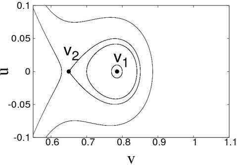
(a) $\lambda=\lambda_{S,min}-0.1$

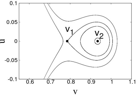
(b) $\lambda=\lambda_{S,min}+0.1$

Figure 2: Phase space of (10) for $v^{*}=\pi/4$ and a) $\lambda=\lambda_{C}-0.1$ and b) $\lambda=\lambda_{C}+0.1$. The critical velocity is $\lambda_{C}=2\sin\pi/4=\sqrt{2}$. It is clearly visible that below the critical velocity the fixed point $(v_{1},u_{1})$ is a center, hence periodic waves exist in (4). Above $\lambda_{C}$ one can observe solitonic solutions: the background $v_{1}$ is a saddle point and a homoclinic orbit exists.

IV Traveling waves in the lattice

Now we turn our attention to traveling waves in the full phase lattice model (2). The wave ansatz for this model can be formulated as

$$v_{n}(t)=v(n-\lambda t)=v(s)$$ (20)

with velocity $\lambda$. Inserting (20) into (2) yields

$$\dot{v}=\frac{1}{\lambda}\Big{(}q\big{(}v(s-1)\big{)}-q\big{(}v(s+1)\big{)}\Big{)}\text{.}$$ (21)

We integrate this equation from $s_{0}$ to $s$ to obtain

$$v(s)-v^{*}=\frac{1}{\lambda}\int_{s-1}^{s+1}\big{[}q(v^{*})-q(v(\tau))\big{]}\mbox{d}\tau\text{,}$$ (22)

where it is supposed, that $v(s<s_{0})=v^{*}$. Again, as in the continuous version, the exact initial conditions $v(s_{0})$ are not relevant, they can be absorbed into the constant of integration. If one requires that $v(s)=\bar{v}^{*}$ is a constant solution, hence a kink exist, the corresponding velocity $\lambda_{K}$ has to satisfy

$$\lambda_{K}=2\frac{q(v^{*})-q(\bar{v}^{*})}{\bar{v}^{*}-v^{*}}\text{.}$$ (23)

This condition is exactly analogous to condition (16) in the QCA.

IV.1 Fixed point analysis

Similar to the fixed point analysis in the QCA, one can analyze the behavior of traveling waves close to the background $v^{*}$. To this end we linearize $q(v)\approx q(v^{*})+a(v-v^{*})$ in (21) and apply the exponential ansatz $v(t)=A\exp lt$. This yields the characteristic equation

$$l=\frac{a}{\lambda}(e^{-l}-e^{l})\text{.}$$ (24)

Note again, that $a=q^{\prime}(v^{*})\neq 0$, meaning that this approximation does not hold for the compacton backgrounds.

We split $l$ into its real and imaginary part $l=p+\text{i}q$ to obtain

$$p=-2\frac{a}{\lambda}\cos q\sinh p\qquad\text{and}\quad q=2\frac{a}{\lambda}\sin q\cosh p\text{.}$$ (25)

For a purely imaginary eigenvalues $p=0$ we obtain

$$q=-2\frac{a}{\lambda}\sin q\quad\text{or}\quad\lambda=-2a\frac{\sin q}{q}\text{.}$$ (26)

This function is plotted in Fig. 3(a). In this plot, the dots mark possible points for transitions to eigenvalues with real parts. In Fig. 3(b) all eigenvalues $l=p+\text{i}q$ are shown. Purely real eigenvalues are

$$p=-2\frac{a}{\lambda}\sinh p\quad\text{or}\quad\lambda=-2a\frac{\sinh p}{p}\text{.}$$ (27)

So, when $\lambda$ crosses $-2a$ (point 1 in Fig. 3(a)), a bifurcation from two purely imaginary eigenvalues to two purely real eigenvalues occurs. This scenario corresponds to the transition from periodic to solitary waves and the critical velocity is $\lambda_{C}=-2a$. The situation is analogous to the bifurcation in the QCA and the critical velocity is the in both situations.

The next bifurcation occurs, when $\lambda$ crosses point 2, see Fig. 3. Then, a bifurcation from a center to a stable and an unstable spiral point occurs. This refers to the transition from periodic waves to solitary waves with oscillating tails and exponentially decaying amplitude. Since the bifurcation occurs on the imaginary axis, one can calculate the critical velocity from (25) by setting $\lambda^{\prime}(q)=0$ and for the special case $q(v)=\cos v$ one obtains $\lambda\approx-2a\cdot 0.217$. Note, that there is no counterpart in the QCA for this bifurcation.

(a) (b)

Figure 3: (a): Wave speed $\lambda$ in dependence of the imaginary eigenvalue $q$, see (26). The dots mark possible bifurcation points to real eigenvalues. (b): Wave speed $\lambda$ vs. the real and imaginary part of the eigenvalues, with $a=\sin(0.2)$. Only the positive parts of the real and imaginary axes are shown.

IV.2 Numerical determination of traveling waves

From (22) it is possible to construct a numerical scheme to find solitary wave solutions of the lattice Pikovsky-Rosenau-06 ; Petviashvili-76 ; Petviashvili-81 . One initially guesses a wave profile $v_{0}(t)$ and than iterates

$$\tilde{v}(s)=v^{*}+\frac{1}{\lambda}\int_{s-1}^{s+1}\big{(}q(v^{*})-q(v_{k}(\tau))\big{)}\mbox{d}\tau\qquad v_{k+1}=\left(\frac{||v_{k}||}{||\tilde{v}||}\right)^{3/2}\tilde{v}\text{,}$$ (28)

$||\cdot||$ denotes the $L_{1}$-norm. The integral is calculated by a high order Lagrangian integration rule Abramowitz-Stegun-64 . To construct kink solutions, one has to omit the normalization in (28) by setting $v_{k+1}=\tilde{v}$. Periodic waves can be obtained by a slight modification of (28). Here, the wave length $w$ is introduced and periodic boundary conditions $\tilde{v}(0)=\tilde{v}(w)$ are assumed in (28).

We want to point out two issues one has to keep in mind when using this algorithm. First, in (28) the normalization exponent $3/2$ is used. In a few cases this exponent is to large and has to be set to smaller values, otherwise the algorithm will diverge. Secondly, for backgrounds different from $0$ one has to shift the coordinates $v\mapsto v^{*}+v$.

IV.3 Solitary waves

Solitary waves arise out of a background with one stable and one unstable direction. So, they have to fulfill $(\lambda+2q^{\prime}(v^{*}))/q^{\prime}(v^{*})>0$ in order to obtain two real eigenvalues of the fixed point.

Solitary waves with exponential tails.

In Fig. 4 we show a solitary wave with exponential tails. The coupling is $q(v)=\cos v$ and the background is $v^{*}=\pi/4$. The velocity of was chosen to $\lambda=\pi/2$, fulfilling the condition $(\lambda+2q^{\prime}(v^{*}))/q^{\prime}(v^{*})>0$. The solitary wave was computed with the scheme (28).

Figure 4: Top panel: Soliton solution for the coupling $q(v)=\cos v$, which arise out of the background $v^{*}=\pi/4$. The form of the soliton was calculated numerically with the help of (28) and the velocity is $\lambda=\pi/2$. Here and in the following figures bold dots show the soliton on the lattice and the dashed line the solution of QCA (5) which has an additional offset for better visibility. Bottom panel: the soliton in logarithmic scale.

Compact solitary waves.

Again, as in the QCA, the condition $q^{\prime}(v^{*})=0$ allows the compactification of the tails. In Fig. 5 we show a compacton arising out of the background $v^{*}=0$ for the coupling $q(v)=\cos v$. The wave velocity was set here to $\lambda=2/\pi$. The compacton is not purely compact, but has super-exponentially decaying tails Pikovsky-Rosenau-06 . Thus, although there is a qualitative difference between the lattice and the QCA, quantitatively these solutions are very close to each other.

Figure 5: Top panel: the shape of the compacton for the coupling $q(v)=\cos v$. The background is $v^{*}=0$ and the velocity was set to $\lambda=2/\pi$. Markers show the compacton on the discrete lattice and the dashed line is the corresponding solution in the quasi-continuum approximation. Bottom panel: the same plot in logarithmic scale. The super exponentially decaying tails are clearly visible.

IV.4 Kinks

To derive an analogon to (17), we rewrite Eq. (23) as $\lambda_{K}\big{(}\bar{v}^{*}-v^{*}\big{)}=2\big{(}q(v^{*})-q(\bar{v}^{*})\big{)}$, multiply with $q^{\prime}(\bar{v}^{*})$, and integrate over $\bar{v}^{*}$ from $v^{*}$ to $\bar{v}^{*}$ to obtain

$$\lambda_{K}\int_{v^{*}}^{\bar{v}^{*}}q^{\prime}(v)\big{(}v-v^{*})\mbox{d}v=2\int_{v^{*}}^{\bar{v}^{*}}q^{\prime}(v)\Big{(}q(v^{*})-q(v)\Big{)}\mbox{d}v\text{,}$$ (29)

and finally

$$\lambda_{K}=\frac{\big{(}q(v^{*})-q(\bar{v}^{*})\big{)}^{2}}{Q(\bar{v}^{*},v^{*})-q(\bar{v}^{*})\big{(}\bar{v}^{*}-v^{*}\big{)}}\text{.}$$ (30)

Combining Eq. (23) and (30) yields

$$Q(\bar{v}^{*},v^{*})=\frac{(q(\bar{v}^{*})+q(v^{*}))(\bar{v}^{*}-v^{*})}{2}\text{,}$$ (31)

which matches exactly the kink condition for the QCA.

Kinks with exponential tails.

In Fig. 6 we show the shape of a kink. The coupling is $q(v)=\cos v$ and the background is $v^{*}=\pi/4$. The velocity of the kink is given by (23) $\lambda_{K}=\sqrt{32}/\pi$.

Figure 6: Top panel: The shape of the kink for $v^{*}=\pi/4$, the velocity is $\lambda=\sqrt{32}/\pi$. Center panel: The kink in logarithmic scale. Bottom panel: The kink shown from its top in logarithmic scale. Markers show the kink on the lattice and the dashed line is the QCA with an additional offset for better visibility.

Kinks with compact tails.

One can observe compact kinks, if $q^{\prime}(v^{*})=0$ and $q^{\prime}(\bar{v}^{*})=0$. For the coupling $q(v)=\cos v$ such a case exists with $v^{*}=0$ and $\bar{v}^{*}=\pi$. The shape of this compact kink is shown in Fig. 7. Here, the velocity is $\lambda=4/\pi$.

Figure 7: Top panel: The wave form of the compact kink solution between $v^{*}=0$ and $\bar{v}^{*}=\pi$ for the coupling $q(v)=\cos v$. Markers show the wave form on the discrete lattice and the dashed line represents the quasi-continuum approximation of the kink. Bottom panel: The sine of the kink in logarithmic scale.

Semi-compact kinks.

It also possible to observe kinks with one exponential decaying tail and one compact tail. This is the case for $q(v)=\cos v+a\cos 2v$ with $a=0.2$. For $\lambda=1.60011$ and $\bar{v}^{*}=2.39955$ the kink condition (31) is satisfied and such a kink is found by the numerical method described above, see Fig. 8.

Figure 8: Top panel: The shape of a kink with one exponential and one compact tail. The coupling for this specific wave is $q(v)=\cos v+a\cos 2v$ with $a=0.2$. The position of the kink point and the wave velocity can be obtained from (31) and (23), their values are $\lambda=1.60011$ and $\bar{v}^{*}=2.39955$. Middle panel: The kink in logarithmic scale. The compact tail of the kink is hear clearly visible. Bottom panel: The kink shown from its top in logarithmic scale, the exponential tail becomes visible.

IV.5 Periodic waves

Periodic waves can be calculated with (28) and periodic boundary conditions. An example is shown in Fig. 9. Here, the offset is $v^{*}=\pi/4$, the wave length is $w=5\pi$ and the velocity is $\lambda=\pi/2$.

Figure 9: The shape of a periodic wave on the lattice. The offset is $v^{*}=\pi/4$, the wave length is $w=5\pi$ and the velocity $\lambda=\pi/2$.

IV.6 Solitary waves with periodically decaying tails

From the fixed point analysis of the advanced-delayed equation (21) a bifurcation occurs at point 2 in Fig. 3(a). So, if the velocity $\lambda$ reaches the critical point $\lambda_{C}$, the fixed point changes its type from a center to a stable and an unstable focus. This corresponds to a solitary wave with oscillatory decaying tails. In Fig. 10 we show an example of such a wave. The offset is $v^{*}=-0.2$ and the wave velocity is $\lambda=1.0$. This behavior does not occur in the quasi continuum.

Figure 10: Solitary wave with periodic and exponentially decaying tails. $v^{*}=-0.2$ and $\lambda=1.0$. The plot was generated with the help of the traveling wave scheme (28) for the lattice equation; it has no QCA counterpart.

V Numerical simulations of the initial value problem

In this section we demonstrate, how the traveling waves described in the previous sections appear in the course of the evolution of the lattice. We will restrict ourselves to the simplest coupling term $q(v)=\cos v$, while the background state will be general $v^{*}\neq 0$. Furthermore, we will study the stability properties of the colliding waves.

V.1 Evolution of an initial pulse

First, we consider the evolution of an initial $\cos$-pulse with the coupling $q(v)=\cos v$. The initial condition is

$$v_{n}(0)=\begin{cases}v^{*}+\frac{A}{2}\left[1+\cos\left(\frac{n-n_{0}}{w}\pi\right)\right]&|n-n_{0}|<w\\ v^{*}&\text{else,}\end{cases}$$ (32)

where $A$ is the amplitude, $n_{0}$ is the center and $w$ is the half width of the pulse.

In Figs. 11,12 we compare the evolution for different values of $v^{*}$. In Fig. 11 we set $v^{*}=0$ ($q^{\prime}(v^{*})=0$) and one can observe compactons and kovatons arising from the initial pulse. In Fig. 11(a) a wave train of compactons emerges out of the initial pulse. The speed of the compactons increases with increasing amplitude. In Fig. 11(b) we have increased the width and the amplitude of the pulse and one kovaton is observed. In the bottom plot of Fig. 11 a narrow initial pulse creates a wave source, emitting periodic waves.

In Fig. 12 we show results for the background $v^{*}=\pi/4$. Here, $q^{\prime}(v^{*})\neq 0$ and the solitary waves arising from the initial pulse possess exponential tails. Fig. 12(a),(b) are similar to Fig 11(a),(b), where the initial pulse decomposes into a train of solitons and kink. Note, that the number of emitted solitary waves is smaller than for the case $v^{*}=0$. Furthermore, periodic waves around $v^{*}$ can emerge, see Fig. 12(c) and (d). The plot in (d) is somehow similar to Fig. 11(c), with the difference, that appearing periodic waves are around $v^{*}$. Fig. 12(e) shows the evolution of a narrow initial pulse with a relative large amplitude. It results in a kink with periodic waves around the top of the kink. A detailed analysis of all possible waveforms goes beyond the scope of this paper and will be reported elsewhere.

Figure 11: Evolution of different initial pulses for the coupling $q(v)=\cos v$ and $v^{*}=0$. The initial conditions were set according to (32). (a) $w=10$ and $A=2$, (b) $w=15$ and $A=3$ and (c) $w=1$ and $A=1$. The dashed line shows the initial condition $v_{n}(t=0)$ and the solid line the lattice at the time $t=100$.

Figure 12: Evolution of different initial pulses for the coupling $q(v)=\cos v$ and the background $v^{*}=\pi/4$. The initial conditions were set according to (32). (a) $w=10$ and $A=1$, (b) $w=15$ and $A=1.5$, (c) $w=10$ and $A=2$, (d) $w=1$ and $A=1$ and (e) $w=1$ and $A=2$. The dashed line shows the initial condition $v_{n}(t=0)$ and the solid line the lattice at the time $t=100$. Furthermore the position of the kink point at $3/4\pi$ is shown.

V.2 Transition to chaos in a finite lattice

Wave trains shown in Figs. 11,12 are obtain for an effectively infinite lattice (during the calculation times the boundaries are not reached). In a finite lattice, collisions between waves occur. We have used periodic boundary conditions, and observed that at large times eventually a chaotic regime appears. In Fig. 13 we show the evolution of an initial $\cos$ pulse with $v^{*}=0.1$. The upper plot shows the initial decomposition of this pulse into one kink and several solitary waves. These structures appear to survive collisions quite unaffected. The lower plot shows, that after some transient time chaos emerges. The chaotic state begins to develop, after a collision of two solitons produces a large-amplitude soliton-antisoliton pair. Then an avalanche of soliton-antisoliton collisions is triggered on, resulting in a fast chaotization.

In Fig. 14 we show a remarkable dependence on the average transient time, after which chaos establishes, on the parameter $v^{*}$. For larger values of $v^{*}$ the transient time is exponentially large, what means extreme stability of the solitary waves. Qualitatively, this stability can be attributed to a smallness of effects of discreteness of the lattice for large $v^{*}$. Here, the waves are relatively wide, thus they are well approximated in the QCA, which is close to the integrable Korteveg-de Vries equation. For small $v^{*}$ the waves are close to compactons that are short and for them the discreteness that causes non-elasticity of collisions is essential. Furthermore, the number of emitted waves decreases with increasing $v^{*}$ and the velocity of the waves is bounded from below. These two effects reduce the possibility that two waves meet each other, resulting in an increased transient time.

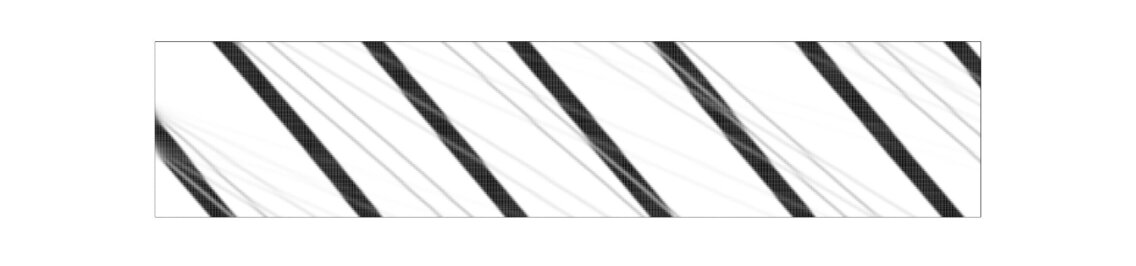
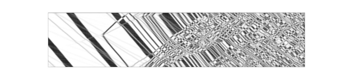
Figure 13: Transition to chaos. The background is $v^{*}=0.1$ and the lattice contains of $N=100$ sites with periodic boundary conditions. The field is shown in a gray scale versus time (horizontal axis) and space (vertical axis). Upper plot: A kink and several solitons emerge out of an $\cos$ pulse. The time interval is $0\leq t\leq 400$. Lower plot: Emergence of chaos after a collision of two solitons which creates an soliton-antisoliton pair. The time interval is $2600\leq t\leq 3000$.

Figure 14: Transient times to chaos for different backgrounds $v^{*}$. The length of the lattice is $N=32$ and the initial $\cos$-pulse is $v_{n}=\pi/4\big{(}\cos(\pi(n-N/2)/w)+1\big{)}+v^{*}$ for $|n-N/2|<w$ and $v=v^{*}$ else. In order to obtain an average of the transient times we also varied the width of the initial pulse from $5$ to $15$ and calculated the transient time as the average over the transient times for different initial pulses. The line is an exponential fit and the transient times scales with $T\sim\exp{16.7v^{*}}$.

VI Conclusions

We have demonstrated a variety of nontrivial wave structures in dispersively coupled oscillator lattices. Remarkably, they appear in a very simple lattice described by Eq. (2). In this study we have focused, contrary to previous works Rosenau-Pikovsky-05 ; Pikovsky-Rosenau-06 , on the features that appear for a general, non-symmetric coupling function. While some nontrivial solutions (compactons) survive in a general case, other (kovatons) exist only in the symmetric situation. Instead, for a general case we have reported a novel type of semi-compact waves. In our study of the waves on a lattice we have described a novel transition from monotonic to oscillatory tails of solitary waves that does not exist in the quasicontinuous approximation. Our comparison of general typical solutions of the lattice model with special ones studied in Rosenau-Pikovsky-05 ; Pikovsky-Rosenau-06 has shown that the waves with exponential tails are much more “resistant” to chaotization compared to the compactons.

Here, we would outline several possible extensions of the analysis. In general, coupling between oscillators can possess both dispersive and dissipative parts. The waves described in this work will still be observed if the dissipation is sufficiently small, this is confirmed by the perturbation analysis in Pikovsky-Rosenau-06 . Another feature disturbing the waves is a non-homogeneity of the lattice, e.g. due to non-uniformity of coupling. We expect that the waves will scatter on such inhomogeneities, but this issue has not been studied yet. Finally, it is intriguing, what kinds of waves can be observed in two- and three-dimensional lattices; results in this direction will be published elsewhere.

We thank P. Rosenau for helpful discussions and DFG for support.

References

- (1) L. Glass. Synchronization and rhythmic processes in physiology. Nature, 410:277–284, 2001.
- (2) A. Pikovsky, M. Rosenblum, and J. Kurths. Synchronization. A Universal Concept in Nonlinear Sciences. Cambridge University Press, Cambridge, 2001.
- (3) Y. Kuramoto. Chemical Oscillations, Waves and Turbulence. Springer, Berlin, 1984.
- (4) G. B. Ermentrout and N. Kopell. Frequency plateaus in a chain of weakly coupled oscillators, I. SIAM J. Math. Anal., 15(2):215–237, 1984.
- (5) N. Kopell and G. B. Ermentrout. Symmetry and phase locking in chains of weakly coupled oscillators. Comm. Pure Appl. Math., 39:623–660, 1986.
- (6) H. Sakaguchi, S. Shinomoto, and Y. Kuramoto. Mutual entrainment in oscillator lattices with nonvariational type interaction. Prog. Theor. Phys., 79(5):1069–1079, 1988.
- (7) L. Ren and B. Ermentrout. Phase locking in chains of multiple-coupled oscillators. Physica D, 143(1-4):56–73, 2000.
- (8) D. Topaj and A. Pikovsky. Reversibility versus synchronization in oscillator lattices. Physica D, 170(2):118–130, 2002.
- (9) Y. Kuramoto. Self-entrainment of a population of coupled nonlinear oscillators. In H. Araki, editor, International Symposium on Mathematical Problems in Theoretical Physics, page 420, New York, 1975. Springer Lecture Notes Phys., v. 39.
- (10) H. Daido. Order function and macroscopic mutual entrainment in uniformly coupled limit-cycle oscillators. Prog. Theor. Phys., 88(6):1213–1218, 1992.
- (11) H. Daido. Quasientrainment and slow relaxation in a population of oscillators with random and frustrated interactions. Phys. Rev. Lett., 68(7):1073–1076, 1992.
- (12) S. H. Strogatz. From Kuramoto to Crawford: Exploring the onset of synchronization in populations of coupled oscillators. Physica D, 143(1-4):1–20, 2000.
- (13) K. Y. Tsang, R. E. Mirollo, S. H. Strogatz, and K. Wiesenfeld. Dynamics of globally coupled oscillator array. Physica D, 48:102–112, 1991.
- (14) S. Nichols and K. Wiesenfeld. Ubiquitous neutral stability of splay-phase states. Phys. Rev. A, 45:8430–8435, 1992.
- (15) S. H. Strogatz and R. E. Mirollo. Splay states in globally coupled Josephson arrays: Analytical prediction of Floquet multipliers. Phys. Rev. E, 47(1):220–227, 1993.
- (16) S. Watanabe and S. H. Strogatz. Integrability of a globally coupled oscillator array. Phys. Rev. Lett., 70(16):2391–2394, 1993.
- (17) S. Watanabe and S. H. Strogatz. Constants of motion for superconducting Josephson arrays. Physica D, 74:197–253, 1994.
- (18) M. Wrage, P. Glas, D. Fischer, M. Leitner, D. V. Vysotsky, and A. P. Napartovich. Phase locking in a multicore fiber laser by means of a Talbot resonator. Optics Letters, 25(19):1436–1438, 2000.
- (19) A. Scott. Ninlinear science: emergence and dynamics of coherent structures. Oxford UP, Oxford, 1999.
- (20) S. Flach and C. R. Willis. Discrete breathers. Physics Reports, 295(5):181–264, 1998.
- (21) P. Rosenau and J. M. Hyman. Compactons: Solitons with finite wavelength. Phys. Rev. Lett., 70(5):564–567, 1993.
- (22) P. Rosenau. Nonlinear dispersion and compact structures. Phys. Rev. Lett., 73:1737–1741, 1994.
- (23) V. F. Nesterenko. Propagation of nonlinear compression pulses in granular media. J. Appl. Mech. Tech. Phys., 5:733–743, 1983.
- (24) P. Rosenau and A. Pikovsky. Phase compactons in chains of dispersively coupled oscillators. Phys. Rev. Lett., 94:174102, 2005.
- (25) A. Pikovsky and P. Rosenau. Phase compactons. Physica D, 218:56–69, 2006.
- (26) V. I. Petviashvili. Sov. J. Plasma Phys., 2:257, 1976.
- (27) V. I. Petviashvili. Multidimensional and dissipative solitons. Physica D, 3(1-2):329–334, 1981.
- (28) M. Abramowitz and I. A. Stegun. Handbook of Mathematical Functions. Department of Commerce USA, Washington, D.C., 1964.