The B3-VLA CSS sample.
VII: WSRT Polarisation Observations and the Ambient Faraday Medium Properties Revisited

We present new polarisation observations at 13 cm, acquired using the Westerbork Synthesis Radio Telescope (WSRT), of 65 sources, from the B3-VLA sample of Compact Steep-Spectrum sources. These new data are combined with our VLA polarisation data, at 3.6, 6 and, 21 cm, presented in a previous paper. Due to the multi-channel frequency capabilities of the WSRT, these new 13 cm observations enable a more reliable determination of integrated Rotation Measures, and of depolarisation behaviour with wavelength. The new data are inconsistent with the depolarisation models that we used earlier, and we propose an alternative model which seems to work properly. We also revise our previous model for the external Faraday screen, and its dependence on the source redshift.

1 Introduction

Compact Steep-Spectrum (CSS) sources and GHz-Peaked Spectrum (GPS) sources, because of their small size, are fully embedded in the Interstellar Medium (ISM) of the host galaxy. Their radio properties are affected by the properties of the ISM, unlike large-size radio sources which extend well beyond the optical dimensions of their host galaxies, and can therefore be used to probe the conditions of the ISM. Polarisation characteristics are a useful tool for this purpose.

The measurable quantities from polarisation observations are:

• The Faraday Rotation Measure (RM), defined as the slope of a linear fit of the polarisation angles, as a function of $\lambda^{2}$:

  $$\chi(\lambda)=RM\leavevmode\nobreak\ \lambda^{2}+\chi(0).$$

  If the medium is homogeneous (both its density and magnetic field), or if the inhomogeneities are resolved by the observing beam, $\chi(\lambda)$ is strictly proportional to $\lambda^{2}$ at all wavelengths, and $RM=k\int B_{||}nd\ell$ (this quantity is also called Faraday Depth), where $B_{||}$ is the component of the magnetic field along the line of sight, $n$ is the electron density of the medium, $\ell$ is the geometrical depth of the medium along the line of sight (los), and $k$ is a constant. If the medium is unresolved, or partially resolved by the observing beam, RM changes from point to point across the source, different contributions of polarised radiation are rotated differently, and $\chi(\lambda)$ can deviate, more or less strongly, from the $\lambda^{2}$-linear law.

• The change of the fractional polarisation $m{{}_{\lambda}}$ with $\lambda$, described by the quantity $DP(\lambda)=m_{\lambda}/m_{0}$. If the medium is uniform, or if its inhomogeneities are well resolved by the observing beam, $DP(\lambda)=1$. In an inhomogeneous medium, the variations of RM from point to point will produce changes in $m_{\lambda}$ versus $\lambda$. $DP(\lambda)$ will exhibit different behaviours with $\lambda$, depending on the properties of the inhomogeneities inside the medium.

Several models have been developed to interpret the Faraday effects (e.g.  Burn 1966; Tribble 1991; see also  Laing 1984 for an excellent and concise review). The behaviour of the polarisation angle, $\chi(\lambda)$, and fractional polarisation, $m_{\lambda}$, as a function of $\lambda^{2}$, enables the “average” Faraday Rotation Measure, and, from the “screen models”, its dispersion, $\sigma_{\rm RM}$, to be determined. Using these data, we can obtain information on the density distribution of the ISM that surrounds the radio source, on its clumpiness, and on both the ordered and tangled components of the magnetic field.

Polarisation studies of CSS and GPS source samples have been conducted by several authors  (e.g. van Breugel  et al. 1984; Akujor & Garrington 1995; Stanghellini  et al. 1998; Peck & Taylor 2000). They have found that GPS sources are almost unpolarised, while the larger-size CSS sources can show large RMs and/or large depolarisations, as a function of $\lambda^{2}$.

In a previous paper  (Fanti  et al. 2004, hereafter Paper IV), we used “low resolution” polarisation measures at 8.5 and 4.9 GHz ($\approx 3.6$ and 6 cm) from  Fanti  et al. (2001, hereafter Paper I), and at 1.4 GHz ($\approx 21$ cm) from the NVSS  (Condon  et al. 1998), to derive the RM and the depolarisation properties of a complete sample of CSSs, the B3-VLA CSS sample (Paper I). Our main results were:

1. In general, the total source depolarisation was found to follow either the Burn or the Tribble model.

2. In $\geq 50$% of the cases, the integrated $\chi(\lambda)$ follows the $\lambda^{2}$-linear law from 3.6 to 20 cm. The derived RMs have values of up to a few hundred rad m^-2. After subtraction of the Galactic Rotation, and correction for the source redshift, z, we found that $\approx 20$% of the sources have intrinsic $RM$s of up to 1000 rad m^-2.

3. There is a wavelength-dependent characteristic scale (from $\approx 3$ kpc at 3.6 cm to $\geq 6$ kpc at 21 cm), below which radio sources are almost totally depolarised  (see also Cotton  et al. 2003).

4. $\sigma_{\rm RM}$ increases with redshift; a similar, but less significant, dependence was suggested for RM (Figs. 13 and 14 in  Paper IV).

To explain our results, we proposed a simple model, based on Faraday effects, with an appropriate spatial distribution of the ambient gas density and magnetic field.

The results of  Paper IV, however, were based on polarisation data with a non-optimal wavelength coverage, because the gap in $\lambda^{2}$, between 6 and 20 cm, is too wide. In a number of cases there were remaining ambiguities in both RM and $\sigma_{\rm RM}$. In fact, for the few sources for which a polarisation measurement was available at the intermediate wavelength of 11  cm  (Klein  et al. 2003) the initial model was not supported in a number of cases (see Figs. 4 and 10 in  Paper IV).

To improve our polarisation information we performed new polarisation observations at 13 cm, using the Westerbork Synthesis Radio Telescope (WSRT) for 65 radio sources, 58 of which were detected in polarisation at one or more of the three available VLA frequencies. The remaining 7 unpolarised objects were observed as control sources.

The new observations fill the large gap in $\lambda^{2}$ between the 6 and 21 cm VLA data. They allow us to improve the reliability of the RMs significantly by reducing the ambiguities, and constrain the depolarisation behaviour as a function of $\lambda^{2}$.

Section 2 provides a short description of the B3-VLA CSS sample and of the previous polarisation data (3.6, 6, and 21 cm, VLA), and presents the selection criteria for the WSRT sub-sample.

Sections 3 describes the new WSRT polarisation observations at 13 cm, the data reduction strategy, and the derived results.

Section 4 summarizes the polarisation status of the WSRT sub-sample.

Section 5 presents the results on Rotation Measure (RM) and its dispersion ($\sigma_{\rm RM}$).

Section 6 revisits the model of the ambient magneto-ionic medium.

Section 7 provides our conclusions.

Appendix A contains the data table and comments on individual sources.

Appendix B describes a simple two-polarised-component model, which has been applied to a minority of radio sources.

2 The WSRT sample

The sources discussed in this paper were selected from the B3-VLA CSS sample  (Vigotti  et al. 1989), described in  Paper I, which consists of 87 CSSs/GPSs (three of which do not have polarisation data) with flux density $\geq$ 0.8 Jy at 408 MHz, with projected Linear Sizes (LS) in the range $0.2\,h^{-1}\leq LS$ (kpc) $\leq 20\,h^{-1}$. Their radio luminosity, at the selection frequency, is P${}_{0.4\,\rm{GHz}}\geq 10^{26}\,h^{-2}$ W Hz^-1. The sources were observed using the VLA in A configuration, at 6 and 3.6 cm in total intensity and polarisation (see Paper I). A detailed description of the polarisation data reduction was provided in Paper IV. In addition, polarisation data at 21 cm are available from the NVSS (Condon  et al. 1998).

A sub-sample of 65 sources, hereafter referred to as the “WSRT sub-sample”, was observed using the WSRT at 13 cm. At this wavelength, most sources, according to the previous VLA total polarisation measurements, were expected to have a polarised flux density $S_{\rm P}\mathrel{>\kern-10.00002pt\lower 3.87495pt\hbox{$\sim$}}1$ mJy. Seven sources, undetected in polarisation at 3.6, 6 and 21 cm, were observed as a control sample.

The 19 B3-VLA CSS sources that were not observed at 13 cm, were either unpolarised, or strongly depolarised at 6 cm and 20 cm.

The WSRT sub-sample includes 45 out of the 54 B3-VLA CSS sources of Linear Sizes larger than 2.5 kpc. Of the missing sources, 2 are unpolarised at all frequencies, 6 are polarised at 3.6 cm only, and one, polarised at 3.6 and 6 cm, does not meet the 1-mJy selection criterion.

3 The Polarisation Data

3.1 The WSRT Observations

The observations were carried out in November 2004, using the WSRT, in dual circular polarisation mode, at the mean frequency of 2263 MHz ($\approx 13$ cm). Eight Intermediate Frequencies (IFs) were used, each one divided into 64 identical frequency channels.

Using the full available bandwidth of 128 MHz, the expected root mean square (rms) noise in the I, U, Q Stokes parameters ($\mu_{{\rm{\scriptscriptstyle I,U,Q}}}$), for a 20-minute integration, is $\sim 0.14$ mJy/beam. The $8\times 64=512$ independent frequency channels enable radio interferences to be removed reliably, which helps to bring the noise level close to its theoretical value.

Thanks to its sensitivity and high resolution ($\sim 8\arcsec$ at 13 cm), the WSRT is at present the only instrument, in the northern hemisphere, that can detect such low-levels of polarised flux-density, at 13 cm. The Effelsberg telescope, for example, is confusion-limited in polarisation at a level of $\approx 0.5$ mJy  (Klein  et al. 2003) at the closeby wavelength of 11 cm (beam size $\approx 4\aas@@fstack{\prime}3$).

We observed each target source in snapshot mode at three well-spaced hour-angles of approximately $(0^{\rm{h}}$, $\pm 4^{\rm{h}}$), for a total integration time of $\approx 20$ minutes. Flux-density and phase-calibrator sources were observed, on average, every 4 hours, for 15 minutes.

3.2 Data reduction

All data reduction (editing, calibration, imaging and analysis) was performed with the NRAO package AIPS (Astronomical Image Processing System). Interference spikes were removed using the task UVLIN.

3.2.1 Calibration

3C 286 was used as a primary calibrator, for flux-density, phase, bandpass and polarisation angle. Secondary calibrators were 3C 147 and CTD 093 (known to be unpolarised at 13 cm). The flux-density calibration uncertainty was $\sim 1$%. The flux density scale is within 3% of that of  Baars  et al. (1978).

To determine the residual instrumental polarisation (D-term), the task LPCAL was applied to the observation of CTD 093. The measured value was approximately 0.1% of the source flux density ($S_{\rm I}$), which is consistent with the results for the 7 unpolarised sources of the sample (Sect. 2). After the D-term calibration, an arbitrary offset in the polarisation angle $\chi$ remains, which was determined by using integrated measurements of the source 3C 286. Each IF was corrected separately. We were unable to obtain a good calibration for IF1 and IF7. The data reduction was, therefore, based on 6 IFs out of 8 for polarisation data, while total intensity data were derived using all 8 IFs.

Based on the r.m.s. of the polarisation angles obtained for each IF and each scan of 3C 286, we estimate that the polarisation-angle calibration is accurate to within 1$\aas@@fstack{\circ}$4.

3.2.2 Imaging

The three snapshots of each source were combined (task IMAGR), to produce two-dimensional “dirty images” of $1024\times 1024$ pixels ($\sim 43\arcmin\times 43\arcmin$) for the Stokes parameters I, Q, U, and occasionally V. This size was usually sufficiently wide to identify and remove all confusing field sources occasionally present in polarisation. We then cleaned the images down to the theoretical noise level.

At the WSRT resolution ($\approx 8\arcsec$), all sources were unresolved. We derived total-band flux densities ($S_{\rm{}_{I}}$, $S_{\rm{}_{Q}}$, $S_{\rm{}_{U}}$) for the Stokes parameters I, Q, U by fitting a bidimensional Gaussian to the brightness distribution (task IMFIT), and setting the search boxes for Q and U about the source, as visible on the total intensity image (I). When the Q and/or U signal were too weak for reliable values to be produced using IMFIT, we used instead IMEAN, which integrates the surface brightness inside the box. Using these measurements, we derived the polarised flux density $S_{\rm P}=\sqrt{S_{\rm{}_{Q}}^{2}+S_{\rm{}_{U}}^{2}}$.

A noise-dependent statistical correction was applied to the polarised flux-densities to correct for polarisation bias  (Wardle & Kronberg 1974; Simmons & Stewart 1985; Condon  et al. 1998). The de-biased polarised flux-density is $S_{\rm P}^{\rm db}=\sqrt{S_{\rm P}^{2}-\mu_{\rm P}^{2}}$, where $\mu_{\rm P}$ is the noise error of $S_{\rm P}$ (see Sect. 3.2.3). According to  Wardle & Kronberg (1974), this formula is appropriate for $S_{\rm P}/\mu_{\rm P}\mathrel{>\kern-10.00002pt\lower 3.87495pt\hbox{$\sim$}}1.2$. The fractional polarisation, $m=S_{\rm P}^{\rm db}/S_{\rm I}$, was also obtained.

Thirty-three sources were detected in polarisation at 13 cm, at levels $>3\mu_{\rm P}$, using the total bandwidth.

3.2.3 Noise estimate and errors

The pixel histograms in “empty” regions of the I, Q and U images, and the pixel statistics of the V images, are approximately Gaussians, and are in agreement with each other. We can therefore assume that the rms is a reliable noise estimate. The typical r.m.s. error is $\approx 0.15$ mJy/beam for all Stokes parameters, in agreement with expectations.

We adopted noise errors appropriate to each individual source, and we used the statistics of the residuals provided by AIPS, after the Gaussian fit, to derive the values of $\mu_{\rm I},\mu_{\rm Q},\mu_{\rm U}$. We assume that this procedure takes account of the fit quality, and the possible confusion by residual sidelobes from field sources. The distribution of the individual noise errors is approximately Gaussian, ranging in value between 0.08 mJy/beam and 0.24 mJy/beam, with a peak at $\approx 0.15$ mJy/beam, in agreement with the above estimate.

For $\mu_{\rm Q}$ and $\mu_{\rm U}$, when IMEAN had to be used, the noise errors were computed using the above r.m.s. $\approx 0.15$ mJy/beam, scaled by the square-root of the number of beam areas included in the search area. The total noise error, $\mu_{\rm P}$, was computed by taking into account the different values of $\mu_{\rm Q}$ and $\mu_{\rm U}$. The uncertainties of the flux-density calibration, and of the residual instrumental polarisation, were quadratically added to the noise error, to derive the final errors of $S_{\rm I}$ and $S_{\rm P}^{\rm db}$ ($\sigma_{\rm I}$ and $\sigma_{\rm P}$). The error of $m$ was computed using error propagation:

$$\sigma_{m}\approx\frac{1}{S_{\rm I}}\sqrt{\sigma_{\rm P}^{2}+\left(S_{\rm P}^{\rm db}\frac{\sigma_{\rm I}}{S_{\rm I}}\right)^{2}.}$$

The noise error of $\chi$ was also computed, using error propagation:

$$\mu_{\chi}\approx\frac{1}{2S_{\rm P}^{2}}\sqrt{(S_{\rm Q}\mu_{\rm U})^{2}+(S_{\rm U}\mu_{\rm Q})^{2}.}$$

According to  Wardle & Kronberg (1974), this formula is correct only for $m\gtrsim 2\sigma_{m}$.

The total error, $\sigma_{\chi}$, was computed by quadratically adding the calibration error of $\approx 1\aas@@fstack{\circ}4$ to the noise error.

3.2.4 In-band Polarisation Data

For 24 sources with signal-to-noise ratios $\mathrel{>\kern-10.00002pt\lower 3.87495pt\hbox{$\sim$}}10$, we measured the polarisation parameters for each IF (in-band data). For all but two sources, we detected signal in the individual IFs, with a signal-to-noise ratio $\mathrel{>\kern-10.00002pt\lower 3.87495pt\hbox{$\sim$}}5$.

For the determination of the flux densities of the Stokes parameters in individual IFs, we used the same procedure as for the total band (Sect. 3.2.2). The errors of $S_{\rm Q}$ and $S_{\rm U}$ were estimated from the r.m.s. of the six $S_{\rm P}$ of the individual IFs. The average value was $\sigma_{\rm P}^{*}=0.5$ mJy/beam, rather than the expected 0.4 mJy/beam. This value is consistent with the r.m.s. of the in-band polarisation angles, computed for sources that show no significant gradient of the angle across the band. We therefore empirically adopted the value $\sigma_{\rm P}^{*}=0.5$ mJy/beam as the error of the polarised flux density $S_{\rm P}$ of each IF.

No use was made of the in-band polarised flux density, while the $\chi$ from the individual IFs were linearly fitted, and the derived in-band $RM_{13}$ used as a guide, to solve the $n\pi$ ambiguities of the polarisation angles, when determining the total RM.

3.2.5 “Recalibration” of the Polarisation position angle

The polarisation position angle was computed initially as $\chi=\frac{1}{2}\tan^{-1}(S_{\rm U}/S_{\rm Q})$. When we compared these angles with those obtained by interpolation at 13 cm, with a $\lambda^{2}$ law, of the VLA data from  Paper IV, we found large disagreements. At this point we decided to use, as internal calibrators, the 8 sources B3 0110+401, B3 0213+412, B3 0754+396, B3 0800+472, B3 0805+406, B3 0955+390, B3 1220+408, and B3 1343+386, which were also observed by  Klein  et al. (2003), using the Effelsberg telescope, at the close wavelength $\lambda=11$ cm. The polarisation angles measured with the WSRT, $\chi_{\rm\scriptscriptstyle WSRT}$, and those measured at Effelsberg, $\chi_{\rm\scriptscriptstyle Effelsberg}$, are plotted in Fig. 1.

Figure 1: Comparison between $\chi_{\rm\scriptscriptstyle WSRT}$ and $\chi_{\rm\scriptscriptstyle Effelsberg}$. Errorbars of WSRT data do not usually exceed the plotted symbol size. The sources in the plot are: 3C 286 (primary calibrator; large cross at [33,33]) and 8 sources observed using the Effelsberg telescope by  Klein  et al. (2003) (see text). The r.m.s. about the $\lambda^{2}$-linear fit is $\approx 10\degr$, compatible with the errors.

The two sets of angles are clearly related to each other by the relation $\chi_{\rm\scriptscriptstyle Effelsberg}=-\chi_{\rm\scriptscriptstyle WSRT}+66\degr$. Obviously $\chi_{\rm\scriptscriptstyle Effelsberg}$ and $\chi_{\rm\scriptscriptstyle WSRT}$ coincide for 3C 286, because the polarisation angles were calibrated using this source.

Given the AIPS definition for crossed circular polarisation, RL = Q $+i$U, LR = Q $-i$U, i.e. U = $i$(LR - RL), Q = RL $+$ LR, ($i=\sqrt{-1}$), our result implies that there is a swap between RL and LR.

We corrected empirically all of the WSRT angles, using the above relation. In Fig. 2, we show a few examples of sources before and after the swap of the cross-hand visibilities on the 13 cm angles. We also plot the in-band angles (see Sect. 3.2.4), and confirm the correctness of our approach.

Figure 2: Examples of sources with $\chi_{13}$ before ($\circ$) and after ($\bullet$) the empirical correction of Sect. 3.2.5. The original in-band 13-cm angles are largely displaced from the general $\chi(\lambda)$ behaviour ($\times$) and also generally have a wrong slope. Moreover, the trends before the empirical correction have a $\lambda^{2}$ slope with opposite sign to that after the correction. The corrected ones have the slope in agreement with the general RM. The last panel (B3 1055+404A) shows how the 13-cm data helped in solving the $n\pi$ ambiguity of the fit obtained with three wavelengths only ($\Box$ represent a 1-$\pi$ ambiguity in $\chi$).

4 The WSRT Complete Polarisation Data Set

The polarisation status of the 65 sources, observed using the WSRT at 13 cm, is provided below:

• 26 sources have been detected at $\geq 3\leavevmode\nobreak\ \sigma_{\rm P}$, at all four wavelengths (labelled P1 in Table 1);

• 4 sources have been detected at $\geq 3\leavevmode\nobreak\ \sigma_{\rm P}$, at 3.6, 6, and 13 cm (labelled P2 in Table 1);

• 6 sources have been detected at $\geq 3\leavevmode\nobreak\ \sigma_{\rm P}$, at 3.6 and 6 cm (labelled P3 in Table 1);

• 5 sources have been detected at $\geq 3\leavevmode\nobreak\ \sigma_{\rm P}$, at 3.6 cm only (labelled P4 in Table 1);

• 8 sources have been detected $\geq 3\leavevmode\nobreak\ \sigma_{\rm P}$, at two or three non-contiguous wavelengths (labelled P5 in Table 1); only 3 of these have been detected at 13 cm;

• 9 sources have been detected at 21 cm only (labelled P6 in Table 1);

• the 7 remaining sources are undetected in polarisation at all wavelengths and are labelled NP (not polarised) in Table 1.

We remark that bandwidth depolarisation is not a problem at 3.6 and 6 cm, unless very high Rotation Measures ($\geq 10^{4}$ rad m^-2) are present. At 13 cm, bandwidth depolarisation is $\mathrel{<\kern-10.00002pt\lower 3.87495pt\hbox{$\sim$}}10$% for $RM\mathrel{<\kern-10.00002pt\lower 3.87495pt\hbox{$\sim$}}400$ rad m^-2, while at 21 cm it can be large ($\geq 40\%$ for $RM\geq 200$ rad m^-2; see  Condon  et al. 1998).

The polarisation data are presented in Table 1. We provide: the total flux density ($S_{13}$), the fractional polarisation ($m_{13}$) with the corresponding error, the polarisation position angle ($\chi_{13}$, defined within $\pm 90\degr$), the polarisation parameters derived in Sect. 5, i.e. Rotation Measure (RM) and Rotation Measure dispersion ($\sigma_{\rm RM}$), both observed (obs) and in the source frame (sf), and the intrinsic fractional polarisation ($m_{0}$), and Covering Factor (hereafter $f_{c}$) (see Sections 5.2, and  5.3). To provide all of the data used in this paper we include the redshift, either spectroscopic or photometric from $K$ or $R$ band data (Paper I), and the source projected total Linear Size (taken from Paper IV). When no redshift was available, $z=1.05$ was assumed. We provide notes on individual sources, in Appendix A.

We emphasize that these data are integrated over the entire source. All sources are unresolved at both 13 cm (WSRT) and 21 cm (NVSS) wavelengths. In contrast, the majority of sources were resolved, or partially resolved, by the VLA at 3.6 and 6 cm. Hence, at these short wavelengths, the polarisation parameters were vectorially added over the source extension.

5 Results

5.1 The “Cotton Effect” at 13 cm

Cotton  et al. (2003) found that, at 21 cm, the fractional polarisation of radio sources with $LS\leq 6$ kpc, is very small, typically $\leq 0.4\%$. For $LS\approx$ 6 kpc the fractional polarisation rises abruptly to a median value of approximately $1\%$, reaching values of up to 4-5%. In  Paper IV, we extended the analysis of fractional polarisation versus Linear Size to shorter wavelengths, and found the same effect at 3.6 cm and 6 cm. The critical size, defined visually, that separates polarised from unpolarised sources, was estimated to be $\approx 2.5$ kpc at 3.6 cm, and $\approx 4$ kpc at 6 cm.

In Fig. 3, we show a plot similar to those discussed above, for the data at 13 cm presented in this paper. The critical scale for the drop in fractional polarisation is about 5 kpc.

Figure 3: The “Cotton Effect” at 13 cm. We note that most of the 19 unpolarised sources (not observed by us; see Sect. 2) would fall at small $LS$.

In Sect. 6.1, we interpret the abrupt change in the distribution of $m_{\lambda}$, as a function of LS, in terms of a dependence of $\sigma_{\rm RM,sf}$ (see Sect. 5.2) on LS.

5.2 Modelling the Depolarisation of individual sources

The analysis of the fractional polarisation, as a function of $\lambda^{2}$, indicates that the majority of sources have a fractional polarisation that decreases with increasing wavelength. This implies that an inhomogeneous magneto-ionic medium, a Faraday curtain, is present in front of the source. The effects of such a curtain depend on the properties of the inhomogeneities in the magnetized medium, which are often referred to as “cells”. In  Paper IV, we interpreted the data using the models of both  Burn (1966) and  Tribble (1991). In each model, the screen completely covers the source ($f_{c}=1$).

Burn (1966) assumes that the “cells” are much smaller than the beam size, and produce a random distribution of RMs, across the source, which are zero on average and have a dispersion $\sigma_{\rm RM}$. The fractional polarisation follows a Gaussian law (in $\lambda^{2}$):

$$m_{\lambda}=m_{0}e^{-2\sigma_{\rm RM}^{2}\lambda^{4}},$$ (1)

where $m_{0}$ is the intrinsic ($\lambda=0$) fractional polarisation. We performed a simple Monte Carlo analysis that shows that the model is applicable up to $\sigma_{\rm RM}\lambda^{2}\approx 1$ rad, provided that the cell area is much smaller than a hundredth of the entire source area. It is well known, however, that Eq. 1 predicts a fractional polarisation that is too low at long-wavelengths, to be able to reproduce the observations. This discrepancy is reduced in Tribble’s model  (Tribble 1991). Also this model assumes that the RM is randomly distributed, and has a dispersion $\sigma_{\rm RM}$, but in addition it introduces a broad distribution of “cell” sizes.

In Paper IV, we fitted the three-wavelength VLA polarisation data with either model, solving for the long-wavelength fractional polarisations, which are often too high for the Burn model. We now have data for a fourth wavelength, between 6 cm and 21 cm, that enables far tighter model fits to be achieved (see Fig. 4).

Using the new 13-cm data, the number of sources with polarisation data that can be fitted using the Gaussian Burn model, is reduced with respect to the findings in  Paper IV. We also find that fits in  Paper IV, made with the Tribble model, are generally in bad agreement with 13-cm data. As a matter of fact, for a large fraction of sources, the fractional polarisation drops quickly between 3.6 cm and $6-13$ cm, and remains approximately constant. This is inconsistent with the predictions of either model described above (see e.g. plot for the source B3 0754+396 in Fig. 4). In such cases, the following empirical modification of Eq. 1

$$m=m_{0}\left[f_{c}e^{-2\sigma_{\rm RM}^{2}\lambda^{4}}+(1-f_{c})\right]$$ (2)

is more successful in reproducing the data.

Figure 4: Examples of fits from  Paper IV (3 wavelengths only) with Burn’s (Eq. 1, dashed line), Tribble’s (solid line) and a partial coverage (Eq. 2, dotted line) models which use also the 13 cm data. The top panel shows that with the old VLA data B3 0039+412 could have been fitted with a Burn model, while the addition of the 13 cm data indicates that Eq. 2 gives a much better fit. Note that below 13 cm also Tribble’s model could have been satisfactory within the measurement errors. In the lower panel the only acceptable fit for B3 0754+396 is with Eq. 2. The data point at $\lambda=11$ cm is from  Klein  et al. (2003). For $\lambda<11$ cm Tribble’s model would have been satisfactory as well.

The obvious interpretation of Eq. 2 is that, if a source is only partially covered by the screen, a fraction ($1-f_{c}$) of the source radiation emerges non-depolarised, and maintains a constant level of fractional polarisation at long wavelengths. We remark that $\sigma_{\rm RM}$ only concerns the source “covered fraction”. At this stage, we however consider the introduction of $f_{c}$ to be a mathematical artifice that improves the fit. We discuss the possible origins of this “partial coverage” in Sect. 6.8.

We stress that, for $2\sigma_{\rm RM}^{2}\leavevmode\nobreak\ \lambda^{4}\ll 1$ rad², the three models provide similar results and differences appear only at longer wavelengths. $\sigma_{\rm RM}$ derived in the short-wavelength regime is therefore largely model-independent.

We applied Eq. 2 to the 36 sources in the WSRT sub-sample (labelled P1, P2, P3 in Sect. 4) that were well detected at 3.6 cm and 6 cm, using the 13 cm and 21 cm fractional polarisations or upper limits as well. A large fraction of these sources show a flattening in fractional polarisation (as, e.g., in Fig. 4), which requires that $f_{c}<1$. The remaining sources do not show the flattening of $m_{\lambda}$ within our wavelength range and can be fitted using Eq. 1. However, for homogeneity, we also fitted their data using Eq. 2. In these cases, we provide a lower limit to the Covering Factor, and an upper limit to the corresponding $\sigma_{\rm RM}$. In $\leq 50\%$ of the radio sources, $f_{c}\geq 0.9$; in a number of sources, however, $f_{c}$ can be as low as 0.3. Figure 5 shows that the fraction of sources with small $f_{c}$ is larger for $LS\ga 6$ kpc.

Figure 5: Covering Factor $f_{c}$ vs LS. Open symbols represent optically-unidentified radio sources. Their LS have been computed by assuming that $z=1.05$ (see note on page 2).

Three sources (B3 0110+401, B3 1025+390B, B3 1216+402) out of these 36, show an oscillatory behaviour in their fractional polarisation, even with repolarisation at long wavelengths. This behaviour could be due to the beating of sub-components with different Rotation Measures (see Appendix B). The data for B3 0110+401 were modelled in this way, and a good fit was achieved for both $m_{\lambda}$ and $\chi(\lambda)$ (see Fig. 6). For the other two sources, the fit is more poorly constrained (see notes to Table 1).

Figure 6: B3 0110+401. Left Panels: $m_{\lambda}$ and $\chi(\lambda)$ data. Note that $\chi_{21}$ is largely off the $\lambda^{2}$-linear fit of the higher frequency data. Right Panels: Fit of $m_{\lambda}$ and $\chi(\lambda)$ with the two-component-model of Appendix B. The dotted curve in the modelled $m_{\lambda}$ takes into account a little depolarisation of the two components. The dashed straight line in the $\chi(\lambda)$ plot represents the average RM.

In addition to the above 36 sources, another 5 were detected only at 3.6 cm (P4). We applied the Gaussian Burn model ($f_{c}\approx 1$) to these source data, and derived lower limits to $\sigma_{\rm RM,obs}$, which are consistent with the sources being strongly depolarised at $\lambda\ga 6$ cm.

Data for another 8 sources, detected at two or three non-contiguous frequencies (P5), were not well fitted by either Eq. 1 or 2. Several of them might have oscillations as a function of $\lambda^{2}$ in the fractional polarisation. For these data, we applied the model described in Appendix B with some success, (see notes to Table 1). Because of the limited amount of data, the parameters may however be weakly constrained.

Of the 9 sources found to be polarised only at 21 cm (P6), one source (B3 2302+402) has a fractional polarisation much larger than the upper limits at the other wavelengths. The remaining 8 have upper limits at 3.6 cm, 6 cm, and 13 cm close to $m_{21}$, and are therefore very little polarised at all frequencies, consistent with a large $\sigma_{\rm RM}$, and an $f_{c}$ slightly less than unity.

Also the 7 sources that are unpolarised at all frequencies (NP), are likely to have a large $\sigma_{\rm RM,obs}$ ($\mathrel{>\kern-10.00002pt\lower 3.87495pt\hbox{$\sim$}}500$ rad m^-2).

Table 1 provides the best-fit Rotation Measure dispersions in the observer’s frame ($\sigma_{\rm RM,obs}$) and in the source frame ($\sigma_{\rm RM,sf}$). The latter are computed using the redshift, either spectroscopic or photometric, from Table 1. Formal errors are typically $\leq 20\%$.

From the 45 sources of the WSRT sub-sample for which depolarisation parameters (or limits) could be compute, 38 have $2.5<LS({\rm kpc})<20$. Their intrinsic degree of polarisation has a median value of approximately $4.3\%$, an r.m.s. of 2.5%, and a distribution tail extending up to 12% (see Fig. 7). As already noted in  Paper IV, these intrinsic fractional polarisations do not differ significantly from those of radio sources of tens to hundreds kpc sizes.

\psfrag{N}{\huge{N}}\psfrag{m_0}{\huge{$m_{0}$ (\%)}}\includegraphics[angle={-90}]{9047f14.eps}

Figure 7: Distribution of the intrinsic polarisation, $m_{0}$, for the WSRT sub-sample.

5.3 Rotation Measures

We used the E-vector position angles at 13 cm ($\chi_{13}$) and those at 3.6 cm, 6 cm, and 21 cm, reported in Paper IV, to derive the Faraday Rotation Measure, RM, by weighted linear interpolation of the data, with the $\lambda^{2}$-linear law $\chi(\lambda)=\chi_{0}+\lambda^{2}RM$. We are aware that the assumption of a $\lambda^{2}$-linear law could be incorrect. As discussed in Sect. 5.2, the presence of a few polarised sub-components with different RM would produce modulations of the $\chi(\lambda)$ versus $\lambda^{2}$-linear relation (see Appendix B). A $\lambda^{2}$-linear fit would provide an average RM that corresponds approximately to that of the component with the highest polarised flux-density. Individual data points may then deviate significantly from an average $\lambda^{2}$-linear law (e.g., Fig. 6, top-right panel).

The fitting procedure was applied to the 32 sources that were detected in polarisation at 13 cm, with $S_{\rm P}\geq 10\sigma_{\rm P}$, and have at least two additional detections at the $3\,\sigma_{\rm P}$ level. As stated in Sect. 3.2.4, the 24 sources with $S_{p}\geq 10\sigma_{p}$ were analysed by means of the individual IFs. Twenty-two of these sources were detected at a level of more than $5\,\sigma_{\rm P}$ in the individual IFs, and we were able to derive the in-band Rotation Measure, $RM_{13}$, with typical uncertainties in the range of 25 – 70 rad m^-2. Then, we used $RM_{13}$ as a guide to resolve possible $n\pi$-ambiguities at the other wavelengths. For four sources (B3 0034+444 in Fig. 8, B3 0137+401, B3 0814+441, and B3 0930+389) the first fitted RM had to be changed drastically, to reach agreement with $RM_{13}$. For two additional sources (B3 1216+402 and B3 1350+432) the disagreement between RM and $RM_{13}$ remains; however this is probably due to substructures in polarisation that produce a modulation of $\chi(\lambda)$, over the $\lambda^{2}$-linear law (see the individual notes for these sources). Another source (B3 0120+405) shows strong disagreement between RM and $RM_{13}$. Although we have been unable to develop a model to explain this discrepancy, we suppose that the explanation proposed for the previous two sources may also apply to this one. The value of RM provided in Table 1, in this case, was derived by fitting the individual IFs, together with data at other wavelengths.

Figure 8: B3 0034+444. Example of how the in-band polarisation angles help in choosing the RM. The positive RM (dashed line) is clearly ruled out. With the total band $\chi_{13}$ only, instead, both fits would have been acceptable.

The observed RMs (uncorrected for the Galactic Faraday Rotation, $RM_{\rm{obs}}$), are provided in Table 1. A code “a”, marks the sources for which a $\lambda^{2}$-linear fit provides a good chi-square (probability $\geq 0.05$ of being exceeded because of random fluctuations). Only 12 sources out of 32 are found to be in this class. The remaining sources have $\lambda^{2}$-linear fits of lower chi-square quality. In a number of cases, this can be attributed to a single discrepant point; the exclusion of this point would significantly improve the chi-squared fit, with moderate changes in RM. We suspect that, in a number of cases, we observe modulations, about the $\lambda^{2}$-linear law, caused by polarised sub-components of a source that have different RMs. For this reason, we excluded no data point from the fit.

The formal errors of RM are small, typically $\la 10$ rad m^-2. The actual uncertainties are related to a few residual ambiguities of $n\pi$ at 21 cm, and to the assumption that the $\lambda^{2}$-linear law is valid over the entire wavelength range.

We compared the present RMs with those provided in Paper IV. For 9 out of the 30 sources in that paper, the old Rotation Measure is rejected, while for 4 sources not detected at 13 cm, we can neither confirm nor disprove the old values.

The source-frame Rotation Measure, ($RM_{\rm sf}$), is calculated multiplying the Galaxy-corrected $RM$ by the factor $(1+z)^{2}$.

6 Discussion

6.1 The depolarising Faraday curtain: an empirical model

To describe the Cotton Effect at the different observing wavelengths, in  Paper IV, we outlined a model that relates the source frame RM dispersion, $\sigma_{\rm RM,sf}$, to the source projected Linear Size LS, with a suggestion also of a dependence on $z$.

More accurate values of $\sigma_{\rm RM,sf}$, determined in the present paper, and further data from Paper IV, are now available for 33 out of 38 of the B3-VLA CSS sources, which have Linear Sizes $LS\geq 2.5$ kpc, and known redshifts (either spectroscopic or photometric). Four of the missing sources (B3 0255+460, B3 1128+455, B3 1241+411, and B3 2349+410) are strongly depolarised at $\lambda\geq$ 6 cm or not polarised already at 3.6 cm, and their $\sigma_{\rm RM,sf}$ are likely to have a high value ($\mathrel{>\kern-10.00002pt\lower 3.87495pt\hbox{$\sim$}}1000$ rad m^-2). For the last source (B3 1025+390B), $\sigma_{\rm RM,sf}$ is not well constrained (see notes in Sect. A.1). A remaining sixteen sources with $LS\geq 2.5$ kpc do not have a redshift and cannot be used in this analysis. We are however confident that their absence does not introduce bias in the results. Thus the sub-sample for which $LS\geq 2.5$ kpc, and known $z$, is adequate to investigate the dependence of $\sigma_{\rm RM,sf}$ on both Linear Size (projected) and redshift.

Sources smaller than 2.5 kpc are mostly depolarised at all frequencies. Therefore in the following analysis, we explore only the range $LS\geq 2.5$ kpc.

Figure 9: Top: Plot of $\sigma_{\rm RM,obs}$ vs LS. Middle: Plot of $\sigma_{\rm RM,sf}$ vs LS; the dotted line is the first order fit. Bottom: Plot of $\sigma_{\rm RM,sf}$, corrected for the LS dependence, vs $(1+z)$; the dotted line is the first order fit. Different symbols are: (+) for $z<1.25$, ($\vartriangle$) for $1.25<z<1.8$ and ($\blacktriangle$) for $z>1.8$.

We proceed as follows:

a)

The plot of $\sigma_{\rm RM,sf}$ versus LS (see Fig. 9, middle panel) shows that:

1. $\sigma_{\rm RM,sf}$ decreases with LS, with a large dispersion (about a factor 8 at $\approx 90\%$ level);

2. there is a clear segregation in redshift, the high-redshift sources exhibiting, at the same LS, larger values of $\sigma_{\rm RM,sf}$. A hint of this dependence on redshift is also seen in the distribution of $\sigma_{\rm RM,obs}$ (see Fig. 9, top panel).

   To parametrize these findings, we assumed a model for the source frame RM dispersion that has a power-law dependence on $LS$ and $(1+z)$, $\sigma_{\rm RM,mod}\propto LS^{-a}(1+z)^{b}$, and made a first estimate of $a$ from the plot, neglecting at this stage the dependence on ($1+z$). In this way, we obtained a first approximation model: $\sigma_{\rm RM,mod_{1}}\propto LS^{-2.5}$.

b)

Using this law, we computed for each source a $\sigma_{\rm RM,mod_{1}}(LS)$, corresponding to its Linear Size. These $\sigma_{\rm RM,mod_{1}}$ take into account the dependence on LS, but not on redshift. The ratios $\sigma_{\rm RM,sf}/\sigma_{\rm RM,mod_{1}}$ show a large spread, part of which is due to the redshift dependence. A plot of these ratios versus redshift (see Fig. 9, bottom panel) allows us to estimate the parameter $b$. We find $b\approx 3.5$. We note, however, that this power-law fit slightly underestimates $\sigma_{\rm RM,sf}$ at intermediate redshifts, and overestimates $\sigma_{\rm RM,sf}$ at high redshifts.

c)

We used a second-order model, $\sigma_{\rm RM,mod_{2}}\propto LS^{-2.5}(1+z)^{3.5}$, computed for each source $\sigma_{\rm RM,mod_{2}}(LS,1+z)$, and analysed the ratios $\sigma_{\rm RM,sf}/\sigma_{\rm RM,mod_{2}}$, as a function of both LS and $(1+z)$, and adjusted the two parameters $a$ and $b$ to derive another $\sigma_{\rm RM,mod}$.

d)

We find $a=2.0$ and $b=3.3$. However, (see Fig. 10) the $(1+z)$ power-law fit still underestimates $\sigma_{\rm RM,sf}$ at intermediate redshifts, and overestimates them at high redshifts: at intermediate redshifts 8 out of 10 data points are above the $\sigma_{\rm RM,sf}/\sigma_{\rm RM,mod}=1$ line, while at high redshifts 8 out of 10 are below this line. We evaluated the statistical significance of these systematic effects by using both a contingency table and by analysing the medians and their variance in the two redshift bins. We find that the probability that the observed systematic effects are due to chance is $\leq 5\%$.

Figure 10: Plot of the ratios $\sigma_{\rm RM,sf}/\sigma_{\rm mod}$ vs $(1+z)$ for the power law model $(1+z)^{3.3}$. Symbols are as in Fig. 9

e)

To remove this systematic effect, we split the sample into two redshift bins: (i) $z\leq 1.8$, and (ii) $z>1.8$. We fitted the data for the lower redshift bin using the power-law relation $(1+z)^{b}$, where $b=4.0$; data for the higher redshift bin were fit using a constant, i.e. $b=0$ in the power-law relation.

The adopted model is:

$$\sigma_{\rm RM,mod} = {\cal A}\cdot\left(\frac{LS}{{\rm kpc}}\right)^{-2}(1+z)^{4}\mbox{ for }z<1.8$$ (3)

$$= {\cal A}\cdot\left(\frac{LS}{{\rm kpc}}\right)^{-2}(2.8)^{4}\leavevmode\nobreak\ \leavevmode\nobreak\ \leavevmode\nobreak\ \mbox{ for }z\geq 1.8$$

with ${\cal A}=1.0\cdot 10^{3}$ rad m^-2 kpc^-2. The uncertainties on $a$ and $b$ are $\pm 0.25$ and $\pm 0.4$, respectively. The parameters $a$ and ${\cal A}$ may be slightly underestimated, because we did not account for the 4 small size depolarised sources, which probably have a high $\sigma_{\rm RM,\rm obs}$.

In Figure 11, we compare the data and our adopted model from Eq. 3: we observe no systematic effects with respect to $\sigma_{\rm RM,sf}/\sigma_{\rm RM,mod}=1$, nor any significant dependence on $LS$ or $(1+z)$. The residual dispersion of $\sigma_{\rm RM,sf}$ about the model is a factor of approximately 2.5 at $\approx 90\%$ level, and is likely due to intrinsic differences between one object and another.

Figure 11: Top: Plot of the final model $\sigma_{\rm RM,mod}$ vs $\sigma_{\rm RM,sf}$. Middle: Plot of the ratios $\sigma_{\rm RM,sf}/\sigma_{\rm RM,mod}$ vs LS. Bottom: Plot of the ratios $\sigma_{\rm RM,sf}/\sigma_{\rm RM,mod}$ vs $(1+z)$. Symbols are as in Fig. 9. In all three panels, the two dash-dotted lines are a factor of 2 above and below the model, and include $\geq 80\%$ of the sources.

The model that we introduced in  Paper IV was described by the following King law:

$$\sigma_{\rm RM,old} = \frac{F_{\rm old}}{[1+(R/r_{c})^{2}]^{\delta_{\rm old}}},$$ (4)

where $R$ (kpc) is half the source linear size ($R=LS/2$). No dependence on $(1+z)$ was introduced, although the value of $F_{{\rm old}}$ was assumed for the median redshift $z_{\rm median}=1$. We derived the following parameter values: $F_{\rm old}=1.5\times 10^{5}$ rad m^-2, $\delta_{\rm old}=2$, and assumed the core radius $r_{c}=0.5$ kpc.

For $LS\gg r_{c}$, Eq. 4 can be approximated by a power law similar to Eq. 3:

$$\sigma_{\rm RM,old}\approx F_{\rm old}\,{r_{c}}^{4}\,(LS/2)^{-4}={\cal A}_{\rm old}LS^{-4}$$ (5)

and for $r_{c}=0.5$ kpc, we find that ${\cal A}_{\rm old}=F_{\rm old}$.

The two laws differ in their factor ${\cal A}$ and in their dependence on LS, the new law being much flatter. They intersect at $LS\approx 3.8$ kpc.

The reason for the large difference between the old and new model is that, in Paper IV, the $\sigma_{\rm RM,old}(LS)$ model was derived using the Cotton Effect itself, namely from the (visually-estimated) $\lambda$-dependent “critical $LS$” below which the radio sources are almost totally depolarised. The steepness of the relation was strongly constrained by the “critical $LS$” at 21 cm. The new data at 13 cm have changed this situation. On the one hand, they have shown that, in a significant number of sources, a fraction of the polarised radiation remains constant at long wavelengths, and, on the other hand, they have increased the value of $\sigma_{\rm RM,sf}$ for a number of sources. The “critical sizes” are now the result of a combination of a dependence of $\sigma_{\rm RM,sf}$ on LS, and of partial coverage effects. Actually a number of sources are still polarised at the longer wavelengths ($\lambda\geq 13\leavevmode\nobreak\ cm$) as a result of a “partial coverage” (which becomes important for $LS\geq 6$ kpc), when the $\sigma_{\rm RM,sf}$, expected for these sizes at the long wavelengths, according to Eq. 3, would be sufficiently large to totally depolarise all radiation for $f_{c}=1$. This is true, in particular, for 21 cm.

6.2 The Cotton Effect Revisited

Figure 12: From top to bottom: “$DP_{\lambda}$” at 6, 13, 21 cm (see text). In all panels ($\Diamond$) are for $z<1.25$, ($\circ$) for $z>1.25$, ($\vartriangle$) for Empty Fields. Sources showing an oscillating behavior are plotted as filled symbols. The upper curve is computed for $z=0.3$ and ${\cal A}$=500 rad m^-2 kpc^-2 in Eq. 3; the lower curve for $z=1.8$ and ${\cal A}$=2000 rad m^-2 kpc^-2.

We re-examined the “Cotton Effect” by constructing several model Cotton plots . These curves represent the depolarisation, $DP_{\lambda}=m_{\lambda}/m_{0}$, that is expected at the observed wavelengths as a function of LS and $z$.

We used different values of ${\cal A}$, i.e. $500<{\cal A}$ (rad m^-2 kpc${}^{-2})<2000$, to take account of the dispersion in $\sigma_{\rm RM,sf}/\sigma_{\rm RM,mod}$ (see Eq. 3 and Fig. 11). These choices provide values for $\sigma_{\rm RM,mod}$ that are in the observed range of $\sigma_{\rm RM,sf}$, for the majority ($\sim 80\%$) of sources.

In Fig. 12, we plotted only two family curves, i.e. those with $z=0.3$, ${\cal A}=500$ rad m^-2 kpc^-2, and $z=1.8$, ${\cal A}=2000$ rad m^-2 kpc^-2, which represent a sort of minimum and maximum range for $DP_{\lambda}$ as a function of LS.

The source depolarisation, $DP_{\lambda}$, lacking a measure of $m_{0}$, is approximated by $m_{\lambda}/m_{3.6}$, with the assumption that $m_{3.6}$ is sufficiently close to the intrinsic degree of polarisation. These data are plotted in Fig. 12 for two redshift bins ($z\leq 1.25$, and $z>1.25$). Sources without redshift are also plotted. We label the polarisation as “$DP_{\lambda}$” to highlight that this is not the true depolarisation. This approximation, however, rises the following problems:

a)

When the source is undetected or barely detected at 3.6 cm, it is undetected or barely detected at other wavelengths, and “$DP_{\lambda}$” would be the ratio of two small random numbers (noise/noise). This situation is particularly common for sources of small Linear Sizes. We believe that these sources are subject to strong depolarisation at all wavelengths, and their data points are plotted with the fictitious value “$DP_{\lambda}^{\prime\prime}=-0.01$, to emphasize that they are strongly depolarised.

b)

In the few sources of small Linear Size detected only at 3.6 cm, the computed “$DP_{\lambda}$” could be overestimated because the measured $m_{3.6}$ could already be affected by depolarisation.

c)

We mentioned in Sect. 5.2 that some sources (perhaps as many as 9) display an oscillatory behaviour of $m_{\lambda}$, which we interpret as internal beating of at least two sub-components of different values of RM. In these sources “$DP_{\lambda}$” does not represent the depolarisation. However, for completeness, we plot these sources in Fig. 12, using different symbols.

The curves plotted in Fig. 12 include the vast majority of data points at all wavelengths. Notable exceptions are:

• a number of points significantly above the curves at small LS (typically $3\div 5$ kpc, depending on $\lambda$). These sources, according to the model of Eq. 3, are expected to have a high $\sigma_{\rm RM,sf}$, and be totally depolarised, but this is not the case. We examined these objects one by one, and found that three with “$DP_{6}$” significantly different from zero have $\sigma_{\rm RM,sf}$ smaller than average. At 21 cm, the four sources with significantly high “$DP_{21}$” have $f_{c}\mathrel{<\kern-10.00002pt\lower 3.87495pt\hbox{$\sim$}}0.8$, and therefore part of the polarised emission escapes unpolarised.

• Five points, typically at $LS>10$ kpc, are well below the lower curve in Fig. 12, as seen in the top panel (“$DP_{6}$”). According to Eq. 3, these would be expected to have a small $\sigma_{\rm RM,sf}$ and hence be depolarised by a small amount, which is not the case. They may have an intrinsic value of $\sigma_{\rm RM,sf}$ that is much larger than average (${\cal A}\gg 2000$  rad m^-2 kpc^-2). Only one source has a redshift and indeed it has the second highest $\sigma_{\rm RM,sf}$ in the sample. If this were the case also for the remaining four sources, these should disappear at other wavelengths. This effectively happens. The fact that these are mostly empty fields suggests that they might be at high redshift.

• A few sources have “$DP_{\lambda}$”$\gg 1$. These are sources with an oscillatory behaviour and $m_{3.6}$ depressed by the oscillations.

6.3 The Faraday curtain: a physical model

To provide a physical basis to the empirical model of the “Faraday curtain” (Eq. 3), as in Paper IV, we adopt the model of a magneto-ionic medium (either smooth or clumpy) which is spherically symmetric about the radio source, described by a King-like profile of the relevant parameters, and a randomly-oriented magnetic field. We assume, for simplicity, that the radio-source axis is orthogonal to the line of sight (non-orthogonality effects will be considered in Sect. 6.4). Any line of sight (los) to a point of the radio source will pass through several different elements of the medium, of average size $d$ much smaller than the source size, in each of which the (randomly-oriented) magnetic field $B$ and the electron density $n$ may differ from each others’ (see a sketch of this model in Fig. 13). Each medium element rotates the polarisation, according to the Faraday law, by an amount $\delta RM=knB_{||}d$. As the field orientation changes at random from element to element, the overall rotation along the line of sight ($x$ coordinate) is on average zero, with a variance given by

Figure 13: Sketch of the magneto-ionic ISM model around the sources. The line of sight (LOS) is the $x$ axis.

$$\sigma_{\rm RM,los}^{2}\approx k^{2}\int d^{2}\;n(x)^{2}\;B^{2}_{||}(x)d{\cal N},$$ (6)

where ${d\cal N}=dx/d$ is the number of elements crossed by the line of sight in the interval $dx$. The integration is over all elements along that line of sight. For the smooth medium, this number is roughly the integration length divided by the element size.

For both $n(r)$ and $B(r)$ we also assume a King-like distribution, i.e.

$$n(r)=\frac{n_{0}}{[1+(r/r_{\rm c})^{2}]^{3\beta/2}}$$

$$B(r)=\frac{B_{0}}{[1+(r/r_{\rm c})^{2}]^{3\mu/2}},$$ (7)

where $r_{c}$ is the core radius of the medium distribution. In this model, $\sigma_{\rm RM,los}$ is obtained by solving the integral in Eq. 6 and, as shown by Dolag  et al. (2001), is given by:

$$\sigma_{\rm sf,los}(R) = \frac{\displaystyle{F}}{\displaystyle{[1+(R/r_{\rm c})^{2}]^{\delta}}}$$ (8)

$$\approx F\,r_{c}^{2\delta}\,R^{-2\delta}\leavevmode\nobreak\ \leavevmode\nobreak\ \leavevmode\nobreak\ \leavevmode\nobreak\ {\rm for}\leavevmode\nobreak\ \leavevmode\nobreak\ R\gg r_{c}.$$

The dependence of $F$ and $\delta$ on the ISM parameters, varies depending on whether it is smooth or clumpy. These two components coexist, and we have to understand which plays the major role.

6.3.1 Smooth medium

We assume a “continuum” distribution of ISM elements (“cells”) of low density, with scale $d=d_{c}$, central density $n_{0}=n_{\rm sm,0}$ and central intensity of the randomly-oriented magnetic field $B_{0}=B_{\rm sm,0}$ in Eq. 6.3. In this case, the parameters of Eq. 8 are:

$$F = K\,B_{\rm sm,0}\,n_{\rm sm,0}\,r_{\rm c}^{1/2}\,d_{\rm c}^{1/2}\mbox{ rad\,m}^{-2}$$

$$\delta = \frac{6(\beta+\mu)-1}{4},$$ (9)

$K$ is a factor dependent on $\delta$ and, in our units, is in the range 300–400.

In the case of equipartition between magnetic and thermal energy (isothermal case), or of a constant ratio between the two, $\mu=\beta/2$.

6.3.2 Clumpy medium

This medium could be, for example, the Narrow Line Region (NLR), which consists of high-density (central value $n_{0}=n_{\rm NL,0}$) magnetized clouds, $d_{\rm NL}$ in size, with a randomly-oriented magnetic field of central intensity $B_{0}=B_{\rm NL,0}$, and volume filling factor $f(r)$. To ensure pressure equilibrium between the two components, we assume, in the first Eq. 6.3, that $\beta_{\rm NL}$ is equal to $\beta$ of the smooth medium in which the NL clouds are embedded. To evaluate the integral of Eq. 6, we have to model the distribution of the number per unit volume of the clouds, $N_{\rm NL}(r)$. We assume that the latter scales with $r$ as a King-like law:

$$N_{\rm NL}(r)=\frac{N_{\rm NL,0}}{[1+(r/r_{\rm c})^{2}]^{3\epsilon/2}}$$

The cloud filling-factor $f(r)$ is related to $N_{\rm NL}(r)$ by the relation:

$$f(r)=\frac{N_{\rm NL,0}\,d_{\rm NL}^{3}}{[1+(r/r_{c})^{2}]^{3\epsilon/2}}={\frac{f_{0}}{[1+(r/r_{c})^{2}]^{3\epsilon/2}}},$$

where $f_{0}$ is the filling factor at $r=0$. The total number of clouds along a line of sight, at a distance $R$ from the centre, ${\cal N}(R)$, and the covering factor of these clouds, $f_{c}^{\rm NL}$, are given by :

$${\cal N}(R)\! = \!H\frac{\displaystyle{N_{\rm NL}\,d_{\rm NL}^{2}\,r_{c}}}{\displaystyle{[1+(R/r_{c})^{2}]^{(3\epsilon-1)/2}}}\!=\!\frac{\displaystyle{H\cdot(f_{0}r_{c}/d_{\rm NL})}}{\displaystyle{[1+(R/r_{c})^{2}]^{(3\epsilon-1)/2}}}$$

$$f_{c}^{\rm NL} = 1-e^{-\cal N},$$

where $H$ is a factor dependent on $\epsilon$ and has a typical value of a few units.

The parameters of Eq. 8 are:

$$F = K\,B_{\rm NL,0}\,n_{\rm NL,0}\,r_{\rm c}^{1/2}\,d_{\rm NL}^{1/2}\,f_{0}^{1/2}\mbox{ rad\,m}^{-2}$$

$$\delta = \frac{[6(\beta+\mu)+3\epsilon]-1}{4}.$$ (10)

As in Eq. 6.3.1, $K$ is a factor dependent on $\delta$, in the range 300–400.

Equations 6.3.2 are similar to Eqs. 6.3.1, with cloud parameters in place of those of the smooth medium, apart for the factor $f_{0}$ and $\epsilon$. These terms account for the fact that along any integration length $\ell$ only a fraction $f$ is filled by clouds, and that their number density decreases with increasing $r$.

6.4 Physical vs empirical model

If the polarised radiation were produced at the outer edges of the lobes only (hot spots), with the approximation $R\gg r_{c}$, the second Eq. 8 could be related to Eq. 3, for $R=LS/2$, which is the length of each lobe on the assumption that the source is symmetric. We would derive $\delta=1$ and $F={\cal A}\leavevmode\nobreak\ (2r_{c})^{-2}(1+z)^{4}$.

However, the polarisation does not always originate from hot spots only. We made some simulations that assumed a constant polarisation brightness, distributed over a fraction of the lobe length from the outer edges towards the centre, ranging in value between 0 (hot spot only) and 1 (entire lobe polarised).

The simulations illustrate that we can describe the effects of polarisation across a fraction of the source axis by introducing a factor $h=R_{\rm eff}/(LS/2)$, where $R_{\rm eff}$ is the “effective distance” between the source centre and the “centroid” of the polarised radiation, and $LS/2$ is the length of each lobe for a symmetric source. The range of $h$ is, with good approximation, between $h\approx 1.0$ (polarised radiation concentrated at the hot spots), and $h\approx 0.5$ (polarisation uniformly-distributed over the lobe). In other words, one should relate $\sigma_{\rm RM,mod}(LS)$ (Eq. 3) to $\sigma_{\rm RM,los}(R)$ (Eq. 8) for $R=R_{\rm eff}=h(LS/2)$. We should therefore have:

$${\sigma_{\rm RM,mod}} = \frac{\displaystyle{F}}{\displaystyle{[1+(h(LS/2)/r_{\rm c})^{2}]^{\delta}}}\mbox{ rad\,m}^{-2}$$ (11)

$$\approx F(2r_{c})^{2}(h\cdot LS)^{-2\delta}\leavevmode\nobreak\ \leavevmode\nobreak\ \leavevmode\nobreak\ \leavevmode\nobreak\ \mbox{ for }LS\gg 2r_{c}.$$

The location and extension of the polarised emission within the lobes change from source to source; this is likely to be one of the reasons for the residual dispersion of the data points with respect to Eq. 3. In Fig. 11, we expect that the lines $\sigma_{\rm RM,sf}/\sigma_{\rm RM,mod}=1$ correspond to the average value $\langle h\rangle\sim 0.75$, and sources with larger (smaller) $h$ will lie above (below) the line. Comparing Eq. 11 with Eq. 3 we find:

$$\delta\approx 1\leavevmode\nobreak\ \leavevmode\nobreak\ \leavevmode\nobreak\ {\rm and}\leavevmode\nobreak\ \leavevmode\nobreak\ \leavevmode\nobreak\ F={\cal A}\leavevmode\nobreak\ (2r_{c})^{-2}\langle h\rangle^{2}(1+z)^{4}$$

$$\approx 140\leavevmode\nobreak\ r_{c}^{-2}(1+z)^{4}\mbox{ rad\,m}^{-2}.$$ (12)

The condition $LS\gg 2r_{c}$ allows us to take $r_{c}=0.5$ kpc as a fiducial value for the core radius in what follows.

We need to examine some further assumptions that we have made. In general, the sources are not in the plane of the sky and their shape may be asymmetric with respect to their cores, either intrinsically or because of an asymmetric ISM distribution. The orientation and asymmetries of the source structure may also cause the residual dispersion in the data with respect to Eq. 3.

We simulated different source orientations and arm-length asymmetries using Eq. 3 as an approximation to Eq. 8. For sources that are not perpendicular to the line of sight, we found that the larger depolarisation of the far component is compensated by the lower depolarisation of the nearby component; this implies that the global $\sigma_{\rm RM,sf}$ does not differ significantly (generally within 15%) from that expected for a source of similar LS, but in the plane of the sky. There are, however, some systematic effects that occur at orientation angles $\geq 40\degr$ in sources of large sizes and/or at high redshifts. One consequence is that the parameter $\delta$ could be underestimated and be $\geq$ 1.1. A second consequence concerns the interpretation of the “partial coverage” and will be discussed in Sect. 6.8.

The arm asymmetry does not appear to cause major effects.

6.5 Towards smaller sizes and higher frequencies

It is interesting to use the depolarisation model of Sect. 6.3 to predict what could be found at source sizes $\leq 2.5$ kpc and/or at wavelengths $\leq 3.6$ cm.

The model shows that at short wavelengths the Faraday curtain may stop being foggy at small LS. The important parameter in this regime is the core radius, $r_{c}$, for which we have adopted a tentative value of 0.5 kpc at large LS (Sect. 6.3).

Using Eqs. 11 and Eq. 12 to compute $\sigma_{\rm RM,mod}$, with $r_{c}=1$ kpc, we find that at 3.6 cm, for $z\leq 1$ and $h=0.5$, $DP$ never falls below 0.4 for $LS\geq 1$ kpc, and $DP\geq 0.35$, even for $LS\leq 0.4$ kpc. This contradicts the low level of polarisation found in our sources at $LS\leq 1$ kpc, which, instead, is compatible with the value $r_{c}\leq 0.5$ that we have assumed.

At 2 cm, from our model with $r_{c}=0.5$ kpc, we would expect $DP\geq 0.2$ at all sizes for z $\leq 1$. To our knowledge, integrated fractional polarisation data are rare in the literature at this frequency. At most, peak polarisation flux-densities are reported (e.g. Stanghellini  et al. 2001). We infer nevertheless, from these sparse data, that an $r_{c}\ll 0.5$ kpc may be required.

6.6 Physical Properties of the Faraday curtain

From the comparison of the empirical model (Eq. 3) with the physical model (Eq. 8), we can estimate the physical parameters for either the smooth- or the clumpy-medium component, assuming each to be independently responsible for the RM dispersion, $\sigma_{\rm RM,sf}$. We attempt to determine which medium is causing the depolarisation.

$\bullet$ The Smooth Component model.

From the comparison of Eq. 6.3.1 and Eq. 12 we derive:

$$K\,B_{\rm sm,0}\,n_{\rm sm,0}\,(r_{c}\,d_{c})^{1/2} \approx \frac{140(1+z)^{4}}{r_{c}^{2}}\leavevmode\nobreak\ \leavevmode\nobreak\ \leavevmode\nobreak\ {\rm rad\,m}^{-2}$$

$$\delta = \frac{6(\beta+\mu)-1}{4}\approx 1,$$ (13)

where $K\approx 380$. From the second Eq. 13, we derive $\beta+\mu=5/6$. If we assume that $\mu=\beta/2$ (see Sect. 6.3), we derive $\beta\approx 5/9$. If instead $B$ is constant ($\mu=0$), then $\beta=5/6$.

Therefore, the density scales with distance as:

$${n_{\rm sm}(r)=\frac{n_{\rm sm,0}}{[1+(r/r_{c})^{2}]^{0.83\div 1.25}}}\,.$$

The parameter $\beta$ is in the range of that derived, using X-ray observations, for the hot component of the interstellar medium of nearby early-type galaxies.

From the first Eq. 13, we have:

$$\frac{n_{\rm sm,0}\,B_{\rm sm,0}}{{\rm cm}^{-3}\mu{\rm G}}=0.37\,(1+z)^{4}\,\left(\frac{d_{c}}{\rm kpc}\right)^{-1/2}\,\left(\frac{r_{c}}{\rm kpc}\right)^{-5/2}.$$

Introducing a constant ratio, $g_{\rm sm}$, between thermal ($2n_{\rm sm,0}\,k_{\rm B}\,T$) and magnetic ($B_{\rm sm,0}^{2}/8\pi$) energy densities, we derive:

$$\frac{n_{\rm sm,0}}{{\rm cm}^{-3}}=1.4\cdot 10^{-5}\,g_{\rm sm}\,\left(\frac{B_{\rm sm,0}}{\mu{\rm G}}\right)^{2}\,T_{7}^{-1},$$

where $T_{7}$ is the temperature of the smooth medium in units of $10^{7}$ K. Combining these two expressions, we obtain:

$$\frac{n_{\rm sm,0}}{{\rm cm}^{-3}} \approx 1.3\cdot 10^{-2}\,g_{\rm sm}^{1/3}\,(1+z)^{8/3}\left(\frac{d_{c}\,r_{c}^{5}}{{\rm kpc}^{6}}\right)^{-1/3}T_{7}^{-1/3}$$

$$\frac{B_{\rm sm,0}}{\mu{\rm G}} \approx 30\,g_{\rm sm}^{-1/3}\,\left(\frac{d_{c}\,r_{c}^{5}}{{\rm kpc}^{6}}\right)^{-1/6}T_{7}^{1/3}\,(1+z)^{4/3}.$$

We have no information about $d_{\rm c}$, apart from that it should be sufficiently small, compared to the sizes of the smallest sources, to produce the observed strong depolarisation; therefore presumably it is on parsec scales. Hence, for $r_{c}\leq 0.5$ kpc, $d_{c}\approx\leavevmode\nobreak\ 1$ pc, and $T_{7}\leq 1$, we have $n_{\rm sm,0}(z=0)\approx\leavevmode\nobreak\ 0.4\,g_{\rm sm}^{1/3}$ cm^-3. For $g_{\rm sm}\approx 1$ (magnetic and thermal energy close to equipartition), $n_{\rm sm,0}$ is in the range of the values derived from X-ray observations for the hot component of the interstellar medium in the central regions of nearby early-type galaxies.

In addition, the dependence of $\sigma_{\rm sf,mod}$ on ($1+z$) (Sect. 6.1) indicates that the density of the medium increases strongly with redshift and then saturates. This occurs close to the “magic” redshift at which radio sources reach their maximum space density and perhaps “star formation” is close to its maximum.

$\bullet$ The NL region model.

In  Paper IV, we assumed that the steep decline of $\sigma_{\rm RM,sf}$ was due only to the decrease in the number of clouds per unit volume, as a function of $r$; we found that the implied covering factor of the clouds becomes negligible at sizes greater than a few kpc (the NL covering problem), making the model unrealistic. Using the new parameters from the revised empirical model, and assuming a King-like distribution for cloud density and magnetic-field strength (Eq. 6.3), not considered in  Paper IV, we re-examine the case.

From the comparison of Eq. 12 and Eq. 6.3.2, we derive the following relations:

$$KB_{\rm NL,0}\,n_{\rm NL,0}\,(r_{c}d_{\rm NL}\,f_{0})^{1/2}\approx\frac{140(1+z)^{4}}{r_{c}^{2}}\leavevmode\nobreak\ \leavevmode\nobreak\ \leavevmode\nobreak\ {\rm rad\,m}^{-2}$$

$$\delta=\frac{[6(\beta+\mu)+3\epsilon]-1}{4}\approx 1$$ (14)

($K\approx 380$).

To keep the number of parameters as low as possible, we assume that $\epsilon=\beta$ and $\mu=\beta/2$ (as assumed for the smooth medium); hence, from the second Eq. 14, we obtain $\beta=5/12$. If we had assumed $B$ to be constant, we would have derived $\delta=[(6\beta+3\epsilon)-1)]/4$ and $\beta=5/9$.

We observe that the density of the ambient diffuse medium, in which clouds are embedded, decreases in a way that is similar to the “smooth medium only” model, for a slightly lower value of $\beta$ ($0.43\leq\beta\leq 0.56$). For these values of $\beta$, the number of clouds along the line of sight, ${\cal N}(R)$, decreases slowly with $R$ ($\propto R^{-1/4}$), outside the core radius, and $f_{c}^{\rm NL}$ is almost constant. If we assume, instead, that $n_{\rm NL}$ and $B_{\rm NL}$ are both constant, as in  Paper IV, then ${\cal N}(R)$ drops quickly as a function of $R$, and $f_{c}^{\rm NL}$ becomes negligible, thus causing the NL covering problem.

We now evaluate the strength of the magnetic field. From the first of Eq. 14 we derive:

$$\frac{B_{\rm NL,0}}{\mu{\rm G}}\approx 0.4\cdot\left(\frac{n_{\rm NL,0}\,r_{c}^{2}\,d_{c}}{{\rm cm}^{-3}{\rm kpc}^{3}}\right)^{-1}\,(f_{0}\,r_{c}/d_{\rm NL})^{-1/2}\,(1+z)^{4}.$$

We first consider the situation for $z=0$. We take $n_{\rm NL,0}(z=0)\approx 5\times 10^{3}$ cm^-3, which is in the range of values quoted in the literature  (e.g Peterson 1997; Koski 1978). The quantity $(f_{0}\,r_{c}/d_{\rm NL})$ is the average number of NL clouds along the line of sight, within the core radius. To have a covering factor $\geq 0.9$ for $LS\leq 4$ kpc, as required by the data (Fig. 5), $(f_{0}\,r_{c}/d_{\rm NL})$ has to be $\leq 1$. Taking $r_{c}\leq 0.5$ kpc and $f_{0}\approx 10^{-4}$ (a value generally quoted in the literature, e.g. Peterson 1997), we derive $d_{\rm NL}\mathrel{>\kern-10.00002pt\lower 3.87495pt\hbox{$\sim$}}0.05$ pc, of the order of what quoted from spectroscopic observations  (Peterson 1997). We obtain:

$$B_{\rm NL,0}(z=0)\approx 6\leavevmode\nobreak\ \mu{\rm G}.$$

The ratio between thermal energy and magnetic energy is:

$$g_{\rm NL}\approx 10^{4}.$$

This model is not affected by the NL covering problem we experienced in  Paper IV. It does, however, have some implications:

i)

The density inside the clouds, $n_{\rm NL}$, decreases with $r$, and at 5 kpc is already a factor 10 below the central value.

ii)

The magnetic field is quite low in these dense clouds, because the magnetic energy is a negligible fraction ($\approx 10^{-4}$) of the thermal energy.

iii)

The quantity $n_{\rm NL}B_{\rm NL}$ is a strong function of $z$. If $g_{\rm NL}$ were independent of $z$, $n_{\rm NL}$ and $B_{\rm NL}$ would increase with redshift in proportion to $(1+z)^{8/3}$, and $(1+z)^{4/3}$ respectively, out to $z=1.8$ (where $\sigma_{\rm RM,sf}$ saturates). At this redshift, the cloud density $n_{\rm NL}$ would be larger by more than a factor 10. If instead the magnetic-field strength were independent of $z$, the increase of $n_{\rm NL}$ up to $z=1.8$ would be a factor $\approx 60$.

Whether or not these implications of the NL model are acceptable is not clear to us.

6.7 Implications for young radio source evolution

CSS sources are considered to be mostly young radio sources with typical ages far smaller than $10^{6}$ years. They nevertheless form a large fraction of sources in radio catalogues. This old problem can be overcome by assuming that in early life-stages, the GPS/CSS phase, radio sources are luminous and then dim, due to adiabatic expansion moderately balanced by a continuous energy-injection from the “nuclear engine”  (see, e.g., Scheuer 1974; Baldwin 1982; Fanti  et al. 1995; Readhead  et al. 1996; Begelman 1996).

In these simple physical models the evolution of the source luminosity depends on the density distribution of the ambient medium, which is assumed to be a power law [$n(r)\propto r^{-\eta}$, with $\eta=3\beta$]. The range of values required by the models is $1.5\leq\eta\leq 2.0$  (see, e.g., Fanti & Fanti 2003, and references therein).

In our analysis of depolarisation parameters for a “smooth medium”, the density distributions derived are consistent with our above estimates. The density distribution for the $NL\leavevmode\nobreak\ model$ is flatter ($1.2\leq\eta\leq 1.6$), but perhaps in agreement, within the uncertainties.

6.8 Origin of “Partial Coverage”

Burn (1966) discussed a variant of his own model (Eq. 1) that considered “partial coverage”. He assumed that the Faraday depolarisation is due to discrete clouds whose average number along the line of sight is ${\cal N}$. If ${\cal N}\leavevmode\nobreak\ \gg 1$, the depolarisation is similar to that of the Gaussian model (Eq. 1). If ${\cal N}\ll 1$, a number of lines of sight, however, will not intersect any cloud. Therefore a fraction of the source’s polarised radiation will emerge undepolarised through “holes” in the “curtain” keeping a constant level of fractional polarisation at long wavelengths. The relevant equation is:

$$m=m_{0}e^{-{\cal N}(1-e^{2F_{c}^{2}\lambda^{4}})},$$ (15)

where $F_{c}$ is the $RM$ of a single cloud.

This equation, although formally different from the empirical one that we have used (Eq. 2), is similar in shape. The differences cannot be discerned using the available data, because of the limited wavelength coverage and the accuracy with which $m_{\lambda}$ are measured (Fig. 14).

Figure 14: B3 0039+412: example of data fit with Burn’s Eq. 15 (dashed line) and with our Eq. 2 (dotted line).

The revised Burn model would appear appropriate if depolarisation is due to clouds of the NLR. However, as discussed in Sect. 6.6, if the NL model that we have described is tenable, we expect that ${\cal N}(R)$ slowly decreases with $R$, and we expect covering factors $\geq 0.9$, while we also find values as low as 0.6–0.5 or less.

Therefore we have considered other possible interpretations of the “partial coverage”, namely orientation effects, intrinsic asymmetries in the radio-source structure and/or asymmetries in the distribution of the ambient medium.

A promising alternative is related to effects of source orientation with respect to the line of sight. When the source axis is not perpendicular to the line of sight the two lobes suffer different depolarisations. In small-size sources of typical size $\leq 4$ kpc, the two lobes are rapidly depolarised at $\lambda\ll 13$ cm, for any orientation and redshift. The overall depolarisation corresponds to the average $\sigma_{\rm RM,mod}$ of the two lobes, which is close (within $\sim 10$%) to that for the case of orthogonality to the line of sight. For large source-sizes ($\geq 8$ kpc),deviations $\geq 30\degr$ from the plane of the sky, and moderately high redshifts, cause the far component to be depolarised at $\lambda\leq 13$ cm, and the near component little depolarised even at 21 cm. The effect increases with increasing LS, inclination angle to the plane of the sky, and $z$. The overall behaviour of depolarisation is a drop at short wavelengths, followed by a much slower decrease (see e.g. dash-dotted line in Fig. 15) that, when allowance is made for the errors, is indistinguishable from a flattening. We made simulations for $h=0.75$ in Eq. 11, and found that, in a number of situations, the depolarisation, with only the four wavelengths available to us, is well fitted by Eq. 2, with $0.5\leq f_{c}\leq 0.8$.

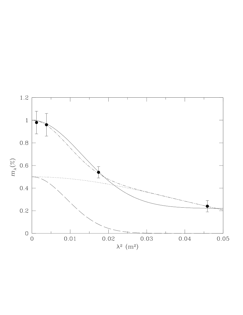
Figure 15: Simulation of a symmetric radio source at $45\degr$ from the plane of the sky with $LS=8$ kpc and $z=0.6$. The two Gaussians with $m_{0}=0.5$ (dashed and dotted lines) represent the depolarisation of the far and near lobes (respectively strongly and weakly depolarised) as a function of $\lambda^{2}$. The dash-dotted line is the sum of the two contributions. The “experimental” data points are values read from the model curve at the observed wavelengths of the present experiment. The continuous line is the fit to the four data points using Eq. 2 with $f_{c}=0.78$, i.e. assuming a partial source coverage.

We analyzed also the possible effects of intrinsic asymmetries in the source arm length. The two lobes suffer different depolarisations because the shorter arm, located closer to the centre, is inside the inner denser region of the medium (see Eq. 11). We made simulations, based on the arm-ratio distribution of  Rossetti  et al. (2006), for the 21 B3-VLA CSS sources for which a core is detected at 15 GHz. We found that, under the assumption of a spherically-symmetric Faraday medium, no significant effects are expected. The results might be different if the source asymmetries were caused by density asymmetries in the ISM  (Jeyakumar  et al. 2005), the denser ISM preventing one of the two lobes to grow like the other. In this case, the $\sigma_{\rm RM,sf}$ of the two lobes would differ not only because the shorter lobe is closer to the source centre (as before) but because, in addition, the ISM is denser on the short lobe side. We did not model this situation because it requires too many parameters that cannot be constrained easily. We used, instead, an experimental approach. For 13 of 21 sources observed at 15 GHz  (Rossetti  et al. 2006) that belong to the WSRT sub-sample, we plotted $f_{c}$ versus arm ratio. No significant relation has been found, suggesting that, if radio source asymmetries are due to ISM asymmetries, the latter are not very important in simulating a partial coverage effect.

In conclusion, we suggest that covering factors smaller than 0.8, are possibly justified by orientation effects.

6.9 Rotation Measures: A large-scale ordered magnetic field?

In the top panel of Fig. 16, we plot $\sigma_{\rm RM,obs}$ versus the observed, Galaxy-corrected, Rotation Measures, $RM_{\rm obs}$ for the 30 sources (21 with $z$) for which both data are available. We discuss possible selection effects in the plot. Sources for which $\sigma_{\rm RM,obs}\geq 70$ rad m^-2 and $f_{c}\geq 0.9$ should be strongly depolarised at 13 cm (Eq. 1), therefore their RMs are not measurable because the detectability at this wavelength is the condition we adopted to compute RM (Sect. 5.3). The 10 sources in the plot that have $\sigma_{\rm RM,obs}\geq 70$ rad m^-2, have $f_{c}\leq 0.9$.

Figure 16: Plot of $\sigma_{\rm RM}$ vs $RM$ in the observed (top panel) and in the source (bottom panel) frame. Open symbols in the top panel indicate Empty Fields. The tilted lines represent ($\sigma_{\rm RM,obs}/RM_{\rm obs}$) and ($\sigma_{\rm RM,sf}/RM_{\rm sf}$) = 10, 3, 1, 0.3, 0.1.

Because of band-width depolarisation, most sources with $RM_{\rm obs}\mathrel{>\kern-10.00002pt\lower 3.87495pt\hbox{$\sim$}}750$ rad  m^-2 would be depolarised at 13 cm and their RM would not be measurable. The vertical and horizontal lines show these limits. In the bottom panel of Fig. 16, we plot similar data, with the source frame parameters.

Both figures show that about half of the sources have $RM\geq\sigma_{\rm RM}$. This is unexpected for a model in which the magnetic field of the Faraday screen is random on small scales. Our Monte Carlo simulation (Sect. 5.2) shows that in these models the $E$ vector is expected to have, statistically, a small global rotation, with $|RM|\leq\sigma_{\rm RM}/\sqrt{N_{c}}$ (where $N_{c}$ is the ratio between source area and cell area) as long as $\sigma_{\rm RM}\lambda^{2}<2$ rad ($DP\mathrel{>\kern-10.00002pt\lower 3.87495pt\hbox{$\sim$}}5$%). If $N_{c}\gg 100$, the data points in Fig. 16 would be expected to cluster around or above the uppermost line, and, given the values we find for $\sigma_{\rm RM}$ (see Table 1), no large rotations of the polarisation angle with $\lambda^{2}$, the residual of the RM dispersion, are expected. In other words, with the possible exception of a minority of sources ($\leq 15\%$), the RMs are not the residuals of the random rotations that depolarise the radiation. They are likely generated on a larger scale by an ordered magnetic field component.

Figure 17: Plot of $RM_{\rm sf}$ vs (1+$z$)  (top panel) and of $RM_{\rm sf}$ vs LS (bottom panel). In both panels ($\vartriangle$) and ($\circ$) represent objects with $RM_{\rm sf}<$ and respectively $>\sigma_{\rm sf}$; filled symbols in the bottom panel represent objects with $z\geq 1$.

In Paper IV, we found a marginal correlation between $RM_{\rm sf}$ and $z$. In the top panel of Fig. 17, we plot $RM_{\rm sf}$ as a function of $(1+z)$. For $RM_{\rm sf}<100$ rad m^-2, the distribution in $z$ is uniform, while for $RM_{\rm sf}>100$ rad m^-2, 8 sources out of 10 have $z>1$. There is a hint of an upper bound that increases with $(1+z)$. The probability that the observed distribution is a random selection from a uniform redshift distribution is $\approx 7\%$. We further note that sources for which $RM_{\rm sf}\geq\sigma_{\rm RM,sf}$ (circles in Fig. 17, top panel) are distributed in a broad band such that $RM_{\rm sf}\propto(1+z)^{3}$. The probability that this is caused by a random selection from an uniform distribution is $\leq 1.5\%$. We have to examine if there are any biases which can affect the source distribution in the plot RM vs $(1+z)$. There are 10 sources for which we do not have a measured RM because they are depolarised at 13 cm. If these sources had an RM above the apparent upper bound in Fig. 17, (top panel), their RM would be high ($\geq 300$ rad m^-2) in the observer’s frame; we would expect therefore to see a rotation of the polarisation angle between 3.6 and 6 cm. At first sight there appear to be no candidates for these “missing RM” among the unpolarised sources at 13 cm. Although this statement has to be taken with some caution, we conclude that there is a real correlation between $RM_{\rm sf}$ and $(1+z)$, at least for sources for which $RM_{sf}\geq\sigma_{\rm RM,sf}$.

In the bottom panel of Fig. 17, we plot $RM_{\rm sf}$ versus LS. The distribution of data points is peculiar. There seems to be a “sequence” of sources, for $RM_{\rm sf}>100$ rad  m^-2, for which $RM_{\rm sf}\propto LS^{-2.2}$, which is a dependence on LS that is similar to that of $\sigma_{\rm RM,sf}$. This “sequence” (9 sources out of 21) is composed mainly of objects for which $RM_{\rm sf}>\sigma_{\rm RM,sf}$ (8 out of 9) and $z>1$ (7 out of 9). Of the remaining objects, $RM_{\rm sf}$ does not appear to show correlation with LS.

We conclude that for 50% of the CSS (mainly at high redshifts, $\langle z\rangle\approx 1.5$), a large-scale ordered magnetic field is present and produces the higher values of RMs. Its scale must be approximately 10–20 kpc to justify the correlation observed in the bottom panel of Fig. 17.

Applying a model similar to that for $\sigma_{\rm RM,sf}$ (Sect. 6.3) to the data of the “sequence” $RM_{\rm sf}$ versus LS, we find that the required ambient density and magnetic-field dependence on $r$, are similar to that for $\sigma_{\rm RM,sf}$ ($\beta+\mu\approx 1$), and $B_{||,0}\approx 40\,r_{c}^{-3}\,n_{0}^{-1}\approx 10\leavevmode\nobreak\ \mu$G, at the median $z\approx 1.9$ of the sources in the “sequence”. We observe that not all high-redshift objects lie on the $RM_{\rm sf}\propto LS^{-2.2}$ relation. A possible explanation is that in a large-scale magnetic-field, the orientation effects are important for RM. High-redshift sources that do not belong to the sequence, should have a line of sight that is at significant angles to the magnetic field.

If $B_{||,0}\,n_{0}\propto(1+z)^{4}$, as for $\sigma_{\rm RM,sf}$, at $z\leq 1$ the RM would drop to $\leq 150$ rad m^-2. Most of the low-redshift sources would fail to show the correlation of the high-redshift ones.

7 Summary and Conclusions

We have observed 65 radio sources from the B3-VLA CSS sample (Paper I) using the WSRT at 13 cm, to study the source polarisation properties. At the WSRT resolution, the radio sources are all unresolved, and we can therefore only discuss their global properties. The new 13-cm data, combined with earlier low-resolution VLA data at 3.6, 6, and 21 cm, have improved the determination of Rotation Measures ($RM$) and the Rotation Measure Dispersions ($\sigma_{\rm RM}$). This has allowed their properties to be defined more carefully as a function of both redshift and Linear Size, and the characteristics of the surrounding ISM to be modelled.

The main results of the paper are the following:

1)

Radio sources $\leq 5$ kpc are mostly unpolarised at 13 cm. This result is similar to results found at 20 cm (Cotton  et al. 2003) and at 3.6 and 6 cm (Paper IV), and the “critical size” that we find is intermediate between those found earlier.

2)

The 13 cm polarisation angles have led to a revision of the earlier $RM$s (Paper IV) for $\approx 30\%$ of the sources.

3)

The integrated fractional polarisation $m_{\lambda}$, as a function of wavelength shows in general a decrease between 3.6 and 13 cm, followed by a flattening between 13 and 20 cm. This is the major observational result of the present paper. At variance with the conclusions of  Paper IV, the  Burn (1966) and  Tribble (1991) models are not adequate to describe this behaviour. However, an empirical variant of the  Burn (1966) model, which introduces a “partial coverage” by the depolarising curtain, appears to reproduce the data well. The adopted formula allows the Rotation Measure Dispersion, $\sigma_{\rm RM}$, and the fraction, $f_{\rm c}$, of source covered by the depolarising curtain, to be determined.

4)

For a minority of sources, $m_{\lambda}$ shows an irregular, possibly oscillatory, behaviour with $\lambda$. We propose that these sources contain sub-components with different Rotation Measures that produce beats with $\lambda$ in the integrated fractional polarisation.

5)

$\sigma_{\rm RM}$ shows a clear dependence on redshift (up to $z\approx 1.8$), and on projected Linear Size.

6)

We have analysed these dependences using a model similar to that presented in  Paper IV, in which a depolarising Faraday curtain, with a King-like distribution of the magneto-ionic medium, is produced either by a smooth medium with an irregular magnetic field on small scales, or by a clumpy magnetised medium (NL region). The parameters derived in either case differ from those we obtained in  Paper IV, because of the use of the new 13 cm data and of the new model adopted for the depolarisation behaviour with $\lambda$. In both models the core radius of the curtain has to be $\leq 0.5$ kpc.

In the smooth medium model, the required central density, at $z=0$, is in the range of that found using X-ray observations in the centre of early-type galaxies. Beyond the core radius, it decreases according to $r^{-\eta}$, where $1.5\leq\eta\leq 2.0$. The central magnetic field, at $z=0$, is $\approx 150$ $\mu$G, and the magnetic field energy density is close to the thermal energy.

In the clumpy medium model, identified with the NLR, we assumed pressure equilibrum between the clouds and the diffuse medium in which they are embedded. The required magnetic field, inside the clouds at $z=0$, is $\approx 6\leavevmode\nobreak\ \mu$G, and the magnetic energy is a negligible ($\approx 10^{-4}$) fraction of the thermal energy. Beyond the core radius, the density of the smooth medium, which confines the clouds, should decline as $r^{-\eta}$, with $1.2\leq\eta\leq 1.6$. The product $B_{\rm NL,0}\times n_{\rm NL,0}$ is a strong function ($\propto(1+z)^{4}$) of redshift up to $z\approx 1.8$.

The $NL\leavevmode\nobreak\ model$ requires more parameters than the smooth medium model, and these parameters need tuning to avoid the “NL covering problem” discussed in Sect. 6.6. For these reasons, we favour the smooth medium model.

7)

The ISM density profiles required by the depolarisation models are consistent with the expectations of the evolutionary models of young radio sources.

8)

The partial coverage, that we introduced to describe the long wavelength behaviour of $m_{\lambda}$ vs $\lambda^{2}$, is probably due to orientations effects of the source with respect to the line of sight. For sources that are almost orthogonal to the line of sight, the two lobes are depolarised similarly by a spherically-symmetric medium, and $m_{\lambda}$ is fitted by the Burn model. However, when the source is at large angles with respect to the line of sight, the far lobe is more depolarised causing the rapid decrease of $m_{\lambda}$ at short wavelengths, while the nearby one is less depolarised giving rise to a lower decrement of $m_{\lambda}$ with wavelength. The total fractional polarisation $m_{\lambda}$ then appears to be almost constant at long wavelengths.

9)

The total source-frame Rotation Measures are generally too large to be the residual of random rotations across the source due to a totally irregular magnetic field, and require a large-scale ordered magnetic-field component. The Rotation Measures show hints of a correlation with both redshift and Linear Size in a way similar to the Rotation Measure dispersions. If these correlations are real, the ordered magnetic-field component would have parameters similar to those of the random field component.

Appendix A Polarisation Data

Table 1: Polarisation Data

Name	$S_{13}$	$m_{13}$	$\chi_{13}$	$RM_{\rm obs}$	$RM_{\rm sf}$	$\sigma_{\rm RM,obs}$	$\sigma_{\rm RM,sf}$	$m_{0}$	$f_{c}$	z	LS	Notes
(1)	(2)	(3)	(4)	(5)	(6)	(7)	(8)	(9)	(10)	(11)	(12)	(13)
0034+444	0.42	1.40$\pm$0.11	–33	–85	–72	41	589	3.1	0.9	2.79	11.9	P1, N
0039+373	0.60	0.10$\pm$0.10				243	982	1.0	0.85	1.01	0.5	P5
0039+398	0.48	0.34$\pm$0.11	42								16	P6
0039+412	0.25	2.81$\pm$0.12	–2	–100		22		5.2	0.64		8.5	P1, N, m
0041+425	0.30	0.28$\pm$0.13	(–24)			$>$368		3.0	0.93		4.1	P4
0049+379	0.46	0.27$\pm$0.11	(17)			254	1852	9.0	0.98	1.7	6.1	P3
0110+401	0.42	3.54$\pm$0.11	54	–65	–92	$\sim 8$	$\sim 49$	5.4	[1]	1.48	16.7	P1, N, m
0120+405	0.38	1.41$\pm$0.11	–102	–340	–880	140	474	5.5	0.75	0.84	10.1	P1, N
0123+402	0.16	1.32$\pm$0.15	–48	–136 a		$\leq$50		4.5	$\geq$0.95		5.2	P2
0128+394	0.20	0.55$\pm$0.14	–87	–150	–473	$\sim 10$	$\sim 68$	0.8	[1]	1.6	11.5	P5, N, m
0137+401	0.19	1.53$\pm$0.14	–30	–88 a	–55	$\leq$21	144	1.7	$\geq 0.4$	1.62	17.6	P1, N
0144+432	0.23	1.05$\pm$0.12	–40	–54	$+$132	105	536	3.5	0.66	1.26	17.2	P1, N
0147+400	0.51	0.01$\pm$0.10									0.4	P6
0213+412	0.39	0.63$\pm$0.11	10	–67 a	$+$30	63	146	3.1	0.89	0.52	7.3	P1
0222+422	0.16	0.39$\pm$0.14	(60)			195	3949	4.0	0.9	3.5	11.9	P3
0228+409A	0.24	1.60$\pm$0.12	38	–159		246		4.0	0.65		16.2	P1
0254+406	0.33	1.53$\pm$0.12	3	–27 a	$+$262	$\leq$20	$\leq$99	1.7	$\geq$0.25	1.22	18.9	P1
0255+460	0.45	0.10$\pm$0.11								1.21	3.2	NP
0701+392	0.35	0.15$\pm$0.12				102	512	1.0	0.8	1.24	7.8	P3
0722+393A	0.64	0.10$\pm$0.10									1.0	NP
0744+464	0.32	0.50$\pm$0.11	–3	–277 a	–4417	229	3537	5.5	0.9	2.93	5.1	P1, N
0748+413B	0.13	1.40$\pm$0.13	13	$+$29		201		18	0.94		1.8	P1
0754+396	0.33	8.32$\pm$0.13	–97	$+$5 a	–39	63	613	11.6	0.32	2.12	8.9	P1
0800+472	0.60	0.33$\pm$0.10	–54	–19	–64	148	337	2.4	0.83	0.51	3.7	P1
0805+406	0.37	5.75$\pm$0.12	2	$+$22 a		30		6.5	0.3		10.7	P1
0809+404	0.75	0.15$\pm$0.10				216	519	4.5	0.97	0.55	4.5	P3
0810+460B	0.66	0.11$\pm$0.10				$>$270	$>$478	2.0	0.94	0.33	3.0	P4
0814+441	0.17	1.93$\pm$0.12	–64	$+$352							17.0	P5, N
0822+394	0.77	0.02$\pm$0.10								1.18	0.2	NP
0840+424A	1.03	0.06$\pm$0.10									0.3	P6
0902+416	0.35	1.90$\pm$0.11	–65								1.4	P5, N
0930+389	0.17	2.79$\pm$0.12	–45	$+$46	$+$428	$\leq$24	$\leq$277	2.8	$\geq 0.8$	2.4	14.4	P1, N
0951+422	0.29	0.44$\pm$0.11	–3	$+7$	–15	206	1592	4.5	0.88	1.78	8.3	P1
0955+390	0.31	6.27$\pm$0.13	15	$+$15 a		$\leq$13		6.6	$\geq 0.6$		19.2	P1
1007+422	0.29	0.13$\pm$0.13				400		6.5	$\geq$0.95		0.55	P5
1025+390B	0.49	2.98$\pm$0.11	–101	–20	–54					0.36	9.7	P2, N, m
1027+392	0.28	0.26$\pm$0.11	(91)								6.9	P5, N
1039+424	0.17	6.90$\pm$0.15	–57	$+$12 a		$\leq$13		7.3	$\geq 0.8$		6.5	P1
1044+404A	0.25	0.35$\pm$0.11	14	$+$376	(9546)	155	($+$4032)	8.5	0.95	4.1	3.2	P2, N
1055+404A	0.25	5.69$\pm$0.12	0	$+$8.9 a		$\leq$13		5.9	$\geq 0.6$		12.1	P1
1128+455	1.35	0.00$\pm$0.10								0.40	2.9	NP
1136+420	0.32	0.20$\pm$0.11				$>$324	$>$1085	2.4	0.9	0.83	4.3	P4
1201+394	0.32	2.29$\pm$0.11	26	$+$38	$+$61	$\leq$24	$\leq$51	3.0	$\geq 0.90$	0.45	7.2	P1, N, m
1204+401	0.15	0.31$\pm$0.15	(–1)			68	641	5.2	$\geq$0.95	2.07	6.7	P3
1216+402	0.23	2.03$\pm$0.12	64	–190	–616	$\leq$10	$\leq 30$	4.0	[1]	0.76	15.5	P1, N, m
1220+408B	0.28	1.47$\pm$0.11	–100	$+$28 a		61		6.9	0.95		17.6	P1
1225+442	0.24	0.09$\pm$0.12								0.22	0.9	P6
1233+418	0.49	1.15$\pm$0.11	–52	–45	-84	50	78	4.3	$\geq$0.9	0.25	5.3	P2, N, m
1242+410	1.04	0.04$\pm$0.10								0.81	0.3	NP
1340+439	0.32	0.23$\pm$0.11	(–21)								0.3	P6, N
1343+386	0.66	0.38$\pm$0.11	–15	–379	–3129	115	928	3.8	0.86	1.84	0.5	P1, N, m
1350+432	0.09	3.18$\pm$0.16	–86	$+$230	$+$2193	150	1490	10.0	0.55	2.15	6.5	P1, N, m
1432+428B	0.66	0.15$\pm$0.10									0.2	P6
1441+409	0.67	0.10$\pm$0.10				$>$280		1.4	$\geq$0.9		0.4	P4
1449+421	0.43	0.12$\pm$0.10									0.3	NP
1458+433	0.29	2.70$\pm$0.11	12	–5 a	–52	$\leq$15	$\leq$55	2.7	$\geq 0.2$	0.93	6.9	P1, N
2301+443	0.69	0.03$\pm$0.10								1.7	2.1	P6
2302+402	0.83	0.10$\pm$0.10									2.6	P6, N
2304+377	1.07	0.19$\pm$0.10				182	357	3.2	0.96	0.4	0.3	P5
2311+469	1.38	4.22$\pm$0.11	–70	–8	$+$77	41	126	5.5	0.36	0.75	9.6	P1, N
2322+403	0.22	0.03$\pm$0.12				207		6.5	0.98		14.0	P3
2330+402	0.60	0.06$\pm$0.10									0.3	P6
2348+450	0.50	0.04$\pm$0.11				$>$290	1137	2.5	0.95	0.98	1.3	P4
2349+410	0.28	0.24$\pm$0.11	(76)							2.05	4.7	P5, N
2358+406	0.99	0.02$\pm$0.11									0.3	NP

- Columns 1, 2 and 3: Source Name, 13 cm flux density (Jy), fractional polarisation and error (%);

- Column 4: 13 cm Electric vector p.a. (degree) for sources with $m_{13}\geq 3\sigma_{m}$; values in parenthesis are for sources with $2\sigma_{m}\leq m_{13}\leq 3\sigma_{m}$. Errors, computed as in Sect. 3.1, are $\leq 9\degr$ for $m_{13}\geq 3\sigma_{m}$

- Columns 5 and 6: Observed and source frame Rotation Measure (rad m^-2). Formal errors of $RM_{\rm obs}$ are $\leq 10$ rad m^-2. An “a” near $RM_{\rm obs}$ means a good $\lambda^{2}$-linear fit (see Sect. 5.3).

- Columns 7 and 8: Observed and source frame $\sigma_{\rm RM}$ (rad m^-2); formal errors are typically $\leq 20$%

- Columns 9 and 10: Intrinsic Fractional polarisation (%) and Covering factor

- Columns 11, 12 and 13: Redshift (photometric one decimal digit only), Largest (projected) Linear Size (kpc), Notes

P1: the source is detected at $\geq 3\sigma_{\rm P}$ at all four wavelengths; P2: the source is detected at $\geq 3\sigma_{\rm P}$ at 3.6, 6, and 13 cm; P3: the source is detected at $\geq 3\sigma_{\rm P}$ at 3.6 and 6  cm; P4: the source is detected at $\geq 3\sigma_{\rm P}$ at 3.6  cm only; P5: the source is detected at $\geq 3\sigma_{\rm P}$ at two or three non contiguous wavelengths; P6: the source is detected at $\geq 3\sigma_{\rm P}$ at 21  cm only; NP: the source is undetected ($\leq 3\sigma_{\rm P}$) at all frequencies. N: see notes in Sect. A.1. m: data from the “two polarised component model” (see Notes and Appendix B).

A.1 Notes to individual sources

0034+444: See Fig. 8 and Sect. 5.3. The $\chi_{3.6}$ is discrepant from the $\chi(\lambda^{2})$ behaviour at the other frequencies, causing a poor overall fit. We have not been able to improve the fit using the “two polarised component model” of  B.

0039+412: The $RM_{\rm obs}$ obtained by a $\lambda^{2}$-linear fit, using also the individual IFs of the 13 cm band, does not properly account for $\chi_{21}$. We have used the “two polarised component model”, constrained by the polarisation structure seen by the VLA at 3.6 and 6  cm, which introduces a small modulation in the polarisation angles over the $\lambda^{2}$ behaviour which better fits all the data. The $RM_{\rm obs}$ in Table 1 is from this model.

0110+401: The source shows a deep minimum in fractional polarisation at $\approx 11$ cm (data from the Effelsberg telescope, see Klein  et al. (2003)). A $\lambda^{2}$-linear fit, using also the individual IFs of the 13 cm band, does not account for $\chi_{21}$. We have used the “two polarised component model” which fits very well both behaviours of $m_{\lambda}$ and $\chi(\lambda)$ vs $\lambda^{2}$ (see Fig. 6). The $RM_{\rm obs}$ and $\sigma_{\rm RM,obs}$ in Table 1 are from this model.

0120+405: An alternative value of $RM_{\rm obs}$ is $\approx-154$ rad  m^-2. The adopted $RM_{\rm obs}$ justifies the lack of polarisation at 21  cm as a bandwidth depolarisation effect. Both the reported $RM_{\rm obs}$ and the alternative one are in bad agreement with $RM_{13}$.

0128+394: This source shows a possible oscillatory behaviour of $m$ vs $\lambda^{2}$. We have used the “two polarised component model”, constrained by the polarisation structure seen by the VLA at 3.6 and 6 cm, which fits both $m$ and $\chi$ vs $\lambda^{2}$. The $RM_{\rm obs}$ and $\sigma_{\rm RM,obs}$ in Table 1 are from this model.

0137+401: The angle $\chi_{3.6}$ is in poor agreement with a $\lambda^{2}$-linear fit.

0144+432: The fitted $RM_{\rm obs}$ has a poor chi-square, mainly due to $\chi_{21}$. No acceptable two component model has been obtained to improve the fit.

0744+464: According to our $RM_{\rm obs}$ the fractional polarisation at 21 cm is depressed by a large factor because of bandwidth depolarisation.

0814+441: The source is undetected at 6 cm and well detected at the other three wavelengths, suggesting a possible oscillatory behaviour of $m$ vs $\lambda^{2}$. The two polarised component model quite fits the data except $\chi_{21}$ well. The fitted $RM_{\rm obs}$, which is very large, would imply virtually no polarisation at 21  cm because of bandwidth depolarisation, contrary to what is observed. However, the model shows strong modulations of $RM_{\rm obs}$, and at 21 cm the “local $RM_{\rm obs}$” is lower than the average, implying only a reduction of $m_{21}$ of a factor $\approx 2$, in agreement with the data.

0902+416: This is another source with a possible $m_{\lambda}$ oscillatory behaviour, being well detected at 3.6 and 13  cm but not at the other two wavelengths. We have modelled it with the two polarised component model; however, because of the small amount of data and lack of information on polarisation sub-structure, we consider the results too uncertain. No polarisation parameters are reported in Table 1.

0930+389: The $RM_{\rm obs}$ quoted in Table  1 is strongly constrained by $RM_{13}$. The angle $\chi_{3.6}$ is in bad agreement with the overall fit and causes a poor chi-square.

1025+390B: No data is available at 21 cm. The fractional polarisation $m_{3.6}$ is a factor $\approx 2$ lower than at 6 and 13 cm. It may be another case of oscillatory behaviour of $m_{\lambda}$. We have modelled the source with a two polarised component model, but, due to the limited amount of data, only $RM_{\rm obs}$ is given in Table 1.

1027+393: The source is strongly polarised at 6 and 21 cm but not at the other wavelengths. Therefore it is another case of oscillatory behaviour of $m_{\lambda}$. Although the two polarised component model fits both $m_{\lambda}$ and $\chi(\lambda)$, because of the limited amount of data the results are not properly constrained.

1044+404A: The very large $RM_{\rm obs}$ is likely the cause of the lack of polarisation at 21 cm because of bandwidth depolarisation.

1201+394: An improved fit of $\chi(\lambda)$ vs $\lambda^{2}$ is obtained by the “two polarised component model” which introduces a small modulation of the $\chi(\lambda)$ behaviour. Also the fit of the amplitudes is improved. The data in Table 1 are from this model.

1216+402: A possible oscillatory behaviour of $m_{\lambda}$ is well described by the “two polarised component model” which well fits $m_{\lambda}$ and $\chi(\lambda)$, except for $\chi_{21}$. $RM_{13}$ is somewhat lower than the adopted $RM_{\rm obs}$, but the model justifies it as a result of modulation of $\chi(\lambda)$ because of the beat between the two components. Data in Table 1 are from this model.

1233+418: The “two polarised component model”, based also on the polarisation substructure seen by the VLA at 3.6 and 21 cm, gives an improved fit to both $m_{\lambda}$ and $\chi(\lambda)$. The parameters in Table 1 are from this model.

1340+439: This source is well detected at 21 cm and possibly detected at $\geq 2\sigma_{\rm P}$ at 3.6 cm. It may be another example of the oscillatory behaviour of $m_{\lambda}$, which is easily fitted by the “two polarised component model”. However, because of to the poorness of the data we do not report any polarisation parameter.

1343+386: The angle $\chi_{3.6}$ is very discrepant with respect to the overall fit. Orienti  et al. (2004) showed that the polarisation is from the bright southern hot spot, and has substructures, with $RM_{\rm obs}$ differences $\approx 100$ rad  m^-2. We have applied the “two polarised component model” and obtained a much better fit for $m_{\lambda}$ and $\chi(\lambda)$, except for $\chi_{3.6}$ which we consider an outlier. The data in Table 1 are from this model.

1350+432: At a first sight there is a large discrepancy between $RM_{13}$ and the global $RM_{\rm obs}$. However, the “two polarised component model” properly fits the data, and justifies the low value of $RM_{13}$ as a result of modulation because of the beating of the two components. Data in Table 1 are from this model.

1458+433: $m_{3.6}=1.8\%$ is low compared to $m_{6}=2.6$%, $m_{13}=2.7$% and $m_{21}=2.4$%. We have no obvious explanation for this behaviour and have fitted $\sigma_{\rm RM,obs}$ with the exclusion of $m_{3.6}$.

2302+402: This source is detected at 21 cm only with a S/N = 17. The fractional polarisation is much larger than the upper limits at the other wavelengths.

2311+469: the angle $\chi_{3.6}$ is quite discrepant from the global $\chi(\lambda)$ fit.

2349+410: Undetected in polarisation at 6 and 13 cm. Another possible case of oscillatory behaviour of $m_{\lambda}$, which can be fitted by the “two polarised component model”. However, because of the poorness of the data we do not report any polarisation parameter.

Appendix B The two polarised component model

The polarisation status of a source can be represented by a vector of amplitude $S_{P}$ and position angle $2\chi$, defined in Sect. 3.2. When two sub-structures are present, different RMs in the two components may cause a differential rotation of the two polarisation vectors as a function of $\lambda^{2}$. The result is that the total source polarisation and $E$ vector position angle, under vectorial addition of the two component polarisation vectors, may present signs of interference. This produces, for instance, minima in $S_{P}(\lambda^{2})$ when the two polarisation vectors happen to be opposite.

We have applied this two polarised component model to a number of sources having one of the following characteristics:

i)

discrepancies between the $m_{\lambda}$ and the fitted model (Eq. 2), mostly possible oscillations of $m_{\lambda}$ vs $\lambda^{2}$, which could be indications of a beat between polarised subcomponents with different RM;

ii)

poor fit of the polarisation angles with the $\lambda^{2}$-linear law, again a possible indication of modulation which are due to polarised subcomponents with different RM. These sources should also exhibit beats, but there is only a marginal evidence for them. However, the oscillations might have been lost because of the limited $\lambda^{2}$ sampling or might have strongly been damped by depolarisation.

The parameters involved in the model are: the intrinsic fractional polarisation $m_{0}$, intrinsic position angle $\chi_{0}$ and RM of each component, and a common $\sigma_{\rm RM}$ and $f_{c}$ which accounts for the depolarisation. The available data are the $m_{\lambda}$ and $\chi(\lambda)$, (typically $2\times 4$ data), and $RM_{13}$ (Sect. 3.2.4) when available, so that we mostly have a comparable number of parameters and data points. It makes no sense to use more than two components in the model because the number of parameters would exceed the number of data.

In order to constrain the model as much as possible we used as starting parameters, when available, the data of the two more polarised components from the high resolution VLA data (Paper IV): i) $m_{3.6}$, ii) $RM^{3.6}_{6}$, iii) $\chi_{3.6}$ corrected to zero wavelength for $RM^{3.6}_{6}$. It has to be realized that $RM^{3.6}_{6}$ has an uncertainty $\geq 50$ rad  m^-2. Furthermore it is also possible that the beat is due to subcomponents unresolved even at our best VLA resolution, so that the input data would not be the relevant ones.

Sources of group i) are mostly fitted by the model, ranging from good and well constrained cases (see e.g. B3 0110+401) to less secure cases (e.g. B3 1340+439 and B3 2349+410 which are detected at two wavelengths only). The success is due to the fact that the fluctuations in $m_{\lambda}$ help in constraining some of the parameters, such as the difference between the two $RM$s and the intrinsic fractional polarisation $m_{0}$. For instance, undetected points are taken as deep minima in $m$. The level of success is definitely lower ($\leq 30$%) in the second group.

The results of the model have to be taken with caution because of the limited number of data points. When reasonably secure, we give the average RM, the common $\sigma_{\rm RM,obs}$ and $f_{c}$ and the intrinsic fractional polarisation $m_{0}$ (vectorial sum of $m(\lambda=0)$ of the two components).

Comments on individual fits are contained in the notes to individual sources (A.1).