Finite-frequency current (shot) noise in coherent resonant tunneling through a coupled-quantum-dot interferometer

Abstract

We examine the shot noise spectrum properties of coherent resonant tunneling in coupled quantum dots in both series and parallel arrangements by means of quantum rate equations and MacDonald’s formula. Our results show that, for a series-CQD with a relatively high dot-dot hopping $\Omega$, $\Omega/\Gamma\gtrsim 1$ ($\Gamma$ denotes the dot-lead tunnel-coupling strength), the noise spectrum exhibits a dip at the Rabi frequency, $2\Omega$, in the case of noninteracting electrons, but the dip is supplanted by a peak in the case of strong Coulomb repulsion; furthermore, it becomes a dip again for a completely symmetric parallel-CQD by tuning enclosed magnetic-flux.

I Introduction

The study of current noise through a quantum dot (QD) has recently become an emerging topic of interest in mesoscopic physics, because measurements of shot noise can yield more information about the microscopic mechanisms of transport than can conductance measurements alone.Blanter ; Beenakker In particular, finite-frequency noise provides direct access to the intrinsic dynamics of a mesoscopic system. For example, it has been reported that coherent intrinsic Rabi oscillations in coupled QDs (CQD) causes a dip at the Rabi frequency in the noise spectrum.Sun ; Aguado ; Djuric ; Djuric1 On the contrary, a peak at the Zeeman frequency in the noise spectrum has been addressed for the coherent magnetotransport through an interacting QD with Zeeman-splitting levels.Fedichkin Later, the authors have analyzed further the role of Coulomb interaction in the magnetotransport through a QD and pointed out that the noise spectrum indeed exhibits a peak at the Zeeman frequency in the regime of Coulomb blockade, but it becomes a dip for noninteracting electrons.Gurvitz3 So it is natural to ask what will happen in the noise spectrum of a CQD if the interdot Coulomb interaction is taken into account. This constitutes the first purpose of the present paper.

On the other hand, coherent tunneling through a CQD in a parallel arrangement between two electrodes is quite interesting and has attracted numerous investigations because both interdot coherence and also quantum interference between two distinct magnetic-flux pathways play an important role in determining the transport properties of this system.Holleitner1 ; Holleitner2 ; ChenJ ; Shahbazyan ; Loss ; Konig ; Kubala ; Ladron ; Dong1 The interference pattern can be changed from destructive to constructive by tuning the magnetic-flux piercing the enclosed two pathways. Even though it has been reported that the interference effect produces a peak or a dip in the noise spectrum of a QD with two energy levels, depending on the relative phase of the two levels carrying the current,GurvitzIEEE yet it is not quite clear about the combination of the interdot Coulomb repulsion and interference effect, which is the second purpose of our studies.

In this paper, we analyze finite-frequency shot noise of first-order coherent tunneling through a CQD in both series and parallel configurations using quantum rate equations (QREs) and MacDonald’s formula. In Sec. II, we introduce the model Hamiltonian of the system under investigation. In the following two sections, we consider the two cases of noninteracting electrons and interacting electrons respectively. In these sections, we discuss the respective number-resolved QREs for describing first-order resonant tunneling at extremely high bias-voltage, which can be obtained from our previous derivation.Dong1 ; Dong4 Then we apply MacDonald’s scheme to calculate the tunneling current and its noise spectrum.Gurvitz3 ; MacDonald In particular, we derive explicit analytical expressions for the noise spectrum and charge fluctuation spectrum of a series-CQD and a completely symmetric parallel-CQD. In Sec. V, we present numerical calculations and point out how strong Coulomb repulsion and quantum interference influence the noise spectrum. We find that the noise spectrum exhibits a dip at the Rabi frequency for a noninteracting series-CQD with large dot-dot hopping strength, but the dip is supplanted by a peak in the case of strong Coulomb repulsion. As the coupling strength of the additional path branch is increased, the Coulomb interaction-induced peak in the noise spectrum gradually becomes a Fano-type peak, and finally emerges as a dip in the case of nonzero enclosed magnetic-flux. Sec. VI summaries our conclusions.

II Model Hamiltonian

The Hamiltonian of the parallel-CQD interferometer connected to two normal leads is written as

$$H=H_{L}+H_{R}+H_{D}+H_{T},$$ (1)

with

$$H_{\eta} = \sum_{{\bf k}}\varepsilon_{\eta{\bf k}}a_{\eta{\bf k}}^{\dagger}a_{\eta{\bf k}}^{\phantom{\dagger}},$$ (2)

$$H_{D} = \sum_{j=1,2}\varepsilon_{j}c_{j}^{\dagger}c_{j}^{\phantom{\dagger}}+Uc_{1}^{\dagger}c_{1}^{\phantom{\dagger}}c_{2}^{\dagger}c_{2}^{\phantom{\dagger}}+\Omega(c_{1}^{\dagger}c_{2}^{\phantom{\dagger}}+c_{2}^{\dagger}c_{1}^{\phantom{\dagger}}),$$ (3)

$$H_{T} = \sum_{{\bf k}}[(V_{L1}e^{i\varphi/4}a_{L{\bf k}}^{\dagger}+V_{R1}e^{-i\varphi/4}a_{R{\bf k}}^{\dagger})c_{1}$$ (5)

$$+(V_{L2}e^{-i\varphi/4}a_{L{\bf k}}^{\dagger}+V_{R2}e^{i\varphi/4}a_{R{\bf k}}^{\dagger})c_{2}+{\rm{H.c.}}],$$

where $a_{\eta{\bf k}}^{\dagger}$ ($a_{\eta{\bf k}}$) is the creation (annihilation) operator of an electron with momentum ${\bf k}$, and energy $\varepsilon_{\eta{\bf k}}$ in lead $\eta$($=L,R$), and $c_{j}^{\dagger}$ ($c_{j}$) is the creation (annihilation) operator for a spinless electron with energy $\varepsilon_{j}$ in the $j$th QD ($j=1,2$). $\varepsilon_{1(2)}=\varepsilon_{d}\pm\delta$, with $\delta$ being the bare mismatch between the two bare levels. $U$ represents the interdot Coulomb interaction, and $\Omega$ denotes hopping strength between the two QDs. $V_{\eta j}$ represents the tunneling matrix element between lead $\eta$ and dot $j$, and is assumed to be real and independent of energy. In this paper, we assume $V_{L1}=V_{R2}$ and $V_{L2}=V_{R1}$. The factor $e^{\pm i\varphi/4}$ is the accumulated Peierls phase due to the magnetic-flux $\Phi$ ($\varphi\equiv 2\pi\Phi/\Phi_{0}$, $\Phi_{0}\equiv hc/e$ is the magnetic-flux quantum) which penetrates the area enclosed by the two tunneling pathways of the Aharonov-Bohm (AB) interferometer. Such a QD AB interferometer has been realized in recent experiments.Holleitner1 ; Holleitner2 ; ChenJ Furthermore, we assume the two electrodes to be Markovian stationary reservoirs with a flat density of states $\varrho$.

In this coupled-QD (CQD) system, there are a total of four possible states for the present system: (1) the whole system is empty, $|0\rangle_{1}|0\rangle_{2}$, and its energy is zero; (2) the first QD is singly occupied by an electron, $|1\rangle_{1}|0\rangle_{2}$, and its energy is $\varepsilon_{1}$; (3) the second QD is singly occupied, $|0\rangle_{1}|1\rangle_{2}$, and its energy is $\varepsilon_{2}$; and (4) both QDs are occupied, $|1\rangle_{1}|1\rangle_{2}$, and its energy is $\varepsilon_{1}+\varepsilon_{2}+U$. Of course, if the interdot Coulomb repulsion is assumed to be infinite, the double-occupation is prohibited. Therefore, as far as the four possible single electronic states are considered as the basis, the density-matrix elements are expressed as $\hat{\rho}_{00}=|0\rangle_{1}|0\rangle_{2}{}_{2}\langle 0|{}_{1}\langle 0|$, $\hat{\rho}_{11}=|1\rangle_{1}|0\rangle_{2}{}_{2}\langle 0|{}_{1}\langle 1|$, $\hat{\rho}_{22}=|0\rangle_{1}|1\rangle_{2}{}_{2}\langle 1|{}_{1}\langle 0|$, $\hat{\rho}_{dd}=|1\rangle_{1}|1\rangle_{2}{}_{2}\langle 1|{}_{1}\langle 1|$, and $\hat{\rho}_{12}=|1\rangle_{1}|0\rangle_{2}{}_{2}\langle 1|{}_{1}\langle 0|$. The statistical expectation values of the diagonal elements of the density-matrix, $\rho_{00}=\langle\hat{\rho}_{00}\rangle$, $\rho_{jj}=\langle\hat{\rho}_{jj}\rangle$ ($j=1,2$), and $\rho_{dd}=\langle\hat{\rho}_{dd}\rangle$ describe the occupation probabilities of the electronic levels for the system being empty, singly occupied in the $j$th QD by an electron, or doubly occupied in both QDs, respectively. The off-diagonal term $\rho_{12}=\langle\hat{\rho}_{12}\rangle$ describes the coherent superposition of two electronic single occupation states, $|1\rangle_{1}|0\rangle_{2}$ and $|0\rangle_{1}|1\rangle_{2}$.

In the limit of sufficiently large bias-voltage [$V\gg\Gamma,\Gamma^{\prime}$ (the tunnel-coupling strengths between dots and leads, which are defined below), and $\Omega$], electronic tunneling through this system in the first-order approximation can be described by recently derived QREs for the dynamic evolution of the reduced density matrix elements of the CQD, $\rho_{ab}(t)$ ($a,b=\{0,1,2,d\}$).Dong1 ; GurvitzIEEE ; Dong4 ; Stoof ; Gurvitz ; Gurvitz1 ; Dong In the following, we employ MacDonald’s formula, in conjunction with the number-resolved QREs, to evaluate the noise spectrum of coherent resonant tunneling in a CQD.

III CQD in the case of extremely large bias-voltage and no interdot Coulomb repulsion

First, we consider the absence of interdot Coulomb repulsion, $U=0$, in the case of extremely large bias-voltage and zero temperature. Throughout, we will use units with $\hbar=k_{B}=e=1$.

III.1 Number-resolved QREs

In the discussion of frequency-dependent current noise in the CQD interferometer, we employ MacDonald’s formula for shot noiseMacDonald based on the number-resolved version of the QREs, in accordance with the number of achieved tunneling events.Chen We introduce the number-resolved density matrices $\rho_{ab}^{(n)}(t)$ ($a,b=\{0,1,2,d\}$), representing the probability that the system is in the electronic state $|a\rangle$ ($a=b$), or in the quantum superposition state ($a\neq b$), at time $t$ together with $n$ electrons entering into the left lead due to tunneling events. Obviously, $\rho_{ab}(t)=\sum_{n}\rho_{ab}^{(n)}(t)$ and the associated number-resolved QREs in the case of extremely large bias-voltage and zero temperature are:

$$\dot{\rho}_{00}^{(n)} = \Gamma^{\prime}\rho_{11}^{(n-1)}+\Gamma\rho_{22}^{(n-1)}-(\Gamma+\Gamma^{\prime})\rho_{00}^{(n)}$$ (6b)

$$+\sqrt{\Gamma\Gamma^{\prime}}(e^{-i\varphi/2}\rho_{12}^{(n-1)}+e^{i\varphi/2}\rho_{21}^{(n-1)}),$$

$$\dot{\rho}_{11}^{(n)} = \Gamma\rho_{00}^{(n)}-2\Gamma^{\prime}\rho_{11}^{(n)}+\Gamma\rho_{dd}^{(n-1)}+i\Omega(\rho_{12}^{(n)}-\rho_{21}^{(n)})$$ (6d)

$$-\frac{1}{2}\sqrt{\Gamma\Gamma^{\prime}}(e^{-i\varphi/2}-e^{i\varphi/2})(\rho_{12}^{(n)}-\rho_{21}^{(n)}),$$

$$\dot{\rho}_{22}^{(n)} = \Gamma^{\prime}\rho_{00}^{(n)}-2\Gamma\rho_{22}^{(n)}+\Gamma^{\prime}\rho_{dd}^{(n-1)}-i\Omega(\rho_{12}^{(n)}-\rho_{21}^{(n)})$$ (6f)

$$-\frac{1}{2}\sqrt{\Gamma\Gamma^{\prime}}(e^{-i\varphi/2}-e^{i\varphi/2})(\rho_{12}^{(n)}-\rho_{21}^{(n)}),$$

$$\dot{\rho}_{dd}^{(n)} = \Gamma^{\prime}\rho_{11}^{(n)}+\Gamma\rho_{22}^{(n)}-(\Gamma+\Gamma^{\prime})\rho_{dd}^{(n)}$$ (6h)

$$-\sqrt{\Gamma\Gamma^{\prime}}e^{i\varphi/2}\rho_{12}^{(n)}-\sqrt{\Gamma\Gamma^{\prime}}e^{-i\varphi/2}\rho_{21}^{(n)},$$

$$\dot{\rho}_{12}^{(n)} = i\Omega(\rho_{11}^{(n)}-\rho_{22}^{(n)})-(\Gamma+\Gamma^{\prime})\rho_{12}^{(n)}$$ (6k)

$$+\sqrt{\Gamma\Gamma^{\prime}}e^{-i\varphi/2}\rho_{00}^{(n)}-\sqrt{\Gamma\Gamma^{\prime}}e^{i\varphi/2}\rho_{dd}^{(n-1)}$$

$$-\frac{1}{2}\sqrt{\Gamma\Gamma^{\prime}}(e^{i\varphi/2}-e^{-i\varphi/2})(\rho_{11}^{(n)}+\rho_{22}^{(n)}),$$

together with the normalization relation $\rho_{00}+\rho_{11}+\rho_{22}+\rho_{dd}=1$. The adjoint equation of Eq. (6k) gives the equation of motion for $\rho_{21}^{(n)}$. The constant parameters $\Gamma=2\pi\varrho_{L}|V_{L1(R2)}|^{2}$ and $\Gamma^{\prime}=2\pi\varrho_{L}|V_{L2(R1)}|^{2}$ represent the strengths of tunnel-couplings between dots and leads; $\sqrt{\Gamma\Gamma^{\prime}}$ describes the interference in tunneling events arising from different pathways. From these number-resolved QREs, we can readily deduce the usual QREs for the reduced density matrix elements, ${\bm{\rho}}(t)=(\rho_{00},\rho_{11},\rho_{22},\rho_{dd},\rho_{12},\rho_{21})^{T}$, as:

$$\dot{\bm{\rho}}(t)={\cal M}{\bm{\rho}}(t),$$ (7)

where ${\cal M}$ can be easily read from Eqs. (6b)-(6k) as:

$${\cal M}=\left(\begin{array}[]{cccccc}-(\Gamma+\Gamma^{\prime})&\Gamma^{\prime}&\Gamma&0&\sqrt{\Gamma\Gamma^{\prime}}e^{-i\varphi/2}&\sqrt{\Gamma\Gamma^{\prime}}e^{i\varphi/2}\\ \Gamma&-2\Gamma^{\prime}&0&\Gamma&-i\Omega-\frac{\sqrt{\Gamma\Gamma^{\prime}}}{2}e^{-i\varphi/2}&i\Omega-\frac{\sqrt{\Gamma\Gamma^{\prime}}}{2}e^{i\varphi/2}\\ \Gamma^{\prime}&0&-2\Gamma&\Gamma^{\prime}&i\Omega-\frac{\sqrt{\Gamma\Gamma^{\prime}}}{2}e^{-i\varphi/2}&-i\Omega-\frac{\sqrt{\Gamma\Gamma^{\prime}}}{2}e^{i\varphi/2}\\ 0&\Gamma^{\prime}&\Gamma&-(\Gamma+\Gamma^{\prime})&-\sqrt{\Gamma\Gamma^{\prime}}e^{i\varphi/2}&-\sqrt{\Gamma\Gamma^{\prime}}e^{-i\varphi/2}\\ \sqrt{\Gamma\Gamma^{\prime}}e^{-i\varphi/2}&i\Omega-i\sqrt{\Gamma\Gamma^{\prime}}\sin(\varphi/2)&-i\Omega-i\sqrt{\Gamma\Gamma^{\prime}}\sin(\varphi/2)&-\sqrt{\Gamma\Gamma^{\prime}}e^{i\varphi/2}&-\frac{1}{2}(\Gamma+\Gamma^{\prime})&0\\ \sqrt{\Gamma\Gamma^{\prime}}e^{i\varphi/2}&-i\Omega+i\sqrt{\Gamma\Gamma^{\prime}}\sin(\varphi/2)&i\Omega+i\sqrt{\Gamma\Gamma^{\prime}}\sin(\varphi/2)&-\sqrt{\Gamma\Gamma^{\prime}}e^{-i\varphi/2}&0&-\frac{1}{2}(\Gamma+\Gamma^{\prime})\end{array}\right),$$ (8)

The current flowing through the system can be evaluated as the time rate of change of electron number in the right lead

$$I_{R}(t)=\dot{N}_{R}(t)=\frac{d}{dt}\sum_{n}nP^{(n)}(t),$$ (9)

where

$$P^{(n)}(t)=\rho_{00}^{(n)}(t)+\rho_{11}^{(n)}(t)+\rho_{22}^{(n)}(t)+\rho_{dd}^{(n)}(t)$$ (10)

is the total probability of transferring $n$ electrons into the right lead by time $t$. From the number-resolved QREs, Eqs. (6b)–(6k), it is readily shown that $I_{R}(t)$ is given by:

$$I_{R}(t) = \Gamma^{\prime}\rho_{11}+\Gamma\rho_{22}+(\Gamma+\Gamma^{\prime})\rho_{dd}$$ (12)

$$+\sqrt{\Gamma\Gamma^{\prime}}(e^{-i\varphi/2}\rho_{12}+e^{i\varphi/2}\rho_{21}).$$

Substituting the stationary solution for ${\bm{\rho}}_{st}$ of Eq. (7) into Eq. (12), we can evaluate the stationary current $I$. In particular, we obtain analytical expressions for several magnetic-fluxes, $\varphi$: ($x=\Omega/\Gamma$ and $\gamma=\Gamma^{\prime}/\Gamma$)

$$I=\left\{\begin{array}[]{ccl}\frac{2(\gamma+1)(\gamma+x^{2})}{(\gamma+1)^{2}+4x^{2}}\Gamma,&&\text{$\varphi=0$ and $2\pi$}\\ \frac{2(\gamma+1)x^{2}}{(\gamma+1)^{2}+4x^{2}}\Gamma,&&\varphi=\pm\pi.\end{array}\right.$$ (13)

If $\Gamma^{\prime}=0$ ($\gamma=0$), the system reduces to a series-CQD, and, correspondingly, the stationary current becomes

$$I=\frac{2x^{2}}{1+4x^{2}}\Gamma.$$ (14)

On the other hand, for a completely symmetrical parallel-CQD, $\Gamma^{\prime}=\Gamma$ ($\gamma=1$), we have

$$I=\left\{\begin{array}[]{ccl}\Gamma,&&\text{$\varphi=0$ and $2\pi$}\\ \frac{x^{2}}{1+x^{2}}\Gamma,&&\varphi=\pm\pi.\end{array}\right.$$ (15)

III.2 MacDonald’s formula for shot noise spectrum

The frequency-dependent shot noise spectrum with respect to the right lead can be defined in terms of $P^{(n)}(t)$ using the standard technique based on MacDonald’s formula:MacDonald

$$S_{R}(\omega)=2\omega\int_{0}^{\infty}dt\sin(\omega t)\left[\frac{d}{dt}\sum_{n}n^{2}P^{(n)}(t)-2I^{2}t\right].$$ (16)

In this formulation, the long-time linear behavior of the first term inside the square brackets on the right hand side is canceled by the latter term, $2I^{2}t$. Then the noise spectrum can be evaluated in the form

$$S_{R}(\omega)=i\omega[{\cal P}(i\omega)-{\cal P}(-i\omega)],$$ (17)

with

$${\cal P}(s)=\int_{0}^{\infty}dt\,e^{-st}\frac{d}{dt}\sum_{n}n^{2}P^{(n)}(t).$$ (18)

Here, the stationary-current-related term of Eq. (16) gives no contribution.

To evaluate $S_{R}(\omega)$, we define an auxiliary function $G_{ab}(t)$ as

$$G_{ab}(t)=\sum_{n}n\rho_{ab}^{(n)}(t),$$ (19)

whose equations of motion can be readily deduced employing the number-resolved QREs, Eqs (6b)–(6k), in matrix form:

$$\dot{\bm{G}}(t)={\cal M}{\bm{G}}(t)+{\cal G}{\bm{\rho}}(t),$$ (20)

with ${\bm{G}}(t)=(G_{00},G_{11},G_{22},G_{dd},G_{12},G_{21})^{T}$ and

$${\cal G}=\left(\begin{array}[]{cccccc}0&\Gamma^{\prime}&\Gamma&0&\sqrt{\Gamma\Gamma^{\prime}}e^{-i\varphi/2}&\sqrt{\Gamma\Gamma^{\prime}}e^{i\varphi/2}\\ 0&0&0&\Gamma&0&0\\ 0&0&0&\Gamma^{\prime}&0&0\\ 0&0&0&0&0&0\\ 0&0&0&-\sqrt{\Gamma\Gamma^{\prime}}e^{i\varphi/2}&0&0\\ 0&0&0&-\sqrt{\Gamma\Gamma^{\prime}}e^{-i\varphi/2}&0&0\end{array}\right).$$ (21)

With the help of the number-resolved QREs Eqs. (6b)–(6k), we find

$${\cal P}(s) = \bigl{(}\Gamma^{\prime}[2G_{11}(s)+\rho_{11}(s)]+\Gamma[2G_{22}(s)+\rho_{22}(s)]$$ (25)

$$+(\Gamma+\Gamma^{\prime})[2G_{dd}(s)+\rho_{dd}(s)]$$

$$+\sqrt{\Gamma\Gamma^{\prime}}\left\{e^{-i\varphi/2}[2G_{12}(s)+\rho_{12}(s)]\right.$$

$$\left.+e^{i\varphi/2}[2G_{21}(s)+\rho_{21}(s)]\right\}\bigr{)},$$

where $G_{ab}(s)$ and $\rho_{ab}(s)$ are the Laplace transforms of $G_{ab}(t)$ and $\rho_{ab}(t)$, respectively:

$$G(\rho)_{ab}(s)=\int_{0}^{\infty}dt\,e^{-st}G(\rho)_{ab}(t).$$ (26)

Accordingly, we can readily evaluate ${\bm{\rho}}(s)$ by Laplace transforming its equation of motion, Eq. (7), with the initial condition, ${\bm{\rho}}(0)={\bm{\rho}}_{st}$:

$${\bm{\rho}}(s)=(s{\bm{I}}-{\cal M})^{-1}{\bm{\rho}}_{st}.$$ (27)

Thus, applying the Laplace transform to Eq. (20) yields

$${\bm{G}}(s)=(s{\bm{I}}-{\cal M})^{-1}{\cal G}{\bm{\rho}}(s).$$ (28)

Substituting the Laplace transform solutions for ${\bm{G}}(s)$ and ${\bm{\rho}}(s)$ into Eqs. (25) and (17), we can evaluate the noise spectrum. It should be noted that due to the inherent long-time stability of the physical system under consideration, all real parts of the nonzero poles of ${\bm{\rho}}(s)$ and ${\bm{G}}(s)$ are negative definite. Consequently, the divergent terms of the partial fraction expansions of ${\bm{\rho}}(s)$ and ${\bm{G}}(s)$ at $s\rightarrow 0$ entirely determine the long-time behavior of the auxiliary functions, i.e., the zero-frequency shot noise, Eq. (16) at $\omega=0$.Dong4

Furthermore, according to the Ramo-Shockley theorem,Ramo ; Shockley the average current $I_{c}$ is given by

$$I_{c}(t)=\alpha I_{L}(t)+\beta I_{R}(t).$$ (29)

Here the coefficients $\alpha$ and $\beta$, which satisfy $\alpha+\beta=1$, depend on the barrier geometry. For simplicity we take $\alpha=\beta=\frac{1}{2}$. Considering charge conservation, $I_{L}=I_{R}+\dot{Q}$, with

$$Q(t)=\sum_{n}[\rho_{11}^{(n)}(t)+\rho_{22}^{(n)}(t)+2\rho_{dd}^{(n)}(t)]$$ (30)

as the total charge in the CQD,Korotkov we have

$$I_{c}(t)I_{c}(0)=\alpha I_{L}(t)I_{L}(0)+\beta I_{R}(t)I_{R}(0)-\alpha\beta\dot{Q}(t)\dot{Q}(0).$$ (31)

Thus, the total noise spectrum is given by

$$S(\omega)=\alpha S_{L}(\omega)+\beta S_{R}(\omega)-\alpha\beta\omega^{2}S_{Q}(\omega),$$ (32)

where $S_{L}(\omega)$ is the noise spectrum with regard to the left lead and $S_{Q}(\omega)$ is the Fourier transform of the symmetrical charge correlation function. Generally, one can show that $S_{L}(\omega)=S_{R}(\omega)$ and calculate $S_{Q}(\omega)$ asGurvitz3

$$S_{Q}(\omega)=2[{\cal Q}(i\omega)+{\cal Q}(-i\omega)],$$ (33)

with

$${\cal Q}(s) = \int_{0}^{\infty}dt\,e^{-st}Q(t)$$ (34)

$$= \rho_{11}^{\prime}(s)+\rho_{22}^{\prime}(s)+2\rho_{dd}^{\prime}(s).$$ (35)

Likewise, we evaluate the Laplace transform solution for ${\bm{\rho}}^{\prime}(s)=(\rho_{00}^{\prime},\rho_{11}^{\prime},\rho_{22}^{\prime},\rho_{dd}^{\prime},\rho_{12}^{\prime},\rho_{21}^{\prime})^{T}$ with the associated initial condition, ${\bm{\rho}}^{\prime}(0)=(0,\rho_{11}^{st},\rho_{22}^{st},\rho_{dd}^{st},0,0)^{T}$, through

$${\bm{\rho}}^{\prime}(s)=(s{\bm{I}}-{\cal M})^{-1}{\bm{\rho}}^{\prime}(0).$$ (36)

Straightforwardly, we obtain analytical expressions for the frequency-dependent noise for several special cases. When $\Gamma^{\prime}=0$, i.e. for a series-CQD, we have (hereafter, we use $\omega$ to denote the normalized frequency $\omega/\Gamma$)

$$S_{R}(\omega) = S_{0}+S_{1}(\omega)+S_{2}(\omega),$$ (37a)

$$S_{0} = \frac{4x^{2}(8x^{4}-2x^{2}+1)}{(1+4x^{2})^{3}}\Gamma,$$ (37b)

$$S_{1}(\omega) = \frac{2x^{2}}{1+4x^{2}}\frac{\omega^{2}}{\omega^{2}+1}\Gamma,$$ (37c)

$$S_{2}(\omega) = -\frac{\omega^{2}[(1-12x^{2})\omega^{2}+80x^{4}-40x^{2}+1]}{[(\omega+2x)^{2}+1][(\omega-2x)^{2}+1]}$$ (37e)

$$\times\frac{2x^{2}}{(1+4x^{2})^{3}}\Gamma,$$

and

$$S_{Q}(\omega)=\frac{8x^{2}}{(1+4x^{2})(\omega^{2}+1)}\Gamma.$$ (37f)

It can be obtained from Eq. (37e) that $S(\omega)$ has a peak at $\omega=2x$ if $x<1$, but a dip otherwise [see Fig. 1(a) below]. If $\Gamma^{\prime}=\Gamma$ ($\gamma=1$), i.e. a CQD in a completely symmetrical parallel arrangement, we have

$$S_{R}(\omega) = S_{0}+S_{1}(\omega),$$ (38a)

$$S_{0} = \Gamma,$$ (38b)

$$S_{1}(\omega) = \frac{\omega^{2}}{\omega^{2}+16}\Gamma,$$ (38c)

$$S_{Q}(\omega) = \frac{4}{\omega^{2}+16}\Gamma,$$ (38d)

for $\varphi=0$; and for $\varphi=\pm\pi$ we obtain

$$S_{R}(\omega) = S_{0}+S_{1}(\omega),$$ (39a)

$$S_{0} = \frac{x^{2}(x^{4}-x^{2}+2)}{(1+x^{2})^{3}}\Gamma,$$ (39b)

$$S_{1}(\omega) = x^{4}\omega^{2}[(5+x^{2})\omega^{4}+(60-28x^{2}-8x^{4})\omega^{2}+16x^{6}$$ (39e)

$$+64x^{4}+16x^{2}+224]\Gamma(1+x^{2})^{-3}(\omega^{2}+4)^{-1}$$

$$\times\{[(\omega-2x)^{2}+4][(\omega+2x)^{2}+4]\}^{-1},$$

$$S_{Q}(\omega) = \frac{4x^{2}}{(1+x^{2})(\omega^{2}+4)}\Gamma.$$ (39f)

The frequency-dependent part of the noise is thus

$$S(\omega)-S_{0} = \frac{\omega^{2}[(3x^{2}-1)\omega^{2}-20x^{2}(x^{2}-2)-4]}{[(\omega-2x)^{2}+4][(\omega+2x)^{2}+4]}$$ (41)

$$\times\frac{x^{2}}{(1+x^{2})^{3}}\Gamma,$$

which indicates that the noise spectrum exhibits an unambiguous dip only when $x\gtrsim 2$ (this is different from the case of series-CQD revealed above).

IV Coulomb repulsion effect on finite-frequency shot noise

This section is concerned with the effects of strong Coulomb repulsion ($U=\infty$) on the noise spectrum in the case of an extremely large bias-voltage and zero temperature. In fact, the time-oscillatory current is no longer spatially translationally invariant at finite frequency due to a time dependent charge accumulation in the device. Coulomb interactions among electrons screen this accumulation and therefore can significantly influence the noise spectrum.Hanke ; Korotkov

In this case, the probability for a double-occupation state completely vanishes, $\rho_{dd}=0$, and the corresponding number-resolved QREs are:

$$\dot{\rho}_{11}^{(n)} = \Gamma\rho_{00}^{(n)}-\Gamma^{\prime}\rho_{11}^{(n)}+i\Omega(\rho_{12}^{(n)}-\rho_{21}^{(n)})$$ (42b)

$$-\frac{1}{2}\sqrt{\Gamma\Gamma^{\prime}}(e^{-i\varphi/2}\rho_{12}^{(n)}+e^{i\varphi/2}\rho_{21}^{(n)}),$$

$$\dot{\rho}_{22}^{(n)} = \Gamma^{\prime}\rho_{00}^{(n)}-\Gamma\rho_{22}^{(n)}-i\Omega(\rho_{12}^{(n)}-\rho_{21}^{(n)})$$ (42d)

$$-\frac{1}{2}\sqrt{\Gamma\Gamma^{\prime}}(e^{-i\varphi/2}\rho_{12}^{(n)}+e^{i\varphi/2}\rho_{21}^{(n)}),$$

$$\dot{\rho}_{12}^{(n)} = i\Omega(\rho_{11}^{(n)}-\rho_{22}^{(n)})-\frac{1}{2}(\Gamma+\Gamma^{\prime})\rho_{12}^{(n)}$$ (42f)

$$+\sqrt{\Gamma\Gamma^{\prime}}e^{-i\varphi/2}\rho_{00}^{(n)}-\frac{1}{2}\sqrt{\Gamma\Gamma^{\prime}}e^{i\varphi/2}(\rho_{11}^{(n)}+\rho_{22}^{(n)}),$$

together with the normalization relation $\rho_{00}+\rho_{11}+\rho_{22}=1$. The equation of motion for $\rho_{00}^{(n)}$ is the same as Eq. (6b).

Following the same procedures as indicated in the preceding section, we can evaluate the stationary current

$$I=\frac{4(\gamma+1)x^{2}}{(\gamma+1)^{2}+12x^{2}}\Gamma,$$ (43)

and shot noise spectrum for the case of strong Coulomb blockade. Straightforwardly, we again obtain analytical expressions for frequency-dependent noise in several special cases. For a series-CQD, we have

$$S_{R}(\omega) = S_{0}+S_{1}(\omega),$$ (44a)

$$S_{0} = \frac{8x^{2}(80x^{4}-8x^{2}+1)}{(1+12x^{2})^{3}}\Gamma,$$ (44b)

$$S_{1}(\omega) = \frac{128x^{4}\omega^{2}}{(1+12x^{2})^{3}}\Gamma[(8+16x^{2})\omega^{4}$$ (44f)

$$+(18-28x^{2}-128x^{4})\omega^{2}+256x^{6}+48x^{4}$$

$$-64x^{2}+13][\omega^{2}(2\omega^{2}-8x^{2}-4)^{2}$$

$$+(1+12x^{2}-5\omega^{2})^{2}]^{-1},$$

$$S_{Q}(\omega) = \frac{16x^{2}}{(1+12x^{2})}\Gamma[4\omega^{4}-(5+32x^{2})\omega^{2}+64x^{4}$$ (44i)

$$+28x^{2}+3][\omega^{2}(2\omega^{2}-8x^{2}-4)^{2}$$

$$+(1+12x^{2}-5\omega^{2})^{2}]^{-1}.$$

In the case of a symmetric parallel-CQD, $\Gamma^{\prime}=\Gamma$, the noise spectrum for $\varphi=\pm\pi$ are given by

$$S_{R}(\omega) = S_{0}+S_{1}(\omega),$$ (45a)

$$S_{0} = \frac{4x^{2}(5x^{4}-2x^{2}+1)}{(1+3x^{2})^{3}}\Gamma,$$ (45b)

$$S_{1}(\omega) = \frac{16x^{4}\omega^{2}}{(1+3x^{2})^{3}}\Gamma[(2+x^{2})\omega^{4}+(18-7x^{2}-8x^{4})\omega^{2}$$ (45e)

$$+16x^{6}+12x^{4}-64x^{2}+52][\omega^{2}(\omega^{2}-4x^{2}-8)^{2}$$

$$+(12x^{2}+4-5\omega^{2})^{2}]^{-1},$$

$$S_{Q}(\omega) = \frac{4}{(1+3x^{2})}\Gamma[(1+2x^{2})\omega^{4}-(3-6x^{2}+16x^{4})\omega^{2}$$ (45h)

$$+32x^{6}+8x^{4}-4x^{2}-4][\omega^{2}(\omega^{2}-4x^{2}-8)^{2}$$

$$+(12x^{2}+4-5\omega^{2})^{2}]^{-1}.$$

In other cases, it is necessary to resort to numerical evaluations (section V).

V Numerical calculations and discussion

In this section, we discuss our numerical calculations of the shot noise power spectrum, for both the noninteracting ($U=0$) and strongly interacting ($U=\infty$) cases.

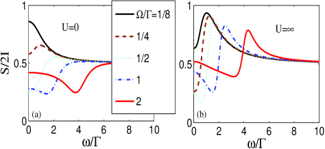
Figure 1: (Color online) Fano factor, $F=S(\omega)/2I$, vs. frequency, $\omega/\Gamma$, in a series-CQD for several values of dot-dot hopping strength, $\Omega/\Gamma=1/8$, $1/4$, $1/2$, $1$, and $2$, in the cases of absence of interdot Coulomb repulsion $U=0$ (a) and of strong Coulomb repulsion $U=\infty$ (b).

To start, we examine the noise spectrum of a series-CQD as it depends on increasing dot-dot hopping strength. The frequency-dependent Fano factor, $F=S(\omega)/2I$, is plotted as a function of normalized frequency $\omega/\Gamma$ in Figs. 1 and 2. Two rates are of essential importance in determining the noise spectrum: the rate of electrons entering into the system from the electrodes or its escape rate from the system, $\Gamma$; and the rate of coherent hopping between the two QDs, because electrons inside the system shuttle between the two QDs at a frequency $\Omega$. In the case of low hopping strength, $\Omega/\Gamma<1$, when an electron from the left lead is injected into the first QD, no further electrons can enter this QD until this electron transfers to the second QD with a quite long time scale, $\Omega^{-1}$, for this removal process. Thus, in this slow hopping limit, increasing $\Omega$ can enhance the transmission probability of an electron entering into the second dot, and thus reduce the zero-frequency shot noise (Fig. 1). As the frequency $\omega$ increases, the electron inside the first QD has a greater opportunity to instantly tunnel into the second QD, which enhances the shot noise. Consequently, the noise spectrum exhibits a nonzero-frequency peak as shown in Fig. 1. While, for high values of hopping strength, $\Omega/\Gamma>1$, the electron has a relatively high probability to enter into the second QD (once it is injected into the first QD from the left lead), it is also true that the electron also has high probability to return back to the first QD from the second QD periodically at a frequency $2\Omega$ (the Rabi frequency), before it escapes to the right lead, which takes place on a relatively long time scale determined by $\Gamma^{-1}$. The rapid return of the electron to the first dot blocks the entry of another electron into the dot, leading to a suppression of noise at $\omega=2\Omega$ in the absence of interdot Coulomb repulsion, as shown in Fig. 1(a) and 2(a). Similar noise properties were found in previous studies for a coupled double well structureSun and for a CQD.Djuric1

Figure 2: Noise spectrum for the right lead, $S_{R}(\omega)/2I$, the charge correlation spectrum, $S_{Q}(\omega)/2I$, and the Fano factor, $F=S(\omega)/2I$, vs. frequency, $\omega/\Gamma$, for a series-CQD with $\Omega/\Gamma=4$ in the cases of absence of interdot Coulomb repulsion $U=0$ (a) and of strong Coulomb repulsion $U=\infty$ (b).

Interestingly, we find that strong interdot Coulomb repulsion also plays a crucial role in determining noise. In Figs. 1(b) and 2(b), the noise spectrum exhibits a peak at $\omega=2\Omega$ for the system with strong dot-dot hopping and infinite Coulomb repulsion, instead of a dip for the system without interdot Coulomb repulsion. A similar Coulomb interaction effect on the noise spectrum was also reported for a single QD connected to two ferromagnetic electrodes.Gurvitz3 For the sake of comparison, we also plot the noise spectrum for the leads, $S_{R}(\omega)/2I$, and the charge correlation noise spectrum, $S_{Q}(\omega)/2I$, in Fig. 2. It is evident that Coulomb repulsion mainly influences noise in the leads, and it reduces the charge correlation spectrum by nearly a factor of $2$, but has little effect on its shape.

Moreover, strong dot-dot hopping strength, $\Omega$, combines the two dots rather tightly, and thus the CQD behaves much more like a single QD. As a result, the zero-frequency shot noise reduces to the result of a symmetric single QD, $F_{0}=1/2$ in the limit of $\Omega/\Gamma\rightarrow\infty$. This can be easily verified from Eqs. (14) and (37b) for $x\rightarrow\infty$. Strong Coulomb repulsion results in a bit larger Fano factor, $F_{0}=5/9$, from Eqs. (43) and (44b).

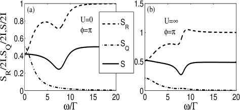
Figure 3: Noise spectrum for the right lead, $S_{R}(\omega)/2I$, the charge correlation noise spectrum, $S_{Q}(\omega)/2I$, and the Fano factor, $F=S(\omega)/2I$, vs. frequency, $\omega/\Gamma$, for a parallel-CQD with $\Omega/\Gamma=4$, $\Gamma^{\prime}/\Gamma=1$ and a magnetic-flux $\varphi=\pi$, in the cases of absence of interdot Coulomb repulsion $U=0$ (a) and of strong Coulomb repulsion $U=\infty$ (b).

We have also examined the quantum interference effect between the two distinct pathways of a CQD in a parallel arrangement on the noise power spectrum. We plot the frequency-dependent noise spectra for a completely symmetrical CQD interferometer ($\gamma=1$) with $x=\Omega/\Gamma=4$ at the magnetic-flux $\varphi=\pi$, in Fig. 3. It is evident from Fig. 3 that the noise spectrum of a parallel-CQD has similar properties as that of a series-CQD, i.e., has a dip at the Rabi frequency, in the absence of Coulomb interaction; but (2) it is different from a series-CQD in the presence of strong interdot Coulomb repulsion, i.e., it still exhibits a dip at the Rabi frequency.

To explore the quantum interference effect more fully, we analyze the noise spectrum as it depends on increasing tunneling strength, $\Gamma^{\prime}$, of the additional pathway. Figure 4 exhibits our numerical results for noise spectra with magnetic-fluxes, $\varphi=0$ and $\pi$, including the cases of no Coulomb repulsion and of strong Coulomb repulsion. It is clear that (1) increase of tunneling strength of the additional path branch continuously decreases the dip of the noise spectrum at $\omega=2\Omega$ if $\varphi=0$, while it continuously widens the dip if $\varphi=\pi$ for a system with no Coulomb repulsion [Figs. 4(a) and (b)]; (2) the combined effect of strong Coulomb repulsion and full interference gives rise to substantially enhanced zero-frequency noise, as pointed out previously in the absence of magnetic-flux,Dong4 but it decreases very rapidly to sub-Poissonian values at finite frequencies, and also its peak at $\omega=2\Omega$ is gradually suppressed by the interference effect [Fig. 4(c)]; and (3) the noise spectrum exhibits a transition peak–Fano-type structure–dip with increasing tunneling strength of the additional path branch for $\varphi=\pi$ [Fig. 4(d)].

Figure 4: (Color online) Fano factor, $F=S(\omega)/2I$, vs. frequency, $\omega/\Gamma$, for a CQD with $\Omega/\Gamma=4$ in the cases of absence of interdot Coulomb repulsion $U=0$ (a,b) and of strong Coulomb repulsion $U=\infty$ (c,d), as well as with different magnetic-fluxes, $\varphi=0$ (a,c) and $\varphi/\pi=1$ (b,d) for several values of additional tunneling strengths, $\Gamma^{\prime}/\Gamma=0$, $0.1$, $0.2$, $0.5$, and $0.8$.

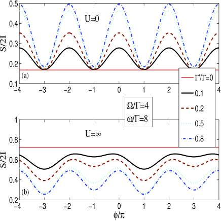
Figure 5: (Color online) Calculated Fano factor, $F=S(\omega)/2I$ at the Rabi frequency $\omega/\Gamma=8$, vs. magnetic-flux, $\varphi/\pi$, for various values of $\Gamma^{\prime}/\Gamma$ with $\Omega/\Gamma=4$ in the cases of absence of interdot Coulomb repulsion, $U=0$ (a), and of strong Coulomb repulsion, $U=\infty$ (b).

Finally, we exhibit the magnetic-flux dependence of the noise spectrum at $\omega=2\Omega$ (Fig. 5). It is evident that the noise spectrum is a periodic function of magnetic-flux, and the effect of strong Coulomb repulsion is to vary the period of the noise spectrum from $2\pi$ to $4\pi$.

VI Conclusions

In summary, we have analyzed the frequency-dependent current noise for coherent resonant tunneling through a CQD-AB interferometer in the case of an extremely high bias-voltage and zero temperature by means of number-resolved QREs and MacDonald’s formula. Our attention has been focused on the role of coherent dot-dot hopping as well as on the interference effect between two distinct path branches involving magnetic-flux dependence, and also on inter-dot Coulomb repulsion effects. We have derived explicit analytical expressions for noise power spectrum of a series-CQD and of a completely symmetric parallel-CQD for specific magnetic-fluxes, $\varphi=\pi$, in both cases of no inter-dot Coulomb interaction and of infinite inter-dot Coulomb repulsion. Our numerical calculations have shown that (1) in absence of Coulomb interaction, the noise spectrum of a series-CQD has a peak at the Rabi frequency for weaker dot-dot hopping, $\Omega/\Gamma<1$, but becomes an unambiguous dip for stronger dot-dot hopping, $\Omega/\Gamma\gtrsim 1$; (2) it always exhibits a peak due to Coulomb repulsion; and (3) this peak can gradually become a dip again for a parallel-CQD due to variation of interference pattern by tuning enclosed magnetic-flux.

References

• (1) Ya.M. Blanter and M. Büttiker, Phys. Rep. 336, 1 (2000).
• (2) C. Beenakker and C. Schönenberger, Phys. Today, May 2003, 37 (2003).
• (3) H.B. Sun and G.J. Milburn, Phys. Rev. B 59, 10748 (1999).
• (4) R. Aguado and T. Brandes, Phys. Rev. Lett. 92, 206601 (2004).
• (5) I. Djuric, Bing Dong, H.L. Cui, Appl. Phys. Lett. 87, 032105 (2005).
• (6) I. Djuric, Bing Dong, H.L. Cui, J. Appl. Phys. 99, 63710 (2006).
• (7) D. Mozyrsky, L. Fedichkin, S.A. Gurvitz, and G.P. Berman, Phys. Rev. B 66, 161313(R) (2002).
• (8) S.A. Gurvitz, D. Mozyrsky, and G.P. Berman, Phys. Rev. B 72, 205341 (2005).
• (9) A.W. Holleitner, C.R. Decker, H. Qin, K. Eberl, and R.H. Blick, Phys. Rev. Lett. 87, 256802 (2001).
• (10) A.W. Holleitner, R.H. Blick, A.K. Hüttel, K. Eberl, and J.P. Kotthaus, Science 297, 70 (2002).
• (11) J.C. Chen, A.M. Chang, and M.R. Melloch, Phys. Rev. Lett. 92, 176801 (2004).
• (12) T.V. Shahbazyan and M.E. Raikh, Phys. Rev. B 49, 17123 (1994).
• (13) D. Loss and E.V. Sukhorukov, Phys. Rev. Lett. 84, 1035 (2000); E.V. Sukhorukov, G. Burkard, and D. Loss, Phys. Rev. B 63, 125315 (2001).
• (14) J. König, and Y. Gefen, Phys. Rev. B 65, 45316 (2002).
• (15) B. Kubala, and J. König, Phys. Rev. B 65, 245301 (2002).
• (16) M.L. Ladrón de Guevara, F. Claro, and P.A. Orellana, Phys. Rev. B 67 195335 (2003).
• (17) Bing Dong, Ivana Djuric, H.L. Cui, and X.L. Lei, J. Phys.: Condens. Matter 16, 4303 (2004).
• (18) S.A. Gurvitz, IEEE Transactions on Nanotechnology, 4, 45 (2005).
• (19) Bing Dong and X.L. Lei, cond-mat/0611552 (2006).
• (20) D.K.C. MacDonald, Rep. Prog. Phys. 12, 56 (1948).
• (21) T.H. Stoof and Yu.V. Nazarov, Phys. Rev. B 53, 1050 (1996); B.L. Hazelzet, M.R. Wegewijs, T.H. Stoof, and Yu.V. Nazarov, Phys. Rev. B 63, 165313 (2001).
• (22) S.A. Gurvitz and Ya.S. Prager, Phys. Rev. B 53, 15932 (1996)
• (23) S.A. Gurvitz, Phys. Rev. B 57, 6602 (1998).
• (24) Bing Dong, H.L. Cui, and X.L. Lei, Phys. Rev. B 69 35324 (2004).
• (25) L.Y. Chen and C.S. Ting, Phys. Rev. B 46, 4714 (1992).
• (26) S. Ramo, Proc. IRE 27, 584 (1939); W. Schockley, J. Appl. Phys. 9, 639 (1938).
• (27) W. Shockley, J. Appl. Phys. 9, 639 (1938).
• (28) A.N. Korotkov, D.V. Averin, K.K. Likharev, and S.A. Vasenko, in Single-Electron Tunneling and Mesoscopic Devices, edited by H. Koch and H. Lübbig, Springer Series in Electronics and Photonics Vol. 31 (Springer-Verlag, Berlin, 1992), p. 45; A.N. Korotkov, Phys. Rev. B 49, 10381 (1994).
• (29) U. Hanke, Yu.M. Galperin, K.A. Chao and Nanzhi Zou, Phys. Rev. B 48, 17209 (1993).