Exact quantum Monte Carlo study of one dimensional trapped fermions with attractive contact interactions

Abstract

Using exact continuous quantum Monte Carlo techniques, we study the zero and finite temperature properties of a system of harmonically trapped one dimensional spin 1/2 fermions with short range interactions. Motivated by experimental searches for modulated Fulde-Ferrel-Larkin-Ovchinikov states, we systematically examine the impact of a spin imbalance on the density profiles. We quantify the accuracy of the Thomas-Fermi approximation, finding that for sufficiently large particle numbers ($N\gtrsim 100$) it quantitatively reproduces most features of the exact density profile. The Thomas-Fermi approximation fails to capture small Friedel-like spin and density oscillations and overestimates the size of the fully paired region in the outer shell of the trap. Based on our results, we suggest a range of experimentally tunable parameters to maximize the visibility of the double shell structure of the system and the Fulde-Ferrel-Larkin-Ovchinikov state in the one dimensional harmonic trap. Furthermore, we analyze the fingerprints of the attractive contact interactions in the features of the momentum and pair momentum distributions.

I Introduction

Mapping the phase diagram of fermions with attractive interactions and spin imbalance is a challenging problem, both from the experimental and the theoretical side. For an unpolarized system, an effective attractive interaction leads to the formation of Cooper pairs carrying zero momentum.cooper However in the presence of spin imbalance, where the different spin components have their Fermi energies shifted from one another, the pairing mechanism changes. Depending on parameters, different theories apply. The Sarma or breach-pair theory, which is stable in the presence of long range interactions, suggests a coherent superposition of Bardeen-Cooper-Schrieffer (BCS) pairs and normal fermions,sarma ; liu ; forbes ; gubbels while in other regimes one finds Fermi surface deformationsmuther ; sedrakian or a coexistence of normal fluid and superfluid.bedaque One of the most interesting possibilities is the Fulde-Ferrel-Larkin-Ovchinikov (FFLO) states,fulde ; larkin ; casalbuoni which reconcile spin imbalance and superconductivity by pairing particles whose momentum does not sum to zero. For example, in the FF state, $\uparrow$-spin fermions with momentum $k$ are paired with $\downarrow$-spin fermions with momentum $-k+q$, resulting in a Cooper pair with momentum $q$. In the LO theory, the Cooper pairs carry no net current, but are in superpositions of momentum states, leading to an order parameter that oscillates in space; the excess spin polarization resides in the nodes of the order parameter. Analogs of the latter state are found in one dimension (1D). We will use an exact quantum Monte-Carlo procedure to study a gas of spin imbalanced harmonically trapped 1D fermions, with a goal of identifying the signatures of FFLO physics which will be seen in cold atom experiments.

Although not completely transparent, the best evidence for the FFLO state in solid-state systems comes from layered organic superconductorssingleton and heavy-fermion materials.radovan ; miclea However, recent progress in optical lattice experiments with cold atoms has opened the avenue to study spin imbalanced fermions with attractive interactions in a clean and direct way. zwierlein ; zwierlein2 ; shin ; schunck ; partridge ; partridge2 Unfortunately, for a bulk three dimensional gas of atoms with short range interactions, the FFLO state is found for a very narrow range of chemical potentials,parish implying that only a small volume of a trapped atomic cloud would be in this state. Hence attention has been shifting to one dimension, where an analog of the FFLO state has a very large region of stability.liu_hu_drumm_fflo

Since there is no true off-diagonal long-range order in a strict 1D system, the 1D FFLO state is characterized by an algebraic quasi-1D order. Although the thermodynamics of a uniform 1D Fermi gas with contact interactions can be found exactly via the Bethe ansatz at zerogaudin ; takahashi and finite temperature,takahashi_temp ; guan the characterization of the ground state with spin imbalance is not easy: many correlation functions are unknown due to the complicated structure of the Bethe ansatz. Other properties are well known: for example, Yang firmly established the existence of the FFLO state through a bosonization technique, showing that it emerges via a continuous transition from the BCS state.jang Further, numerical methods have shown that the FFLO is the ground state of the Hamiltonian on a lattice as soon as the system is polarized batrouni ; rizzi ; luscher .

Experimentally, an array of quasi one dimensional tubes can be created at the intersection of two orthogonal standing waves generated by laser beams.paredes ; moritz ; moritz2 Along each tube there would be no lattice, but the particles will be confined by a longitudinal harmonic potential, coming from the spatial profile of the lattice lasers, and possibly from some additional potential. Recently Orsoorso and Liu at al.liu_hu_drumm_prl studied the properties of an atomic cloud in such a 1D harmonic trap. By using a Thomas Fermi (TF) approximation based on the Bethe ansatz solution of the homogeneous Hamiltonian, they found that in the trap the system phase separates. The inner shell of the tube is always a partially polarized FFLO state, while the outer shell can be either a fully paired BCS or a fully polarized normal state. Our calculations are designed to go beyond the approximations inherent in those calculations, and accurately quantify the properties of these 1D clouds.

Other researchers have also attempted to investigate the accuracy of the TF approximation. For example, Xianlong and Asgari developed an exchange-correlation functional to perform density functional theory (DFT) calculations with the local density approximation (LDA).xianlong While revealing, those calculations are only approximate. In a different direction, several researchers have used the density matrix renormalization group (DRMG) to study a related system, where there is a 1D lattice along the tube.feiguin ; tezuka ; capelle One needs to be cautious about applying those results to the continuous system as the underlying lattice in the model could introduce effects of incommensurability in the density profiles.buchler ; molina The continuous limit is difficult to access due to the large number of sites required in the DMRG evaluation for an extremely dilute system.

We will also consider how temperature affects the density profiles. Since the superfluid critical temperature is zero in 1D, thermal effects could be quite dramatic, and may not be captured by mean field theories.liu_hu_drumm_finitet Experiments will inevitably be performed at finite temperature, and it is imperative to know to what extent finite temperature will obscure the clear delineation of phases which are expected in a trapped zero temperature gas.

In this paper, we present exact results for 1D fermions subject to a zero-range attractive interaction and a longitudinal harmonic confinement. We resolve the dependence on the spin imbalance, effective coupling, and temperature, within a continuous quantum Monte Carlo (QMC) framework. We use diffusion Monte Carlo (DMC)reynolds:5593 for zero temperature ground state calculations and path integral Monte Carlo (PIMC)ceperley_pimc for finite temperature, which are ideal numerical tools to find the properties of 1D Hamiltonians, as they do not suffer from the “sign problem” which affects QMC simulations in higher dimensions.ceperley91 In 1D they give unbiased energies, with their accuracy only limited by statistical noise. We correct other potential errors in the DMC algorithm, such as the time step $\tau$, population bias, and mixed estimate errors, by appropriate extrapolation and forward walking techniques.calandra:1998 The only systematic bias in the PIMC algorithm is the time step, which we control by working with sufficiently small $\tau$.

The paper is organized as follows. In Sec. II we outline the model Hamiltonian used in our calculations, and the experimental parameters of the system. Sec. III includes a description of the QMC methods with an emphasis on the features required to simulate 1D fermions interacting with a zero-range potential. In Sec. IV we present our results and compare them with the TF findings. In particular, we focus our attention to the finite size and temperature effects on the phase boundaries. We conclude in Sec. V with some highlights and remarks.

II Model

The Hamiltonian which describes 1D fermions in a trap and interacting with an attractive zero-range potential is

$$H=-\frac{\hbar^{2}}{2m}\sum_{i=1}^{N}\frac{\partial^{2}}{\partial x_{i}^{2}}-g\sum_{i=1}^{N^{\uparrow}}\sum_{j=1}^{N^{\downarrow}}\delta(x_{i}-x_{j})+\frac{1}{2}m\omega_{z}^{2}\sum_{i=1}^{N}x_{i}^{2},$$ (1)

where $N=N^{\uparrow}+N^{\downarrow}$ is the total number of particles with mass $m$, $g(>0)$ is the strength of the contact interaction, and $\omega_{z}$ is the harmonic frequency of the longitudinal trap. The effective 1D Hamiltonian in Eq. 1 is a very good representation of a single tube in the optical array provided that $N\hbar\omega_{z}\ll\hbar\omega_{\perp}$ and $k_{B}T\ll\hbar\omega_{\perp}$, where $\omega_{\perp}$ is the frequency of the transverse harmonic confinement. The above requirements are met in the experimental setup by properly tuning the height of the lattice depth, which sets the value of $\omega_{\perp}$. In such a 1D geometry with just one open channel, the interactions can be modeled by as $V(x)=-g\delta(x)$ with $g$ given byolshanii ; bergeman

$$g=\frac{2\hbar^{2}a_{3D}}{ma^{2}_{\perp}}\frac{1}{Aa_{3D}/a_{\perp}-1},$$ (2)

where $a_{3D}$ is the 3D $s$-wave scattering length, $a_{\perp}=\sqrt{\hbar/m\omega_{\perp}}$ is the transverse oscillator length, and $A=-\zeta(1/2)/\sqrt{2}\simeq 1.0326$, where $\zeta$ is the Riemann zeta function. Here and throughout the paper we have used a sign convention where $g>0$ is attractive. An ongoing experiment at Rice Universityrandy is using $N\sim 100-300$ of ${}^{6}\textrm{Li}$ atoms per tube, the actual value depending on the position of the tube in the array. Typical values for the optical lattice are $\omega_{\perp}=2\pi~{}156~{}kHz$, $\omega_{z}=2\pi~{}200~{}Hz$, while $g$ will be tuned by changing $a_{3D}$. The typical temperatures are around $T\sim 0.05~{}T^{\uparrow}_{F}$, with $T^{\sigma}_{F}=N^{\sigma}\hbar\omega_{z}/k_{B}$ the Fermi temperature of fermions with spin $\sigma$. Throughout the paper we will use $m=\hbar=\omega_{z}=k_{B}=1$, i.e. the length will be measured in units of the harmonic oscillator length $\sqrt{\hbar/m\omega_{z}}$, and the energy and temperature in units of the level spacing $\hbar\omega_{z}$. In these units the energy for $g=0$ is $E=(N_{\uparrow}^{2}+N_{\downarrow}^{2})/2$ and the binding energy of a pair is $g^{2}/4$.

III Methods

The ground state QMC techniques used in this work are described in Subsec. III.1, while the finite temperature PIMC method is reported in Subsec. III.2. In order to compare our results with the local density approximation, we computed also the TF density profile ($n(x)=n^{\uparrow}(x)+n^{\downarrow}(x)$) and spin density profile ($s(x)=n^{\uparrow}(x)-n^{\downarrow}(x)$) of the system, which are solutions of:

$$\mu_{\textrm{hom},\sigma}[n(x),s(x)]+\frac{1}{2}x^{2}=\mu_{\sigma}\qquad\sigma=\uparrow,\downarrow,$$ (3)

where $\mu_{\sigma}$ is the chemical potential of the species with spin $\sigma$, and $\mu_{\textrm{hom},\sigma}$ is the local chemical potential found from the Gaudin exact solutiongaudin ; takahashi of the homogeneous model. The Thomas-Fermi results have been widely discussed elsewhere, and we refer the reader to previous worksorso ; liu_hu_drumm_prl ; liu_hu_drumm_fflo ; xianlong for complete details. Here, we mention that Eq. 3 can be rescaled into dimensionless variables with coupling strength controlled by $4N/g^{2}$. Therefore, the effective coupling constant of the trapped system depends also on the number of particles and scales as $g/\sqrt{N}$.

III.1 Ground state QMC

To study the ground state properties of the system, we employed variational and diffusion quantum Monte Carlo methods. Their basic ingredient is the trial wave function $\Psi_{T}$, a good approximation to the ground state. We used the form:

$$\Psi_{T}=D^{\uparrow}D^{\downarrow}\exp(-U),$$ (4)

where $U$ is a bosonic function and $D^{\sigma}$ is the antisymmetrized product of Hermite polynomials of $i$-th order $H_{i}$ for particles with spin $\sigma$. $D^{\sigma}$ can be written as determinant of a Van der Monde matrix:

$$D^{\sigma}(x_{1},\ldots,x_{N^{\sigma}})=\det(H_{i}(x_{j}))=\prod_{\begin{subarray}{c}1\leq i<j\leq N^{\sigma}\end{subarray}}(x_{i}-x_{j}).$$ (5)

The product in the Eq. 5 is convenient, as it can be evaluated in order $N_{\sigma}^{2}$ operations. The Hermite basis set yields an exact variational wavefunction in the limit of vanishing inter-particle interactions. The Slater term $D^{\uparrow}D^{\downarrow}$ determines the nodes of the variational wave function. In 1D, the exact nodes of the ground state are defined by the coalescence conditions between two like-spin particles (i.e. $x_{i}=x_{j}$ with $\sigma_{i}=\sigma_{j}$). This result holds even for an interacting system, and consequently there is no sign problem in the diffusion Monte Carlo calculations.ceperley91

The bosonic function $U$ is real and symmetric under permutation of two fermions, and is the sum of one-body ($U_{1b}$), two-body ($U_{2b}$), and three-body ($U_{3b}$) correlations. The one-body part reads:

$$U_{1b}=\sum_{i=1}^{N}f^{\sigma_{i}}(x_{i}),$$ (6)

where $\sigma_{i}$ is the spin of the $i$-th particle, and $f^{\sigma}(x)$ is written in a Padé form which goes as $x^{2}/2$ at large $x$ so to assure the right asymptotic behavior given by the harmonic confinement. In the absence of inter-particle interactions, $f^{\sigma}(x)=x^{2}/2$ is the exact solution.

The two-body (Jastrow) factor is defined as:

$$U_{2b}=\sum_{\begin{subarray}{c}1\leq i<j\leq N\end{subarray}}u^{\sigma_{i}\sigma_{j}}\left(x_{i}-x_{j}\right),$$ (7)

with $u^{\sigma_{i}\sigma_{j}}$ pair functions chosen to fulfill the cusp conditions set by the contact interactions of the Hamiltonian in Eq. 1. In the case of two unlike-spin particles interacting with a delta function potential, the exact solution is given by $\Psi(x^{\uparrow},x^{\downarrow})=\exp(-\frac{g}{2}|x^{\uparrow}-x^{\downarrow}|)$; note the cusp at $x^{\uparrow}=x^{\downarrow}$. The exact many-body function will have the same cusp between atoms with different spin. We use the following pair functions:

$$u^{\uparrow\downarrow}(x) = -\frac{g}{2\lambda}\exp\left(-\lambda|x|\right),$$ (8)

$$u^{\sigma\sigma}(x) = \alpha_{\sigma\sigma}\frac{\exp(-\beta_{\sigma\sigma}|x|)}{1+\exp(-2\beta_{\sigma\sigma}|x|)},\qquad\sigma\in\{\uparrow,\downarrow\},$$ (9)

where $\lambda$, $\alpha_{\sigma\sigma}$, and $\beta_{\sigma\sigma}$ are variational parameters, and $g$ is the strength of the contact interaction.

The confining potential leads to inhomogeneities that make it convenient to include an inhomogeneous Jastrow function:

$$U^{\textrm{non-homo}}_{2b}=\sum_{1\leq i<j\leq N}u^{\sigma_{i}\sigma_{j}}(x_{i}-x_{j})~{}f^{\sigma_{i}\sigma_{j}}(x_{i}+x_{j}),$$ (10)

where the pair function $u^{\sigma_{i}\sigma_{j}}$ is modulated by the function $f^{\sigma_{i}\sigma_{j}}$ which depends on the center of mass of the particles $x_{i}$ and $x_{j}$. The analytic form of $u^{\sigma\sigma^{\prime}}$ is the same as in Eq. 9 also for $\sigma\neq\sigma^{\prime}$, while $f^{\sigma\sigma^{\prime}}$ is chosen to be:

$$f^{\sigma\sigma^{\prime}}(x)=1+\gamma_{\sigma\sigma^{\prime}}\frac{\exp(-\delta_{\sigma\sigma^{\prime}}x)}{1+\exp(-2\delta_{\sigma\sigma^{\prime}}x)},$$ (11)

where $\gamma_{\sigma\sigma^{\prime}}$ controls the inhomogeneity. For $\gamma_{\sigma\sigma^{\prime}}=0$ one recovers the homogeneous case.

Finally, we employed a three-body term:

$$U_{3b}=\sum_{\begin{subarray}{c}i,j,k=1\end{subarray}}^{N}u^{\sigma_{i}\sigma_{j}}(x_{i}-x_{j})~{}u^{\sigma_{j}\sigma_{k}}(x_{j}-x_{k}),$$ (12)

where also in this case the functional form of $u$ is the same as in Eq. 9. We found this term important in the intermediate and strong coupling regime, when the local energy is dominated by the inter-particle potential.

Our variational ansatz includes about 30 parameters $\{p_{i}\}$, optimized by means of the stochastic reconfiguration algorithm,sorella:024512 ; casula:7110 which minimizes the total energy $E_{T}$ of the wave function with an iterative procedure based on the value of the forces, $-\partial E_{T}/\partial p_{i}$, acting on the parameters at each step. The optimal variational wave function is then projected to the ground state by using the diffusion Monte Carlo method (DMC)reynolds:5593 , which provides an unbiased estimate of the ground state energy. The physical observables, such as the charge and spin density profiles, are computed with the forward walking propagation of the mixed DMC distribution.liu74 ; calandra:1998

III.2 Finite temperature QMC

The finite temperature calculations are performed by using the path integral Monte Carlo (PIMC) methodceperley_pimc which is based on sampling the thermal density matrix $\rho(R,R^{\prime};\beta)$, with $\beta=1/k_{B}T$, $T$ the temperature, by means of a mapping of the quantum system into a classical system of polymers or Feynmanfeynman “paths”. $R\equiv\{x_{1},\ldots,x_{N}\}$ and $R^{\prime}\equiv\{y_{1},\ldots,y_{N}\}$ are all-particle configurations. During the Monte Carlo random walk the polymers are distributed according to the probability

$$\exp\left(-\sum_{m=1}^{M}S_{m}\right),$$ (13)

where the integration from $0$ to $\beta$ has been discretized into $M$ “time slices” of length $\tau=\beta/M$, $S_{m}=-\log\left[\rho(R_{m-1},R_{m};\tau)\right]$ is the action, and $R_{0}=R_{M}$. An accurate approximation of $\rho(R,R^{\prime};\tau)$ for the system under consideration is important to make the PIMC calculations feasible and efficient. In the case of the Hamiltonian in Eq. 1, $\rho(R,R^{\prime};\tau)$ can be written using a Trotter expansion as a product of four factors: the non-interacting ($\rho_{0}$), the harmonic ($\rho_{\textrm{harm}}$), the interacting ($\rho_{\textrm{int}}$), and the fermionic ($\rho_{\textrm{Fermi}}$). The non-interacting part corresponds to the propagator for free particles

$$\rho_{0}(R,R;\tau)=(2\pi\tau)^{-N/2}\exp\left\{-(R-R^{\prime})^{2}/2\tau\right\}.$$ (14)

We use the primitive approximationceperley_pimc to include the effect of the harmonic external potential:

$$\rho_{\textrm{harm}}(R,R^{\prime};\tau)=\exp\left\{-\frac{\tau}{4}\left(R^{2}+R^{\prime 2}\right)\right\}.$$ (15)

To account for the interactions we make use of the exact action for two particles in free space interacting with an attractive contact potential gaveau . In terms of the relative distances of the pair ($x_{\textrm{rel}}\equiv x_{1}-x_{2}$, $y_{\textrm{rel}}\equiv y_{1}-y_{2}$), the resulting propagator is:

$$\rho_{\delta}(x_{\textrm{rel}},y_{\textrm{rel}};\tau)= 1+\sqrt{\pi}s\exp\left\{s(s-2r)\right.$$ (16)

$$\left.+z^{2}(x_{\textrm{rel}}-y_{\textrm{rel}})^{2}\right\}\textrm{erfc}\left(r-s\right),$$

where $s=\frac{g}{2}\sqrt{\tau}$, $z=1/\sqrt{4\tau}$, $r=z\left(|x_{\textrm{rel}}|+|y_{\textrm{rel}}|\right)$. From this propagator, one obtains the many-body action by means of the pair-product approximationceperley_pimc

$$\rho_{\textrm{int}}(R,R^{\prime};\tau)=\prod_{i=1}^{N^{\uparrow}}\prod_{j=1}^{N^{\downarrow}}\rho_{\delta}(x_{i}-x_{j},y_{i}-y_{j};\tau),$$ (17)

where the product runs over all unlike-spin pairs. This, as the other approximations, becomes exact as $\tau\to 0$.

To include Fermi statistics into the PIMC method ceperley_fn the paths are constrained by the nodal regions, which act like barriers. Since the nodes are exactly known in 1D, and they do not depend on $\beta$, the restricted path integral formalism gives the exact result. An approximate fermion action is given by the image approximation:

$$\rho^{\sigma}_{\textrm{Fermi}}(R,R^{\prime};\tau)=\prod_{i=2}^{N^{\sigma}}\left(1-\exp\left\{\frac{(x_{i-1}-x_{i})(y_{i-1}-y_{i})}{2\tau}\right\}\right),$$ (18)

for each spin sector. It includes the nodes between neighboring particles as zero’s of the density matrix, and becomes exact in the $\tau=0$ limit. We assume that the like spins are ordered $x_{i-1}<x_{i}$ for $1<i\leq N_{\sigma}$.

The probability distribution in Eq. 13, based on the the density matrix $\rho_{\textrm{int}}(R,R^{\prime};\tau)$ defined above, is sampled via a generalized Metropolis algorithm. The paths are displaced with two types of moves: a multi-level bisection (level two and three have been used here) and a global move, which attempts to displace an entire polymer at once. When the convergence is reached, the thermal expectation values are computed as described in Ref. ceperley_pimc, .

IV Results

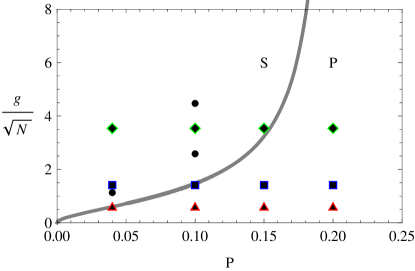
The QMC results shown in this section characterize the ground state and finite temperature properties of the system. We compute the density $n(x)$, spin density $s(x)$, and local polarization ($p(x)=s(x)/n(x)$) profiles. The latter quantity is extremely useful, as it locates the paired ($p=0$), partially polarized ($0<p<1$), and fully polarized ($p=1$) shells. For sufficiently high densities, the center of the cloud is always partially polarized, but the edge may be paired or fully polarized. The Thomas-Fermi approximation yields the phase diagram shown in Fig. 1, which shows the expected boundary between these two regimes. We decided to predominantly study the system with $N=200$, since it is roughly the average number of fermions per tube in typical experiments. As marked on the phase diagram, we present results for a range of interaction strengths and polarizations. In our numerical profiles we are particularly interested in how the visibility of the interface between different regions is influenced by finite particle number and finite temperature. By analyzing the experimental data within a Thomas-Fermi approximations one could use the locations of these boundaries to map out the phase diagram. We find that for $N\gtrsim 100$ and $T\lesssim 0.05T_{F}$ this Thomas-Fermi analysis is reasonable, but for fewer particles or higher temperatures one would need to use a much more sophisticated analysis of the experimental data to learn about the bulk zero temperature phase diagram. We report our results for the ground state and the finite temperature calculations in Secs. IV.1 and IV.2 respectively.

Figure 1: (Color online) Thomas-Fermi phase diagram in the polarization-coupling plane for 1D harmonically trapped cloud of two-component fermions, interacting through a contact potential $V(x_{i}-x_{j})=-g\delta(x_{i}-x_{j})$. The number of particles is $N$, the polarization $P$, and we use units where the harmonic confinement energy and length scales are set equal to unity. The gray thick line separates the phase region where the outer shell of the cloud is fully paired (S) from the region with fully polarized outer shell (P). The points locate our QMC simulations on the TF phase diagram. Triangles (red outline), squares (blue outline), and diamonds (green outline) refer to DMC data reported in Fig. 2, panels (a), (b), and (c) respectively. The two circles at $P=0.10$ depict systems with the same $g=20$ but different sizes ($N=60$ and $20$), displayed in Fig. 3. The circle at $P=0.04$ represents the system with $N=200$ and $g=16$, whose ground-state DMC polarization is reported in Fig. 4. At the same polarization, the triangle, circle and square points have been studied also by PIMC, which yielded temperature dependent polarizations reported in Figs. 8, 9, and 10 respectively.

IV.1 Ground state

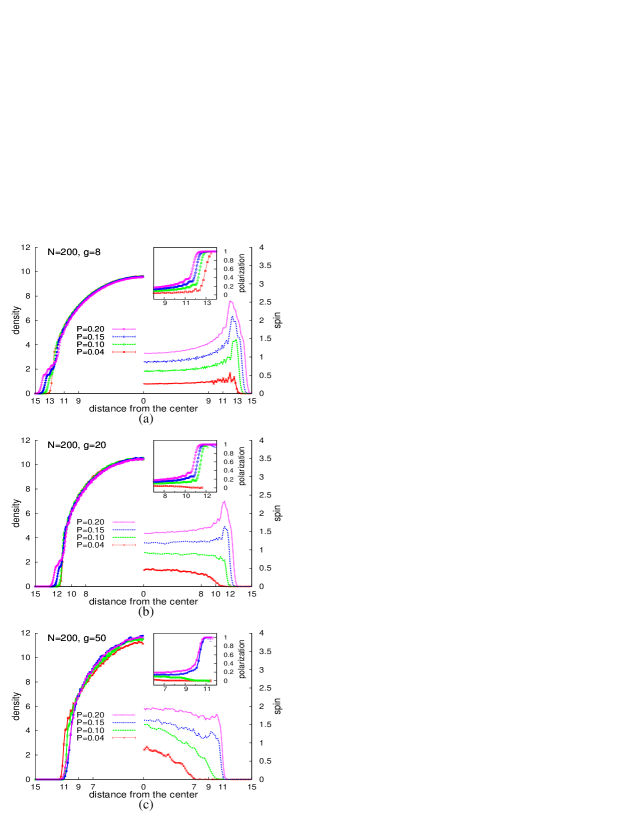
In Fig. 2 we report on the density, spin density, and local polarizations of $N=200$ particles with various polarizations $P$ and interaction strengths $g$. From the TF results in Fig. 1, one expects that the edge of the cloud will be fully polarized for $(g,P)=(8,0.2),(8,0.15),(8,0.1),(20,0.2),(20,0.15)$. Similarly, the edge should be fully paired for $(g,P)=(20,0.04),(50,0.1),(50,0.04)$. The others: $(g,P)=(8,0.04),(20,0.1),(50,0.15)$ are near-critical, and one expects that the FFLO state should extend nearly to the edge of the cloud. The results in Fig. 2 are consistent with these expectations. For the TF near-critical points, we found that all of them feature fully polarized wings. When the outer shell of the cloud is polarized, the spin density has a peak at the edge, which is replaced by a rapid fall-off when the edge is fully paired. Detecting the fully paired shell will be easiest at strong coupling, where the size of the outer paired region can be large.

Notice that the $g=50$ spin polarization plotted in Fig. 2(c) is much more noisy than for weaker interactions. Indeed, from the computational point of view a problem of ergodicity starts affecting the Monte Carlo (MC) sampling. As the coupling increases, one needs to run longer to equilibrate the sample and have good statistics in the expectation values, because sometimes the evolution gets stuck in a “persistent” configuration. In this regime, it is difficult for unpaired fermions to cross a strongly bound pair due to the Pauli principle. We note that it is possible that the same physics will affect also the dynamics of the ${}^{6}\textrm{Li}$ atoms in the experiment. The physical origin of the ergodicity problem in the MC evolution, namely the formation of strongly bound pairs, could also cause a slow equilibration in the experimental setup. A coupling between $g=20$ and $g=50$ is a good balance between the visibility of the fully paired region and the ergodicity of the pairs in the tubes.

Figure 2: (Color online) Density $n$, spin density $s$ and local polarization $p=s/n$ profiles for a cloud with $N=200$. The panel (a) shows the QMC results for $g=8$ and four different polarizations $P$, while panels (b) and (c) display the QMC density profiles for $g=20$ and $50$ respectively, with the same set of polarizations. The spin density is reported at the right side of the plot, while the density is on the left. The inset shows the polarization at the edge of the cloud, where the crossover from the FFLO core to the outer shell occurs. At $g=8$ the edge of the cloud is a completely polarized normal gas for all polarizations, whereas for $g=20$ and the lowest polarization $P$ the edge is in the fully paired state. At even stronger coupling ($g=50$), both $P=4\%$ and $P=10\%$ give fully paired outer shells. Finally, note how the strength of the interaction shrinks the cloud, while up to $P=20\%$ the polarization has a little impact on its spread. At $g=50$ the equilibration of the system begins to break down in the MC sampling, as particles are unable to easily cross each other, being the pairs strongly bound. This breakdown accentuates the MC noise in the results.

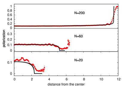
From the analysis presented above, it seems that the TF mean field phase diagram is a good approximation for the couplings and polarizations studied so far. It is clear that the TF approximation is not able to reproduce the short length-scale charge and spin fluctuations, since the local density approximation assumes a slow varying density profiles, as already pointed out in previous studies.mueller ; xianlong However, the TF boundaries of the phase separated states are in a quite good agreement with our exact QMC calculations. In order to better understand this agreement, we study the dependence of the local polarization on the number of particles $N$ and coupling $g$, and compare our QMC results with the TF predictions. The local polarization for different system sizes ($N=20$, $60$, $200$) with $g=20$ and $P=10\%$ is plotted in Fig. 3. At $N=20$ and $60$, there are qualitative disagreements between the QMC and TF methods, which disappears at $N=200$. Indeed for small systems our QMC calculations give partially polarized wings, while they are fully paired in the TF approximation. This can be due to a proximity effect not accounted for in the completely local TF approximation. We speculate that the FFLO state partially extends into the wings, making them partially polarized. We cannot confirm this picture since we did not study how the FFLO order parameter depends on position. For $N=200$ the wings become fully polarized, as the effective coupling is reduced, and the polarization profile turns out to be in agreement with the TF results, although the transition from the FFLO to the fully polarized state is much smoother in our QMC calculations. The boundaries between phase separated states are smeared out over a length-scale of order the atomic spacing. For small systems the very concept of phase separation begins to break down.

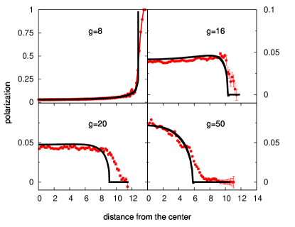
We check the agreement between the QMC and TF methods for large number of particles ($N=200$) in a more systematic way by studying the dependence of the polarization on $g$ with $P=4\%$. These results are plotted in Fig. 4 for $g=8$, $16$, $20$, and $50$. The TF polarization profile follows quite closely the DMC points. Both theories predict a “transition” from a fully polarized shell to a fully paired one between $g=8$ and $16$. Apart from fluctuations and statistical noise on the points, the only significant difference in the comparison is the size of the fully paired region which is smaller in the QMC results, where the FFLO state seems to extend farther from the center of the trap. This is a common feature of our calculations. The TF approximation always overestimates the size of the fully paired shell. Apparently, this is a drawback of the local density approximation, which makes the effective attractive interaction stronger.xianlong_lda

Figure 3: Local polarization profiles for $g=20$, $P=10\%$, and different number of particles $N$. The TF polarization is drawn (thick black line) for comparison. The TF approximation gives fully paired wings with zero polarization for $N=20$ and $60$, while the QMC polarization is always positive. The agreement between QMC and TF is better for the largest system ($N=200$), where the outer shell is fully polarized in both methods.

Figure 4: Local polarization profiles for $N=200$, $P=4\%$, at various couplings $g$. Also the TF polarization is drawn (thick black line) for comparison. The QMC results show a crossover to fully paired wings for $g\geq 16$, which is much smoother than the corresponding TF transition. Moreover, the QMC simulations give a larger partially polarized shell in the center of the trap.

We complete the comparison between the TF and QMC results by also computing the energetics of $g=20$ with different polarizations ($P=0\%$, $10\%$, $20\%$) and system sizes ($N=20$, $200$), reported in Tab. 1. The agreement in the ground state energies per particle between the two methods is remarkable, even at strong coupling (small $N$). This means that the total energy is insensitive to the local differences seen in the shell structure of the cloud, interpreted as finite size or edge effects. It also highlights the importance of an accurate treatment of local correlation effects, which can be missed in the TF approximation, and lead to subtle changes in the phase boundaries, whereas the overall trend is correctly captured by the mean field method, even at a quantitative level.

Table 1: Ground state energies per particle computed by means of DMC and TF, for $g=20$ at different polarizations ($P=0\%$, $10\%$, and $20\%$) and system sizes ($N=20$, and $200$).

$N$	$P$	TF energy	DMC energy
20	0%	$-47.265$	$-47.270(1)$
20	10%	$-42.550$	$-42.538(3)$
20	20%	$-37.587$	$-37.585(2)$
200	0%	$-35.731$	$-35.478(10)$
200	10%	$-13.991$	$-13.983(3)$
200	20%	$-7.914$	$-7.899(3)$

In previous works,batrouni ; tezuka ; feiguin ; rizzi it has pointed out that the pair momentum distribution function reveals fingerprints of the FFLO state in the center of the trap. The momentum and pair momentum distributions can be extracted in experiments from a statistical analysis of time-of-flight images of the expanding cloud of atoms when the confining potential is removed. Here we study the momentum distribution function defined as

$$n(k)=\int\,\mathrm{d}x\,\mathrm{d}y\rho(x,y)e^{ik(x-y)},$$ (19)

where $\rho(x,y)$ is the one-body density matrix

$$\rho(x,y)=\int\,\mathrm{d}x_{2}\cdots\,\mathrm{d}x_{N}\Psi(x,x_{2},\cdots,x_{N})\Psi(y,x_{2},\cdots,x_{N}),$$ (20)

and $\Psi$ is the ground state normalized such that

$$\int\,\mathrm{d}x\rho(x,x)=N.$$ (21)

In the actual DMC calculations, the density matrix in Eq. 20 is computed as follows

$$\rho(x,y)\approx\sum_{i=1}^{N}\left\langle\delta(x-x_{i})\frac{\Psi_{T}(\ldots,y,\ldots)}{\Psi_{T}(\ldots,x_{i},\ldots)}\right\rangle_{\textrm{MA}},$$ (22)

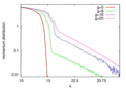
where $\langle\cdots\rangle_{\textrm{MA}}$ indicates the MC averages over $\{x_{1},\ldots,x_{i},\ldots,x_{N}\}$ sampled from the DMC mixed distribution. Although the forward walking technique for non-local operators is possible, it has rarely been applied to the evaluation of the momentum distributions.kalos In our case, we checked that the density matrix $\rho(x,y)$ computed at the variational MC level is close to the DMC mixed average (MA), due to the accuracy of the trial wave function $\Psi_{T}$. Therefore, our best estimate of $\rho(x,y)$ is a mixed average with a small bias. In Fig. 5 we plot $n(k)$ for different couplings and $N=200$. We found that the long-range tail of the momentum distribution decays as a power law as soon as the attractive contact interaction is switched on, and it is fitted well by $1/k^{4}$. This is the same behavior found by Minguzzi at al.minguzzi:2002 for the tail of the momentum distribution in a one dimensional gas of hard point-like bosons (Tonks gas) inside a harmonic trap. The power law decay is due to the cusp conditions of the wave function, a consequence of the attractive (or repulsive) contact interactions. The same decay has been shown recently by Santachiara and Calabrese for a one dimensional gas of impenetrable anyons.santachiara As one can see in Fig. 5, the momentum distribution does not discriminate between different phase separated states, but from the height of its tail one can get information on the effective interaction strength in the trap.

Figure 5: (Color online) Momentum distribution for $N=200$, $P=4\%$, at various couplings $g$, plotted in a log-log scale. Also the momentum distribution of the non interacting system is reported. The tails of the interacting $n(k)$ follow a straight lines with a slope compatible with a $1/k^{4}$ decay. Momenta are measured in units of $\sqrt{\hbar m\omega_{z}}$, where $\omega_{z}$ is the harmonic oscillator frequency along the tube. For comparison the characteristic momentum corresponding to the density at the center of the trap is $k_{F}=\pi/(2n)=16.5$ for $g=20$, while $k_{F}=14.1$ for the non-interacting system.

On the other hand, the pair momentum distribution carries fingerprints of the FFLO state. We define the pair two-body density matrix as

$$\rho_{\textrm{pair}}(x,y)= \int\,\mathrm{d}x_{3}\cdots\,\mathrm{d}x_{N}\Psi(x^{\uparrow},x^{\downarrow},x_{3},\cdots,x_{N})\times$$ (23)

$$\Psi(y^{\uparrow},y^{\downarrow},x_{3},\cdots,x_{N}),$$

where the pair $\{x^{\uparrow},x^{\downarrow}\}$ is chosen by selecting $x^{\uparrow}$ and finding $x^{\downarrow}$ as the position of the closest unlike-spin particle. $x$ ($y$) is the center of mass of the $\{x^{\uparrow},x^{\downarrow}\}$ ($\{y^{\uparrow},y^{\downarrow}\}$) pair. This is an unambiguous and generic way to define the pairs in a continuous system without introducing explicitly a characteristic length. Once $\rho_{\textrm{pair}}(x,y)$ is computed, the pair momentum distribution function $n_{\textrm{pair}}(k)$ is evaluated via Eq. 19, with $\rho(x,y)$ replaced by $\rho_{\textrm{pair}}(x,y)$. Also the normalization is based on the same formula as in Eq. 21, but with $N$ replaced by $N_{\textrm{pair}}$, i.e. the number of pairs in the system. The results for $n_{\textrm{pair}}(k)$ are presented in Fig. 6 for $g=20$, $N=200$, and various polarizations. A clearcut signature of the FFLO state is the presence of two peaks at $k=\pm|k^{\uparrow}_{F}-k^{\downarrow}_{F}|$, which signals a pairing with non zero total momentum given by the difference between the Fermi surfaces of up and down spin particles. Since the trap breaks the translational invariance, the Fermi momenta are approximated by $\tilde{k}^{\sigma}_{F}=\frac{\pi}{2}\frac{N^{\sigma}}{L}$, where $L$ is the effective spread of the cloud. The location of the peaks in Fig. 6 follows closely the relation $\pm|\tilde{k}^{\uparrow}_{F}-\tilde{k}^{\downarrow}_{F}|$.

Figure 6: (Color online) Pair momentum distribution (Fourier transform of the pair two-body density matrix in Eq. 23) for $g=20$, $N=200$, at various polarizations $P$. Momenta are measured in units of $\sqrt{\hbar m\omega_{z}}$, where $\omega_{z}$ is the harmonic oscillator frequency along the tube. The peaks of the pair momentum distribution are approximately given by $\pm|\tilde{k}^{\uparrow}_{F}-\tilde{k}^{\downarrow}_{F}|$, and are the signature of the FFLO state.

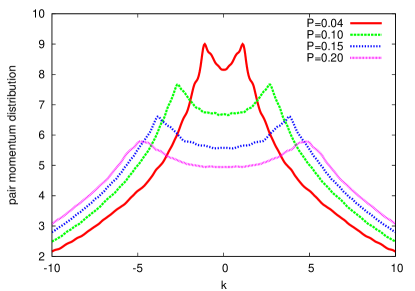
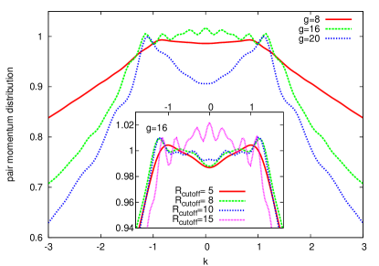
Fig. 7 displays the $n_{\textrm{pair}}(k)$ dependence on $g$ at fixed polarization $P=4\%$. At weak coupling ($g=8$) the peaks are short, and in the range $[-\tilde{k}^{\uparrow}_{F},\tilde{k}^{\downarrow}_{F}]$ the pair momentum distribution is almost flat. On the other hand, at $g=20$ the two peaks at $\pm|\tilde{k}^{\uparrow}_{F}-\tilde{k}^{\downarrow}_{F}|$ are taller, and the atoms in the cloud have a quite strong FFLO character. In the intermediate case analyzed here, namely $g=16$, the $n_{\textrm{pair}}(k)$ shows a fluctuating behavior, with peaks at $\pm|\tilde{k}^{\uparrow}_{F}-\tilde{k}^{\downarrow}_{F}|$ but also at $k=0$. By computing the Fourier transform (Eq. 19) of $\rho_{\textrm{pair}}(x,y)$ constrained in the region with $x,y\in[-R_{\textrm{cutoff}},R_{\textrm{cutoff}}]$ (and plotted in the inset of Fig. 7), we proved that the FFLO peaks come from the inner shell of the cloud, while the central peaks come from the wings. Indeed, around $g=16$ the system undergoes the transition from fully polarized to fully paired (BCS) wings (see Fig. 4). Both the FFLO pairing in the center and the BCS pairing in the outer shell are weak. Going from the center to the edge, the crossover between the two gives rise to this fluctuating pattern in the pair momentum distribution.

Figure 7: (Color online) Pair momentum distribution for $P=4\%$, $N=200$, at various couplings $g$. The functions have been rescaled such that the height of their peaks is around $1$ to make the comparison easier. The inset displays the pair momentum distribution for $g=16$ computed from $\rho_{\textrm{pair}}(x,y)$ with $x,y\in[-R_{\textrm{cutoff}},R_{\textrm{cutoff}}]$.

IV.2 Finite temperature

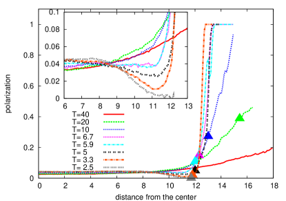
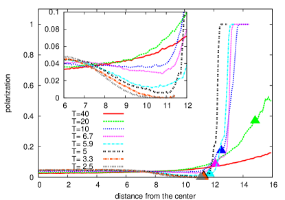
We performed finite temperature PIMC calculations for $g=8$, $16$, and $20$, with $P=4\%$, and $N=200$. From the DMC analysis and the TF results we know that for $g=8$ the phase separation is between an FFLO center and a fully polarized wing, while for $g=16$ and $20$ the outer shell is fully paired. Here we study how the phase separation evolves with the temperature.

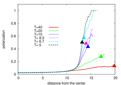
In Fig. 8 we plot the local polarization profile for $g=8$. At a temperature above $0.065~{}T^{\uparrow}_{F}$, the fully polarized shell becomes partially polarized with polarization progressively reduced as the temperature is raised. At $T\simeq 0.40~{}T^{\uparrow}_{F}$ the polarization is quite homogeneous throughout the cloud.

The finite temperature results at $g=16$ ($20$), reported in Fig. 9 (10), show a more complicated pattern. Up to a temperature of $T\simeq 0.06~{}T^{\uparrow}_{F}$ ($0.10~{}T^{\uparrow}_{F}$), the polarization profile has a dip around $x=11.5$ ($10.5$), which evolves into a fully paired region (with zero polarization) below $T\simeq 0.025~{}T^{\uparrow}_{F}$ ($0.035~{}T^{\uparrow}_{F}$). When the dip is present, the polarization in the outer part of the cloud increases until a fully polarized state occurs at the very edge of the cloud. This esternal region involves only $0.1\%$ of the atoms in the cloud, and so it will be hard to detect in the experiment. At higher temperatures, when the dip is gone, the fully polarized edge becomes unstable. For $T\simeq 0.40~{}T^{\uparrow}_{F}$ we have a situation analogous to the case with $g=8$, with a partially polarized state homogeneously spread over the cloud.

A feature common of all couplings is a crossover temperature $T_{c}$ above which the phase separation disappears and the whole cloud becomes partially polarized. This temperature depends on the polarization, since it scales roughly as $\mu^{\uparrow}-\mu^{\downarrow}$, whereas its dependence on the coupling is quite weak, at least until $g=20$. We found $T_{c}\simeq 0.065~{}T^{\uparrow}_{F}$ for $g=8$, and $T_{c}\simeq 0.10~{}T^{\uparrow}_{F}$ for $g=20$ with $P=4\%$. In case of fully polarized wings, one can define another critical temperature based on the stability of the pairs at the edge of the cloud. The fermions dissociate into a partially polarized fluid if the temperature is raised above a threshold proportional to $g^{2}$, as it depends on the binding energy of each pair.

As in the DMC calculations, the PIMC simulations suffer from the ergodicity problem mentioned before. This is an issue of the strictly one dimensional Monte Carlo sampling, where the exchange between particles or pairs is suppressed at strong coupling. For this particular system, we found that this issue is less severe in the DMC simulations than in the PIMC ones. Improved moves or working in the grand canonical ensemble could alleviate or solve the problem. Here, however, we could afford simulations with $N=200$ at quite strong coupling, namely up to $g=50$ in the DMC, and $g=20$ in the PIMC framework. Therefore our analysis has not been limited, since we were able to study the intermediate-strong coupling regime, where the fully paired region shows up at not-so-small polarizations.

Figure 8: (Color online) Local polarization profile for $N=200$, $P=4\%$, $g=8$, at various temperatures $T$ measured in units of $\hbar\omega_{z}$. For comparison, the central density in the trap corresponds to an energy $\epsilon_{F}=\hbar^{2}/2mk_{F}^{2}\simeq 229$. At this coupling the outer shell is fully polarized only at the two lowest temperatures considered here, while it becomes partially polarized at a temperature in between $T=7$ and $T=8$. The filled triangles indicate the polarization at the cloud radius which contains $99.9\%$ of atoms. The remaining $0.1\%$ ($0.2$ atoms) at the edge will be hard to detect in the experiment.

Figure 9: (Color online) Local polarization profile for $N=200$, $P=4\%$, $g=16$, at various temperatures $T$ measured in units of $\hbar\omega_{z}$. For comparison, the central density in the trap corresponds to an energy $\epsilon_{F}=\hbar^{2}/2mk_{F}^{2}\simeq 259$. The inset magnifies the region of the cloud around the polarization dip, where the pairing is the strongest. For temperatures above $2.5$ the fully paired region starts breaking. When a pair is broken, the unpaired fermions feel the difference in the chemical potential between the up and down species, resulting in the majority of up fermions at the edge of the trap, and a fully polarized outer shell. For even higher temperatures, the cloud becomes partially polarized everywhere. The filled triangles indicate the polarization at the cloud radius which contains $99.9\%$ of atoms.

Figure 10: (Color online) Local polarization profile for $N=200$, $P=4\%$, $g=20$, at various temperatures $T$ measured in units of $\hbar\omega_{z}$. For comparison, the central density in the trap corresponds to an energy $\epsilon_{F}=\hbar^{2}/2mk_{F}^{2}\simeq 272$. The inset magnifies the region of the cloud around the polarization dip, where the pairing is the strongest. At this stronger coupling, the fully paired region is more stable, and starts breaking at a higher temperature (above $T=3.5$ is this case). The filled triangles indicate the polarization at the cloud radius which contains $99.9\%$ of atoms.

V Conclusions

In this paper we have studied the properties of a system of 1D trapped fermions interacting via an attractive contact potential, by performing unbiased DMC and PIMC simulations. We showed that the trap induces the system to phase separate, in accordance to previous calculations done with the TF approximation.orso ; liu_hu_drumm_prl We compared the TF solution with our exact results, by studying their dependence on the coupling and system size. We found that the DMC phase boundaries are in a good agreement with the TF approximation for large number of particles ($N\gtrsim 100$) even at strong coupling. This is reasonable since the TF approach is applicable when $N\gg 1$, and the size of the cloud is large compared to the axial oscillator length. However, the local density approximation requires also a slow variation of the mean interparticle spacing, namely $\partial_{x}n(x)/n(x)^{2}\ll 1$, condition which is not fulfilled by the system particularly at the edge of the cloud, where the TF solution slightly overestimates the size of the outer fully paired region. For smaller systems we found that the agreement deteriorates. Indeed, at small $N$ a partially polarized state extends until the edge of the cloud even at intermediate coupling and small spin imbalance, in contrast with the TF approximation, which predicts a phase separation with fully paired wings.

As pointed out in a number of previous worksbatrouni ; tezuka ; feiguin ; rizzi the pair momentum distribution reveals the signature of the FFLO inner shell with two symmetric peaks centered at $\pm|k^{\uparrow}_{F}-k^{\downarrow}_{F}|$. It could be measured in the experiment by quickly removing the confining lattice and sweeping the magnetic field to the BEC side of the Feshbach resonance. This would bind the pairs into molecules, whose momentum distribution could be measured by means of time-of-flight imaging techniques.greiner The tails of the one-body momentum distribution strongly depend on the interaction strength and decay as $1/k^{4}$, due to the non analyticity of the exact wave function as a consequence of the delta function interaction. This could be another interesting quantity to measure in the experiment, although it does not carry information on the actual pairing in the system, but only on the effective strength.

The finite temperature PIMC calculations done with $N=200$, $P=4\%$, and three different couplings ($g=8$, $16$, and $20$) show a crossover from a phase separated state to a partially polarized state at $T\simeq 0.065~{}T^{\uparrow}_{F}$ for $g=8$, and $T\simeq 0.10~{}T^{\uparrow}_{F}$ for $g=20$. For the strongest coupling analyzed with this method ($g=20$), the fully paired region disappears already at $T\simeq 0.035~{}T^{\uparrow}_{F}$, leaving a dip in the polarization density profile which becomes shallower and shallower as the temperature increases. This quite low temperature (the experiments will access temperatures down to $T\simeq 0.05~{}T^{\uparrow}_{F}$) puts some limitation on the visibility of the fully paired phase at weak-intermediate coupling. One has to go to stronger coupling to make the pairs in the outer shell stable up to higher temperatures, being the binding energy proportional to $g^{2}$.

We discussed the ergodicity issues in the Monte Carlo sampling at strong coupling, and we identified the problem with the difficulty of unpaired fermions to pass through strongly bound pairs. The same slowing down in the equilibration might occur also in the experiment for ultra thin traps ($N\hbar\omega_{z}\ll\hbar\omega_{\perp}$ and $k_{B}T\ll\hbar\omega_{\perp}$). On the other hand, at weak coupling there are few particles involved in the fully paired region, which is very narrow, and the signal coming from this phase should be very difficult to detect in the experiment. We suggest that a good spot to detect the transition from the fully paired to the fully polarized state is for effective couplings $g/\sqrt{N}$ in the range $3-5$, where the system features a fully paired region up to $10\%$ of spin imbalance, the size of the two phase separated states is quite large, and the equilibration is not hard to reach.

The information coming from this paper could be combined with the recent work by Parish et al.,huse who studied the quasi one dimensional effects coming from the array of tubes in the transverse direction by means of a tight-binding model, in order to find out the parameters of the Hamiltonian which maximize the visibility of the FFLO state. In principle, one can extend the present work by explicitly including an array of tubes in the QMC simulations to study quasi one dimensional effects present in the experimental setup.