The Removal of Artificially Generated Polarization in SHARP Maps

Abstract

We characterize the problem of artificial polarization for the Submillimeter High Angular Resolution Polarimeter (SHARP) through the use of simulated data and observations made at the Caltech Submillimeter Observatory (CSO). These erroneous, artificial polarization signals are introduced into the data through misalignments in the bolometer sub-arrays plus pointing drifts present during the data-taking procedure. An algorithm is outlined here to address this problem and correct for it, provided that one can measure the degree of the sub-array misalignments and telescope pointing drifts. Tests involving simulated sources of Gaussian intensity profile indicate that the level of introduced artificial polarization is highly dependent upon the angular size of the source. Despite this, the correction algorithm is effective at removing up to 60% of the artificial polarization during these tests. The analysis of Jupiter data taken in January 2006 and February 2007 indicates a mean polarization of $1.44\%\pm 0.04\%$ and $0.95\%\pm 0.09\%$, respectively. The application of the correction algorithm yields mean reductions in the polarization of approximately 0.15% and 0.03% for the 2006 and 2007 data sets, respectively.

1 Introduction

Submillimeter polarimetry provides a means to investigate the morphology of interstellar magnetic fields that are highly embedded in dusty clouds. Such an investigative tool is extremely useful for the study of astrophysical phenomena in which magnetic fields are suspected to play a significant role. Such areas of interest include: star formation (Shu, Adams, and Lizano, 1987; Hildebrand, Dragovan, and Novak, 1984), circumstellar disks and jets (Davis et al., 2000), filamentary structure in molecular clouds (Fiege and Pudritz, 2000), and galactic-scale field morphology (Greaves and Holland, 2002). In the particular case of low mass star formation, the current leading model places great emphasis upon the presence of embedded magnetic fields to regulate the entire process (Mouschovias, 2001). Hence any further understanding of these magnetic fields may yield a clearer understanding of the origins of “solar-like” stellar/planetary systems.

Current work in this field is being carried out at the Caltech Submillimeter Observatory (CSO) using the Submillimeter High Angular Resolution Polarimeter (SHARP). SHARP is a fore-optics module designed to be used in conjunction with the SHARC-II camera to form a highly sensitive, dual-wavelength (350-$\mu\mathrm{m}$ and 450-$\mu\mathrm{m}$), polarimeter (Novak et al., 2004; Li et al., 2006). SHARC-II employs a 12 $\times$ 32 pixel bolometer array that is optically “split” by SHARP into three zones: two 12 $\times$ 12 pixel regions that record orthogonal states of linear polarization (which are labeled “H” and “V” for horizontal and vertical, respectively), and a 12 $\times$ 8 pixel central zone that is not used with SHARP. The horizontal and vertical components are combined during data reduction to yield the $I$, $Q$, and $U$ Stokes parameters.

The simultaneous measurement of the H and V polarization components allows for the effective removal of the sky background signal (Hildebrand et al., 2000). However, it does not negate the possibility of erroneous polarization signal generation. The combination of misalignments between the two sub-arrays (i.e., H and V) and pointing drifts during the observation cycle, can result in the generation of artificial polarization. The generation of these erroneous signals may place limitations on the sensitivity of SHARP and thus could reduce data-gathering efficiency. This would hurt efforts to rapidly survey large extended objects, such as giant molecular clouds (GMC’s), where many observations would be required to properly survey the source and thus a high data-taking efficiency is required.

A correction algorithm has been designed in an attempt to model and correct for this problem in the SHARP data reduction pipeline. This paper will go over in detail the problem of artificial polarization in dual-array polarimeters and the algorithm by which a correction is attempted, with simulated and planetary data being used to test the proposed method. Section 2 will describe the means by which artificial polarization is generated in a dual-array polarimeter. Section 3 will describe the algorithm employed to treat this problem. Section 4 of this paper will discuss the magnitude of the problem and cover the results obtained thus far from the testing of simulated and planetary data. Section 5 covers the concluding remarks.

2 Artificial Polarization

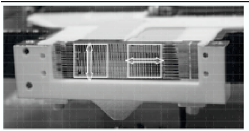
Figure 1: The SHARC-II bolometer array. The outlined squares with arrows indicate the vertical (V) and horizontal (H) sub-arrays. The central region is a dead zone (from Li et al. 2006).

Figure 1 illustrates how the SHARC-II array is segmented into three regions; the aforementioned “H” and “V” sub-arrays for the horizontal and vertical polarization components, respectively, and a central unused zone. Note that horizontal and vertical are defined with respect to the long axis of the bolometer array, which in the case of Figure 1 is the axis parallel to the horizontal of the image. Consider the radiation beam that is incident to the H and V sub-arrays. This radiation beam originates from a single patch of sky that is subsequently “split” into two components; a horizontally polarized component and a vertically polarized component (Novak et al., 2004). As the name sake would suggest, the optical path of SHARP is designed such that the horizontally polarized component is incident on the “H” sub-array while the vertically polarized component is incident on the “V” sub-array. In this way, both arrays image the same patch of sky. Also consider two position vectors, $\mathbf{x_{\mathrm{H}}}$ and $\mathbf{x_{\mathrm{V}}}$, that we will use to map the H and V sub-arrays, respectively. Note that each of these vectors has an independent origin (in their respective sub-arrays). Once the incident radiation is absorbed by the bolometers, we can express the resultant flux as being a function of the position vectors for both the H and V sub-arrays, $f_{\mathrm{H}}(\mathbf{x_{\mathrm{H}}})$ and $f_{\mathrm{V}}(\mathbf{x_{\mathrm{V}}})$ , respectively.

Now the two position vectors will be related through:

$$\mathbf{x_{\mathrm{V}}}=\mathbf{d}+\mathbf{R}\mathbf{S\mathbf{x_{\mathrm{H}}}},$$ (1)

where the quantities $\mathbf{d}$, $\mathbf{R}$, and $\mathbf{S}$ are the V array translational displacement, rotation, and stretch matrices relative to the H array, which is taken as a reference. Note that the stretch matrix describes a magnification/minification of the image on the sub-array. In an ideal setting we would have: $\mathbf{d}=\mathbf{0}$, $\mathbf{R}=\mathbf{1}$, and $\mathbf{S}=\mathbf{1}$ where $\mathbf{0}$ is a “zero” vector and $\mathbf{1}$ is the identity matrix. This would imply no array misalignments and $\mathbf{x_{\mathrm{H}}}=\mathbf{x_{\mathrm{V}}}=\mathbf{x}$. As will be explained later, in this case any measured polarization would result from either: 1) the detection of a polarized source or, 2) instrumental polarization. In reality, however, small misalignments between the arrays are present and complicate the interpretation of the polarization data.

During one cycles-worth of observations, measurements of $f_{\mathrm{H}}(\mathbf{x_{\mathrm{H}}})$ and $f_{\mathrm{V}}(\mathbf{x_{\mathrm{V}}})$ are made for each of the four half wave plate (HWP) angular positions: $\theta=0^{\circ},\,22.5^{\circ},\,45^{\circ},\,$ and $67.5^{\circ}$. The effect of rotating the HWP is to rotate the polarization of the incoming signal by $2\theta$ (Hildebrand et al., 2000). This enables the flux of the signal to be measured with its incident state of linear polarization rotated by angles of $\;0^{\circ},\,45^{\circ},\,90^{\circ},\,135^{\circ}$ and thus allows for the calculation of the Stokes parameters. Note that only the linear polarization can be determined with this methodology, as measurements of circular polarization would require the use of a quarter wave plate. What is obtained in the end are eight flux maps, four H array maps and four V array maps, that can then be processed to generate images of the Stokes parameters $I$, $Q$, and $U$. These parameters are given by:

$$I = \frac{1}{4}\{f_{\mathrm{H}}(\mathbf{x_{\mathrm{H}}^{\mathrm{0^{\circ}}}})+f_{\mathrm{V}}(\mathbf{x_{\mathrm{V}}^{\mathrm{0^{\circ}}}})+f_{\mathrm{H}}(\mathbf{x_{\mathrm{H}}^{\mathrm{22.5^{\circ}}}})+f_{\mathrm{V}}(\mathbf{x_{\mathrm{V}}^{\mathrm{22.5^{\circ}}}})\}$$ (2)

$$+\frac{1}{4}\{f_{\mathrm{H}}(\mathbf{x_{\mathrm{H}}^{\mathrm{45^{\circ}}}})+f_{\mathrm{V}}(\mathbf{x_{\mathrm{V}}^{\mathrm{45^{\circ}}}})+f_{\mathrm{H}}(\mathbf{x_{\mathrm{H}}^{\mathrm{67.5^{\circ}}}})+f_{\mathrm{V}}(\mathbf{x_{\mathrm{V}}^{\mathrm{67.5^{\circ}}}})\}$$

$$Q = \frac{1}{2}\{[f_{\mathrm{H}}(\mathbf{x_{\mathrm{H}}^{\mathrm{0^{\circ}}}})-f_{\mathrm{V}}(\mathbf{x_{\mathrm{V}}^{\mathrm{0^{\circ}}}})]-[f_{\mathrm{H}}(\mathbf{x_{\mathrm{H}}^{\mathrm{45^{\circ}}}})-f_{\mathrm{V}}(\mathbf{x_{\mathrm{V}}^{\mathrm{45^{\circ}}}})]\}$$ (3)

$$U = -\frac{1}{2}\{[f_{\mathrm{H}}(\mathbf{x_{\mathrm{H}}^{\mathrm{22.5^{\circ}}}})-f_{\mathrm{V}}(\mathbf{x_{\mathrm{V}}^{\mathrm{22.5^{\circ}}}})]-[f_{\mathrm{H}}(\mathbf{x_{\mathrm{H}}^{\mathrm{67.5^{\circ}}}})-f_{\mathrm{V}}(\mathbf{x_{\mathrm{V}}^{\mathrm{67.5^{\circ}}}})]\},$$ (4)

where $\mathbf{x_{\mathrm{i}}^{\theta}}=\mathbf{\mathrm{\mathbf{x}}_{\mathrm{i}}}+\mathbf{p^{\theta}}$ with $\theta=22.5^{\circ},\,45^{\circ},\,$ and $67.5^{\circ}$ for the HWP angles, and $\mathbf{\mathrm{i\,}}$= {H,V}. The $\mathbf{p^{\theta}}$ vectors represent the mean telescope pointing drift at the $\theta$ HWP angle with respect to the reference $\mathbf{p^{\mathrm{0}}}=\mathbf{0}$ . This implies that we must treat the flux as being a function of $\theta$, as well as position on the sub-arrays; this is included in the notation of equations (2), (3), and (4). Ideally, observations would not suffer from pointing errors and thus $\mathbf{p}^{\theta}=\mathbf{0}$ , regardless of the HWP angle. However, in reality the pointing will drift by some amount over the course of the cycle. Note that the nature of this pointing drift is random, systematic shifts in the telescope pointing over the course of one modulation cycle.

We are now in a position to study the root causes of artificial polarization. For the purpose of this illustration let us assume we are dealing with an unpolarized source. If misalignments exist between the H and V arrays such that the pixel space coordinates between the two sub-arrays are related by equation (1), then for any position on the array the quantity $T$:

$$T(\mathbf{x}_{\mathrm{H}}^{\theta},\mathbf{x_{\mathrm{\mathrm{V}}}^{\theta}})\equiv f_{\mathrm{H}}(\mathbf{x}_{\mathrm{H}}^{\theta})-f_{\mathrm{\mathrm{V}}}(\mathbf{x}_{\mathrm{V}}^{\theta})$$ (5)

will be non-zero. However, since each expression for $Q$ and $U$ contains the difference (denoted as $M$) between such terms:

$$M\equiv T(\mathbf{x}_{\mathrm{H}}^{\theta},\mathbf{x_{\mathrm{\mathrm{V}}}^{\theta}})-T(\mathbf{x}_{\mathrm{H}}^{\theta+45^{\circ}},\mathbf{x_{\mathrm{\mathrm{V}}}^{\theta+\mathrm{45^{\circ}}}}),$$ (6)

then these non-zero values will cancel each other out provided there is no pointing drift, $\mathbf{p^{\theta}}$, between HWP positions. This is due to our assumption that the signal is unpolarized.

If a pointing drift is present, each $f_{\mathrm{i}}(\mathbf{x}_{\mathrm{i}}^{\theta})$ term (where $\mathrm{i}$ = {H,V}) in equations (2), (3), and (4) would represent the flux of the source offset with respect to the reference position at $\theta=0^{\circ}$. The presence of these offsets between HWP positions could prevent the cancellation in equation (6) of the non-zero difference terms in equation (5) originating from array misalignments. Only if the source flux $f_{\mathrm{i}}(\mathbf{x}_{\mathrm{i}}^{\theta})$ has a linear gradient over the image (or none at all, in which case we would be dealing with a flat field) will the combination of array misalignments plus pointing drifts cause no artificial polarization. This is because $M=0$ for sources with linear gradients regardless of any pointing drifts or array misalignments that may be present during data collection.

In the most general case however, the source fluxes $f_{\mathrm{i}}(\mathbf{x}_{\mathrm{i}}^{\theta})$ will have non-linear gradients over the array, and pointing drifts and misalignments will be present. In this case there is nothing to prevent the Stokes $Q$ and $U$ parameters from acquiring non-zero values for some positions, even if the instrumental polarization is fully removed from the data and the source is completely unpolarized.

3 Algorithm for Corrections

We begin by first assuming that the values for $\mathbf{d}$, $\mathbf{R}$, $\mathbf{S}$, and $\mathbf{p^{\theta}}$ are known. Section 4.1 will briefly discuss how these quantities are actually measured with SHARP. To remove the artificial polarization from the data, the array misalignments and pointing drifts that would normally distort the H and V maps must be corrected. Consider an arbitrary position vector $\mathbf{a}$ specifying a position on a given source. The goal here is to setup the corresponding position vectors ($\mathbf{a_{\mathrm{H}}}$ and $\mathbf{a_{\mathrm{V}}}$) for the sub-arrays. This is illustrated below in equations (7) and (8):

$$\mathbf{a_{\mathrm{H}}^{\theta}} = \mathbf{a-p^{\theta}}$$ (7)

$$\mathbf{a_{\mathrm{V}}^{\theta}} = \mathbf{S^{\mathrm{-1}}R^{\mathrm{-1}}(a-d-p^{\theta})},$$ (8)

where $\mathbf{RR^{\mathrm{-1}}=\mathbf{1}}$ and $\mathbf{SS^{\mathrm{-1}}=\mathbf{1}}$. Now the flux measured on the two sub arrays at the positions corresponding to $\mathbf{a}$ can be expressed as:

$$H(\mathbf{a},\theta) = f_{\mathrm{H}}(\mathbf{a}_{\mathrm{H}}^{\theta})$$ (9)

$$V(\mathbf{a},\theta) = f_{\mathrm{V}}(\mathbf{a_{\mathrm{V}}^{\theta}}).$$ (10)

The fluxes $H(\mathbf{a},\theta)$ and $V(\mathbf{a},\theta)$ are now used to compute $Q$ and $U$ maps that are free of artificial polarization :

$$I(\mathbf{a}) = \frac{1}{4}\{H(\mathbf{a},0^{\circ})+V(\mathbf{a},0^{\circ})+H(\mathbf{a},22.5^{\circ})+V(\mathbf{a},22.5^{\circ})\}$$ (11)

$$+\frac{1}{4}\{H(\mathbf{a},45^{\circ})+V(\mathbf{a},45^{\circ})+H(\mathbf{a},67.5^{\circ})+V(\mathbf{a},67.5^{\circ})\}$$

$$Q(\mathbf{a}) = \frac{1}{2}\{[H(\mathbf{a},0^{\circ})-V(\mathbf{a},0^{\circ})]-[H(\mathbf{a},45^{\circ})-V(\mathbf{a},45^{\circ})]\}$$ (12)

$$U\left(\mathbf{a}\right) = -\frac{1}{2}\{[H(\mathbf{a},22.5^{\circ})-V(\mathbf{a},22.5^{\circ})]-[H(\mathbf{a},67.5^{\circ})-V(\mathbf{a},67.5^{\circ})]\}.$$ (13)

4 Results

This section is subdivided into three portions; a brief description of the observed hardware misalignments and pointing drifts, the degree to which artificial polarization affects polarimetry data, and results from simulated and planetary data.

4.1 Measured Hardware Misalignments and Pointing Drifts

The stretches, rotation angles, and translations of the H and V SHARC-II bolometer sub-arrays can be measured by placing an opaque plastic disk in the optical path before SHARP with five pinholes drilled through it. The pinholes are arranged in a “cross-pattern” with the central hole approximately aligned with the middle of the sub-arrays and the remaining four holes placed equidistantly from this central position. Data taken with this disk in place and a uniform background source (e.g., a cold load) can be analyzed to yield the hardware misalignments. For observing runs where no alignment data is taken with the opaque disk, the translations $\mathbf{d}$ can still be measured by comparing the centroid positions of images on the sky (e.g., for Jupiter observations) in the H and V sub-arrays. Typical values include a negligible stretch and a relative rotation of $\thickapprox 2^{\circ}-3^{\circ}$. During the two periods in which the planetary data to be discussed later were taken, the translational misalignments were measured to be:

$$(d_{x}\pm\delta d_{x},d_{y}\pm\delta d_{y}) = (-0.45\pm 0.07,-0.11\pm 0.04)\,\mathrm{pixels}\,\mathrm{[January\,2006]}$$ (14)

$$(d_{x}\pm\delta d_{x},d_{y}\pm\delta d_{y}) = (-0.02\pm 0.12,-0.41\pm 0.05)\mathrm{\,pixels}\,\mathrm{[February\,2007]},$$ (15)

where $d_{x}$ and $d_{y}$ are directed along the horizontal and vertical axes of the bolometer, respectively. Note that negative signs imply the V sub-array is shifted to the right, or down, of the H sub-array for an observer looking along the SHARP optical path towards the bolometer array. The net maximum translation is calculated to be approximately $\thickapprox 0.47$ and $\thickapprox 0.43$ pixels for the 2006 and 2007 observing runs, respectively. This net maximum translation is calculated by adding in quadrature the horizontal and vertical means and standard deviations.

The pointing drifts are measured via a correlation program that analyzes the intensity maps for a given source at each of the four HWP positions sequenced through during a cycle. The intensity map at $\theta=0^{\circ}$ is taken as the reference for this analysis. The results vary with each observing run and weather conditions. However, the mean pointing drifts measured in January 2006 and February 2007 are:

$$(p_{x}\pm\delta p_{x},p_{y}\pm\delta p_{y}) = (0.03\pm 0.20,0.01\pm 0.10)\mathrm{\,pixels}\,\mathrm{[January\,2006]}$$ (16)

$$(p_{x}\pm\delta p_{x},p_{y}\pm\delta p_{y}) = (0.01\pm 0.12,-0.02\pm 0.10)\,\mathrm{pixels}\,\mathrm{[February\,2007]},$$ (17)

where $p_{x}$ and $p_{y}$ are directed along the horizontal and vertical axes of the bolometer, respectively. It is apparent that there is a considerable spread about the mean drift magnitude. The net maximum pointing drift is thus calculated to be $\thickapprox 0.23$ and $\thickapprox 0.16$ pixels per HWP position for the 2006 and 2007 observing runs, respectively. This net maximum pointing drift is calculated by adding in quadrature the horizontal and vertical means and standard deviations. Each HWP position requires approximately 1.81 minutes of integration time when using SHARP.

4.2 A Measure of the Artificial Polarization Problem

Simulated data are generated as Gaussian sources with various elliptical aspect ratios. In addition to this, artificial hardware misalignments and pointing drifts can be introduced into the data. For the purpose of this discussion three unpolarized simulated sources were generated: a 9″circular, a 20″circular, and a 10″$\times$ 15″elliptical Gaussians (note that one SHARP pixel is approximately 4.6″$\times$ 4.6″). These dimensions refer to the Full-Width-Half-Magnitudes (FWHM) of the source. These data were generated with no bad pixels in the array and no noise. The sources were subjected to a range of hardware misalignments and pointing drifts. The results are presented in Figure 2.

It should be noted that in our simulation software the pointing drifts are introduced into the data cycle by selecting a magnitude $m$ and direction represented by a unit vector $\mathbf{e}_{i}$. Then for each HWP position ($\theta=0^{\circ},\,22.5^{\circ},\,45^{\circ},\,67.5^{\circ}$) the following drifts were introduced into the data: $0$, $m\mathbf{e}_{i}$, $2m\mathbf{e}_{i}$, and $-m\mathbf{e}_{i}$, respectively. This is hardly a random pointing drift; in fact each displacement lies on a line defined by the unit vector $\mathbf{e}_{i}$. Therefore it is easy to conclude that our modeling of the pointing drift has limitations when compared with the random, systematic drifts that are present in real data.

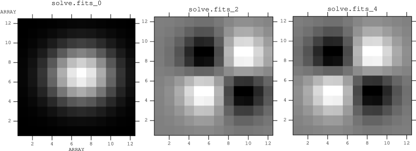
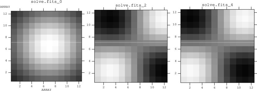
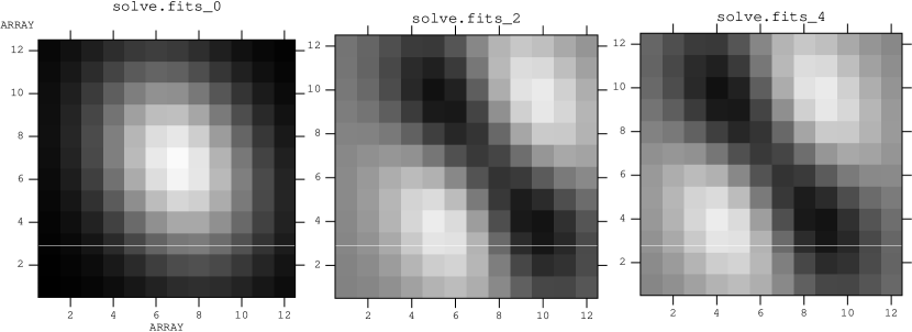
Figure 3: The $I$, $Q$, and $U$ maps (from left to right) for the 9″circular (top row), 20″circular (middle row), and 10″$\times$ 15″elliptical (bottom row) Gaussian sources. To generate the images presented here a pointing drift of 4.6 arcseconds per HWP position (in the horizontal direction) and a translational misalignment between the H and V sub-arrays of 0.5 pixels (in the vertical direction) were applied to the simulations. Remember that one SHARP pixel length is equivalent to 4.6 arcseconds. For the 9″circular source, the $I$ map grey levels are at a linear scale of 0 to 1.7 (from black to white) arbitrary data units, while the $Q$ and $U$ maps are at a linear scale of -0.04 to 0.04 (from black to white) data units. For the 20″circular source, the $I$ map grey levels are at a linear scale of 0 to 1.9 (from black to white) data units, while the $Q$ and $U$ maps are at a linear scale of -0.01 to 0.01 (from black to white) data units. For the 10″$\times$ 15″elliptical source, the $I$ map grey levels are at a linear scale of 0 to 1.8 (from black to white) data units, while the $Q$ and $U$ maps are at a linear scale of -0.03 to 0.03 (from black to white) data units.

One notices immediately the varying magnitude of the artificial polarization illustrated over the three plots. The 9″circular Gaussian generates roughly 8% of artificial polarization for a 0.5 pixel translation and a pointing drift of one SHARP pixel (i.e., 4.6″) per HWP position, while the 20″circular Gaussian generates only about 0.4% for the same misalignments and drifts. This trend is directly related to the broadness of the source; a more compact source will have a larger intensity gradient across its profile and as such a large polarization is induced due to the abrupt change in intensity with position. To understand this effect better it is instructive to compare the actual maps of the Stokes parameters $I$, $Q$, and $U$ for these simulated sources. These are presented in Figure 3 for the case of a 4.6 arcseconds per HWP position pointing drift (in the horizontal direction) and a 0.5 pixel translation between the H and V sub-arrays (in the vertical direction). The alternating light-dark pattern seen in the $Q$ and $U$ images results from the fact that the pointing drift and array translation are in orthogonal directions, and from the shape of the source itself. The $Q$ and $U$ images look identical as the simulated source is unpolarized. As a result, equations 3 & 4 will have no dependance on the HWP angle and are thus mathematically equivalent. One should note that the maps of $Q$ and $U$ illustrated in this figure would be flat, uniform fields if no artificial linear polarization were detected from any of the sources. The results are contrary to this however, with structure being apparent in the $Q$ and $U$ maps for each of the simulated sources.

Referring to Figure 2c, one can see that for typical values of array misalignment observed with SHARP the effect of rotations will play a secondary role to that of translations. Stretches were not tested as measurements with SHARP indicate that they are negligible.

4.3 Simulated and Planetary Data Results

4.3.1 Corrections for Simulated Data with no Noise and no Bad Pixels

Simulated data provide the first test for the effectiveness of the algorithm outlined in Section 3. These provide ideal cases, as the hardware misalignments are known precisely. In addition, the correlation routine used to measure the pointing drifts can be tested under controlled conditions. It is typically found that the pointing can be measured to an accuracy of $\pm 0.01$ pixels with no noise present in the signal and no bad pixels in the array. We now look again to the three simulated sources discussed in the previous subsection to see how effectively the artificial polarization can be removed. The results are illustrated in Figure 4.

It is clear from this figure that a significant reduction in the polarization level is achieved after the corrections are made. The most significant reduction is evident in the elliptical and largest circular cases, where the polarization is truncated by approximately 50% -60%. The small circular case shows an improvement in the polarization level of approximately 40%. Again a significant dependence upon source size is observed, with larger extended sources showing both lower induced polarization levels and a lower residual signal level after correction.

4.3.2 Corrections for Simulated Data with Noise and Bad Pixels

In order to generate simulated data that more accurately reflects real data, it is desired to measure the performance of the correction algorithm with simulated data that include noise and bad pixels. To this end the analysis of the large 20″circular Gaussian was redone as it most closely resembles the profile of Jupiter, a source that will be discussed later in this section. Forty-five bad pixels were introduced into the simulation; compared with thirty-seven bad pixels identified in the sub-arrays from data obtained in February 2007. Sufficient noise was introduced to allow for a signal-to-noise ratio (SNR) of $\thickapprox 4.3$ in the data. By introducing bad pixels and noise it is found that the pointing can be measured to an accuracy of $\pm 0.05$ pixels. The results are presented in Figure 5.

A comparison of Figure 5 with Figure 4b shows that for the SNR considered here, artificial polarization can be effectively corrected for pointing drifts approximately greater than 2″per HWP position and sub-array misalignments approximately greater than 0.1 pixel. In cases of higher SNRs, the effects of the noise level will be reduced. In this case the noise introduces a background polarization level in Figure 5 of around 0.32% that washes out all but the most prominent artificial signal. It should be noted here that although the mean value of the $Q$ and $U$ Stokes parameters induced due to noise is approximately zero, the polarization percentage ($P=\sqrt{(Q/I)^{2}+(U/I)^{2}}$ ) is an unsigned quantity, resulting in the offset. However, the correction algorithm does appear to be effective at reducing this artificial signal down to the background level for larger array translations (the 0.5 pixel curve) and pointing drifts (2.3″per HWP position or more). This example illustrates that when looking at real data later on it will be essential to take note of the magnitude of the pointing drift and hardware misalignments, as well as the level of background noise.

4.3.3 Corrections for Simulated Data with Noise, Bad Pixels, and Translation Measurement Errors

Before discussing the results obtained for the Jupiter data, it is first desired to talk about the effects of inaccuracies in the hardware misalignment parameters. Until now, the analysis presented here has assumed a perfectly accurate knowledge of the misalignment between the two sub-arrays. This is not reflective of reality. To investigate how sensitive the correction algorithm is to inaccuracies in the hardware parameters, simulations were again run of the large 20″circular Gaussian. Bad pixels and detector noise were again included into the data. Known inaccuracies in the hardware parameters were then introduced into the correction algorithm. The results are presented in Figure 6.

As can be seen from the figure, for errors smaller than $\thickapprox 0.1$ pixel the analysis shows that the correction algorithm is degraded by only a small amount. More precisely, looking at pointing drifts of 2.3″or larger, the residual polarized signal is increased by approximately $\Delta P=0.05\%$ relative to the case where the hardware misalignments is perfectly known (only larger pointing drifts were included in the error calculation as drifts smaller than 2.3″do not appear to generate a significant artificial polarization signal above the noise level, as indicated in Figure 5). These results indicate a degradation of approximately 15% in the correction algorithm when compared to the “ideal” performance conditions with no measurement errors. For the milder case of a 0.05 pixel error, the residual signal is found to have increased by $\Delta P=0.03\%$ relative to the case with no errors. This implies a 9% degradation in the correction algorithm when compared to ideal conditions. As we shall see, measurement uncertainties on the order of 0.05 to 0.1 pixels will be close to what is obtained with actual planetary data.

4.3.4 Corrections for Planetary Data

Two sets of Jupiter data, obtained in January 2006 and February 2007, were analyzed in the course of this study. The raw (uncorrected) data shows a mean of the unsigned levels of polarization in the central 8 pixel by 8 pixel portion of the array to be $\thickapprox 1.44\%\pm 0.04\%$ and $\thickapprox 0.95\%\pm 0.09\%$ for the January and February data sets, respectively. The contribution of the polarization due to the mean RMS noise levels is found to be $\thicksim 0.02\%$ for both data sets, which is a figure small enough to be accounted for within the scatter of the mean polarization values.

For the purposes of this preliminary study, only translational sub-array misalignments were measured and corrected for. The results of simulation tests presented in Figure 4c appear to indicate that with the hardware misalignments and pointing drifts mentioned in Section 4.1, the artificial polarization will be dominated by the contribution originating from translation.

The Jupiter data analysis results are presented below in Figure 7. Curves are shown for the raw (uncorrected) signal and the residual signal from the corrected data as a function of cycle number.

After corrections, a residual polarization of $1.30\%\pm 0.03\%$ and $0.93\%\pm 0.09\%$ is calculated for the 2006 and 2007 Jupiter data sets, respectively. This indicates an overall reduction in the polarization by $0.15\%\pm 0.01\%$ (i.e., on average the artificial polarization was reduced within a range of approximately $0.14\%$ to $0.16\%$) and $0.03\%\pm 0.03\%$ (i.e., on average the artificial polarization was reduced within a range of approximately $0\%$ to $0.06\%$), respectively. These values were calculated by taking the difference between each raw datum and the corresponding residual. The mean and standard deviation of these differences can then be computed to yield the aforementioned reduction values. There is considerable spread in the data, but a net reduction in the polarization of the data is observed within the error bars. The less impressive reduction observed for the February 2007 data set may be due to improved intra-cycle pointing and the elimination of beam distortions with one of the sub-array’s that were present during the January 2006 observing run (Li et al., 2006). Considering the magnitude of the translational misalignments and pointing drifts for the planetary data discussed here (see eqs. [14] to [17]), one would not expect a dramatic reduction in the polarization. In fact, these results are consistent with the simulations discussed previously (see figs. 4b and 5). The fact that a net reduction is observed can be interpreted as a good indicator that the correction algorithm is effective at removing some of the artificial polarization.

It should be clarified here that we are not proposing the correction algorithm can compensate for the beam distortions. Instead, the presence of these distortions would degrade the quality of the January 2006 data and may account for the increased level of polarization in the raw signal. It is hypothesized here that this degraded data might respond better to the application of the correction algorithm, although a detailed description of how this occurs is not known. It is not claimed here that the modeling described in Sections 4.2, 4.3.1, 4.3.2, and 4.3.3 can fully explain the results obtained on Jupiter. We merely set out to describe the effect of the correction algorithm on real data and compare those results with the modeling that has been done to date. There are important differences between the simulated sources and Jupiter. These include: the planets disk does not have a Gaussian profile and the pointing drifts in real data are directed randomly, not in the linear fashion used in our simulations.

5 Conclusion

The correction algorithm proposed in Section 3 has been effectively tested with simulated and planetary data obtained with the SHARP. Analysis with simulated data indicates a maximum reduction in the artificial signal by roughly 60%. Translational misalignments in the sub-arrays appear to provide the dominant contribution to artificial polarization in SHARP, with stretches and rotations being either negligible or only minor contributors. The correction algorithm appears to be effective at removing artificial polarization signals from simulated sources even with the introduction of noise, bad pixels, and uncertainties in the hardware misalignment measurements.

Reductions of $\thickapprox 0.15\%$ (January 2006) and $\thickapprox 0.03\%$ (February 2007) in the raw polarimetry signal were achieved with the correction algorithm on Jupiter data. Considering the difference in pointing drifts measured during the 2006 and 2007 observing runs (see eqs. [16] to [17]), these reductions are consistent with our simulation results. The residual polarization signals obtained are $1.30\%\pm 0.03\%$ and $0.93\%\pm 0.09\%$ for the 2006 and 2007 Jupiter data sets, respectively.

One should note that the reductions achieved with Jupiter data are roughly equivalent to the magnitude of the instrumentation polarization (IP) for this instrument. Therefore, the application of our correction algorithm presents approximately the same degree of improvement in the data as the removal of the IP. For example, the published mean IP contribution for the previous CSO polarimeter, HERTZ, is $0.22\%$ for the telescope and within the range of $0.23\%-0.38\%$ for the polarimeter (this value varies over the bolometer array (Dotson et al., 2008)). The IP for SHARP is currently estimated to be approximately twice as large as that measured for HERTZ, and could account for some of the polarization remaining in the Jupiter data after we applied our corrections, especially for the February 2007 data. The bulk of the residual signal in the 2006 data set might be better explained as a result of the beam distortions that are known to have been present in the instrument at that time.

Figure 2: Polarization curves as a function of pointing drifts. Each data point represents an entire data cycle (four HWP positions). Note that only data from the central 8 pixel $\times$ 8 pixel portion of the sub-array was used for the analysis. Three sources were generated: a) a 9″circular, b) a 20″circular, and c) a 10″$\times$ 15″elliptical Gaussians, respectively. Note the various scales on the vertical axis; an indicator of the dependance of polarization percentage on source broadness.

Figure 4: Polarization curves as a function of pointing drifts. These plots are identical to the ones presented in Figure 2, with the exception that the residual polarization remaining after the correction is also shown.

Figure 5: Polarization as a function of pointing drift and translational misalignment for the 20″circular Gaussian with bad pixels and noise introduced into the simulation. Shown here are the induced artificial polarization and the residual polarization after correction.

Figure 6: Polarization level versus pointing drift for the 20″circular Gaussian. Bad pixels, detector noise, and inaccuracies in the hardware parameters are present in the analysis.

Figure 7: Polarization levels before and after corrections for the artificial polarization. Note that each cycle number refers to one HWP modulation cycles worth of data. Like the simulation analysis, only data from the central 8 pixel $\times$ 8 pixel region of the array is analyzed. Note that one outlier is not shown at the 3rd cycle number in b), with a polarization level of 2.7%.

References

- Davis et al. (2000) Davis C. J., et al. 2000, MNRAS, 318, 952
- Dotson et al. (2008) Dotson, J. L., Davidson, J. A., Dowell, C. D., Hildebrand, R. H., Kirby, L., & Vaillancourt, J. E. 2008, ApJS, submitted
- Fiege and Pudritz (2000) Fiege, J. D., Pudritz, R. E. 2000, ApJ, 544, 830
- Greaves and Holland (2002) Greaves, J. S., and Holland, W. S. 2002, AIPC, 609, 267
- Hildebrand, Dragovan, and Novak (1984) Hildebrand, R. H., Dragovan, M., and Novak, G. 1984, ApJ, 284, L51
- Hildebrand et al. (2000) Hildebrand, R. H., et al. 2000, PASP, 112, 1215
- Li et al. (2006) Li, H., et al 2006, SPIE, 6275, 62751H
- Mouschovias (2001) Mouschovias, T. 2001, ASP, 248, 515
- Novak et al. (2004) Novak, G., et al. 2004, SPIE, 5498, 278
- Shu, Adams, and Lizano (1987) Shu, F., Adams, F. and Lizano, S. 1987, ARA&A, 25, 23