Linear Augmented Slater-Type Orbital Method for Free Standing Clusters

Abstract

We have developed a Scalable Linear Augmented Slater-Type Orbital (LASTO) method for electronic-structure calculations on free-standing atomic clusters. As with other linear methods we solve the Schrödinger equation using a mixed basis set consisting of numerical functions inside atom-centered spheres and matched onto tail functions outside. The tail functions are Slater-type orbitals, which are localized, exponentially decaying functions. To solve the Poisson equation between spheres, we use a finite difference method replacing the rapidly varying charge density inside the spheres with a smoothed density with the same multipole moments. We use multigrid techniques on the mesh, which yield the Coulomb potential on the spheres and in turn defines the potential inside via a Dirichlet problem. To solve the linear eigen-problem, we use ScaLAPACK, a well-developed package to solve large eigensystems with dense matrices. We have tested the method on small clusters of palladium.

1 Introduction

There are many ways to solve the coupled Schrodinger and Poisson equations required for density functional theory. They generally fall into two classes: (a) finite cluster calculations using basis sets, such as Gaussians, or (b) periodic crystal calculations, as for example those which use a plane wave basis set. Within either class the nuclear attraction may be replaced by a pseudo or effective core potential.

The ability to fabricate nanoscale clusters with tens of thousands of atoms has driven a renewed interest in electronic structure methods capable of reaching this size. In our research we have opted for the finite cluster approach, since many of the systems of interest fall into this category. However, the standard techniques using Gaussians often require extremely large basis sets and are difficult to apply to heavy atoms. Methods for treating crystals which derive from the augmented plane wave (APW) method are known to be extremely accurate and suitable for all atoms in the periodic table but make essential use of Fourier decompositions in a way that does not scale well to massively parallel machines. In addition, they make use of supercells, which may not describe finite systems accurately.

Some years ago we developed an augmented basis set method which uses linearized solutions of the Schrodinger (or Dirac) equation inside atom centered spheres, and Slater-type-orbitals in the region between spheres [1, 2, 3]. It was based on Anderson’s linear muffin tin orbital method (LMTO) [4] but used Slater type orbitals as “tail” functions in place of Anderson’s Spherical Bessel functions. While the method was formulated in real space, it was more cleanly coded in reciprocal space, which for crystals with small unit cells was equally efficient.

We return here to the real space formulation and apply it to free standing clusters. There are a number of other real space formulations of density functional theory (for a review see [5]). Most of these solve the Schrödinger equation directly on a mesh, as for example Chelikowski $et$ $al$ [6, 7].

An essential difference is the method for solving the Poisson equation. The standard method in crystals [8, 9] is to replace the charge density inside the spheres by a smooth pseudo-density which has the same multipole moments as the true density (including the nuclear charge) and is represented by a Fourier series. Here we use the same idea, except we represent the pseudo-density on a (nonuniform) grid to enhance resolution adaptively, not globally. In addition, we use the pseudo-density only for the spherical (monopole) portion of the density, as the nonspherical terms can be included directly on the grid.

In either case, one finds the solution of the Poisson equation outside the spheres and interpolates onto the sphere boundaries to define a Dirichlet problem for the potential inside which can be solved using the true density.

2 Methods

In this section, we consider the Kohn-Sham approach in real space for electronic structure calculations.

We consider the Schrödinger equation

$$\left[-\frac{\nabla^{2}}{2}+V(\rho(\mathbb{x}))\right]\varphi_{k}(\mathbb{x})=\epsilon_{k}\varphi_{k}(\mathbb{x}),$$ (2.1)

where

$$\rho(\mathbb{x})=\sum_{\epsilon_{k}<E_{\mbox{\scriptsize Fermi}}}|\varphi_{k}(\mathbb{x})|^{2}+\rho_{\mbox{\scriptsize core}}(V(\rho(\mathbb{x})))$$ (2.2)

is the electronic charge density and

$$V(\rho(\mathbb{x}))=V_{\mbox{\scriptsize Ext}}(\mathbb{x})+V_{\mbox{\scriptsize Hartree}}(\rho(\mathbb{x}))+V_{\mbox{\scriptsize xc}}(\rho(\mathbb{x})).$$ (2.3)

is the potential, which consists of the external potential $V_{\mbox{\scriptsize Ext}}$, the Hartree potential $V_{\mbox{\scriptsize Hartree}}$, and the exchange and correlation potential $V_{\mbox{\scriptsize xc}}$. We use atomic units where lengths are measured in units of the Bohr radius $a_{0}\hbar^{2}/me^{2}=0.529$ $\AA$ and energies in Hartrees $e^{2}/a_{0}=27.212$ $eV$. The external potential $V_{\mbox{\scriptsize Ext}}$ is typically a sum of nuclear potentials centered at the atomic positions. The Hartree potential $V_{\mbox{\scriptsize Hartree}}$ can be obtained by solving the Poisson equation

$$\nabla^{2}V_{\mbox{\scriptsize Hartree}}(\mathbb{x})=4\pi\rho(\mathbb{x})$$ (2.4)

with

$$\lim_{|\mathbb{x}|\to\infty}V_{\mbox{\scriptsize Hartree}}(\mathbb{x})=-\lim_{|\mathbb{x}|\to\infty}V_{\mbox{\scriptsize Ext}}(\mathbb{x}),$$ (2.5)

where

$$\nabla^{2}V_{\mbox{\scriptsize Ext}}(\mathbb{x})=4\pi\sum_{j}Z_{j}\delta_{\mathbb{x}=C_{j}}(\mathbb{x}),$$

where $C_{j}$’s are the center of atoms and $Z_{j}$’s are the nuclear charge. We define the Coulomb potential $V_{C}(\mathbb{x})=V_{\mbox{\scriptsize Ext}}(\mathbb{x})+V_{\mbox{\scriptsize Hartree}}(\rho(\mathbb{x}))$ and solve the Poisson equation

$$\nabla^{2}V_{C}(\mathbb{x})=4\pi(\rho(\mathbb{x})-\sum_{j}Z_{j}\delta_{\mathbb{x}=C_{j}}(\mathbb{x}))$$ (2.6)

with

$$\lim_{|\mathbb{x}|\to\infty}V_{C}(\mathbb{x})=0.$$ (2.7)

The exchange and correlation potential $V_{\mbox{\scriptsize xc}}$ is formally defined through the functional derivative of the exchange and correlation energy,

$$V_{\mbox{\scriptsize xc}}=\frac{\delta E_{\mbox{\scriptsize xc}}}{\delta\rho}\Big{|}_{\mathbb{x}}.$$ (2.8)

In principle, only the density functionals for the exchange and correlation term remain to be approximated. Many approximations for the exchange-correlation functionals have been developed. We use local spin density (LSD) of the Hedin-Lundqvist form [10] and generalized gradient approximations (GGA) of Perdew, Burke, Wang and Ernzerhof, (PBE-GGA)[11]. The GGA approximation is generally considered to be more accurate and we confirm this view in our work.

Due to the functional dependence of $V$ on the density, these equations form a set of nonlinear coupled equations. The standard solution procedure is to iterate on the solution of the linear subsystems until self-consistency is achieved. We show the basic flow-chart to solve the Schrödinger equation with DFT in Fig. 1.

Figure 1: Flow chart for the solving Schrödinger equation with DFT $*$

To solve the Schrödinger equation, we use the linear augmented-Slater-type-orbital (LASTO) basis set which has been described in detail in [1, 2, 3]. Here, we summarize results for the LASTO basis set for numerical implementation.

Figure 2: Simplified domain in 2D.

We introduce a sphere $S_{j}$ around the $j$th atom (Fig. 2). We use different functional forms for the basis functions, $\phi_{inlm}$ which is defined with reference atom $i$, inside the $S_{j}$ and the region outside all $S_{j}$, called the interstitial region;

$$\phi_{inlm}(\mathbb{x})=\begin{cases}r_{i}^{n-1}e^{-\zeta r_{i}}y_{lm}(\hat{r}_{i}),\quad\mbox{in the interstitial region},\\ \sum_{j\lambda\mu}[\beta_{inlm,j\lambda\mu}g_{j\lambda}(r_{j})+\alpha_{inlm,j\lambda\mu}\dot{g}_{j\lambda}(r_{j})]y_{j\lambda\mu}(\hat{r}_{j}),\quad\mbox{ inside $S_{j}$},\end{cases}$$ (2.9)

where $r_{j}$ and $\hat{r}_{j}=(\theta,\phi)$ are the spherical coordinates for $\mathbb{x}=(x,y,z)=(r\sin\theta\cos\phi,r\sin\theta\sin\phi,r\cos\theta)$ with respect to the position $X_{j}$ of atom $j$, $S_{j}$ is a sphere centered at the atom with radius $R_{j}$, and the $y_{lm}$ are real spherical harmonics.

In (2.9), the $g_{j\lambda}$ are numerical solutions of the scalar relativistic radial Dirac equation and the $\dot{g}_{j\lambda}$ are their energy derivatives. They satisfy the radial equations

$$h_{r}g_{j\lambda}=e_{j}g_{j\lambda}$$ (2.10)

and

$$h_{r}\dot{g}_{j\lambda}=e_{j}\dot{g}_{j\lambda}+g_{j\lambda},$$ (2.11)

where $h_{r}$ is the scalar relativistic radial Hamiltonian,

$$h_{r}=-\frac{\hbar^{2}}{2M}\left[\frac{d^{2}}{dr^{2}}+\frac{2}{r}\frac{d}{dr}-\frac{\lambda(\lambda+1)}{r^{2}}\right]-\frac{\hbar^{2}}{2M}\frac{1}{2Mc^{2}}\frac{dV_{0}}{dr}\frac{d}{dr}+V_{0},$$

$$M=m\left[1+\frac{e_{j}-V_{0}}{2mc^{2}}\right],$$

and $V_{0}$ is the spherical average of the potential. The $g$’s are normalized within the spheres,

$$\int_{0}^{R_{S}}r^{2}g_{j\lambda}^{2}(r)dr=1,$$

and $g_{j\lambda}$ and $\dot{g}_{j\lambda}$ are orthogonal.

The $\beta$’s and $\alpha$’s are chosen by matching the interior and the exterior functions and their derivatives on the boundaries of the spheres, i.e.,

$$\phi_{inlm}(\mathbb{x}) =\sum_{\lambda\mu}[\beta_{inlm,j\lambda\mu}g_{j\lambda}(r_{j})+\alpha_{inlm,j\lambda\mu}\dot{g}_{j\lambda}(r_{j})]y_{\lambda\mu}(\hat{r}_{j})$$

$$=r_{i}^{n-1}e^{-\zeta r_{i}}y_{lm}(\hat{r}_{i})=\sum_{\lambda\mu}C_{ilnm,j\lambda\mu}(r_{j})y_{\lambda\mu}(\hat{r}_{j}),$$

$$\frac{d}{dr_{j}}\phi_{inlm}(\mathbb{x}) =\sum_{\lambda\mu}[\beta_{inlm,j\lambda\mu}g^{\prime}_{j\lambda}(r_{j})+\alpha_{inlm,j\lambda\mu}\dot{g}^{\prime}_{j\lambda}(r_{j})]y_{\lambda\mu}(\hat{r}_{j})$$

$$=\frac{d}{dr_{j}}r_{i}^{n-1}e^{-\zeta r_{i}}y_{lm}(\hat{r}_{i})=\sum_{\lambda\mu}C^{\prime}_{ilnm,j\lambda\mu}(r_{j})y_{\lambda\mu}(\hat{r}_{j})$$

for $r_{j}=R_{j}$. Computation of the $C_{ilnm,j\lambda\mu}$ and $C^{\prime}_{inlm,j\lambda\mu}$ require the expansion of an STO about a site other than the one on which it is centered. This problem has been considered by many authors [1]. Here we only summarize the results:

$$C_{inlm,j\lambda\mu} =\begin{cases}4\pi\sum_{l^{\prime\prime}}I_{R}(lm,l^{\prime}m^{\prime},l^{\prime\prime}m^{\prime\prime})V_{ll^{\prime}l^{\prime\prime}}^{n}(r,R_{ji})y_{l^{\prime\prime}m^{\prime\prime}}(\hat{R}_{ji}),\quad\mbox{for $j\not=i$},\\ r_{i}^{n-1}e^{-\zeta r_{i}}y_{lm}(\hat{r}_{i}),\quad\mbox{for $j=i$},\end{cases}$$ (2.12)

$$C^{\prime}_{inlm,j\lambda\mu} =\begin{cases}4\pi\sum_{l^{\prime\prime}}I_{R}(lm,l^{\prime}m^{\prime},l^{\prime\prime}m^{\prime\prime})V_{ll^{\prime}l^{\prime\prime}}^{n,p}(r,R_{ji})y_{l^{\prime\prime}m^{\prime\prime}}(\hat{R}_{ji}),\quad\mbox{for $j\not=i$},\\ (n-1)(r_{i}^{n-2}e^{-\zeta r_{i}}-r_{i}^{n-1}\zeta e^{-\zeta r_{i}})y_{lm}(\hat{r}_{i}),\quad\mbox{for $j=i$},\end{cases}$$ (2.13)

where $I_{R}(lm,l^{\prime}m^{\prime},l^{\prime\prime}m^{\prime\prime})$ is a Gaunt integral

$$I_{R}(lm,l^{\prime}m^{\prime},l^{\prime\prime}m^{\prime\prime})=\int y_{lm}y_{l^{\prime}m^{\prime}}y_{l^{\prime\prime}m^{\prime\prime}}dr^{2},$$

$(R_{ji},\hat{R}_{ji})$ are the spherical coordinates for $X_{i}-X_{j}$, and $V_{ll^{\prime}l^{\prime\prime}}^{n}$ and $V_{ll^{\prime}l^{\prime\prime}}^{n,p}$ are given by

$$V_{ll^{\prime}l^{\prime\prime}}^{n}(r,R) =(-1)^{n-1}\frac{1}{\zeta^{n-1}}\sum_{i=0}^{l^{\prime}}\frac{\Gamma(l^{\prime}+i+1)}{\Gamma(i+1)\Gamma(l^{\prime}-i+1)}\sum_{j=0}^{l^{\prime\prime}}\frac{\Gamma(l^{\prime\prime}+j+1)}{\Gamma(j+1)\Gamma(l^{\prime\prime}-j+1)}\frac{1}{2^{i+j+1}}$$

$$\times\sum_{k=0}^{n}a_{k}^{nl}(l-i-j-1)\sum_{k^{\prime}=0}^{k}\frac{\Gamma(k+1)}{\Gamma(k-k^{\prime}+1)\Gamma(k^{\prime}+1)}(\zeta r)^{k-k^{\prime}-i+1}(-1)^{i}$$

$$\times[\exp(\zeta r)+(-1)^{l^{\prime}+k-k^{\prime}-i-1}\exp(-\zeta r)](-1)^{k^{\prime}}(\zeta R)^{k^{\prime}-j-1}\exp(-\zeta R),$$

$$V_{ll^{\prime}l^{\prime\prime}}^{n,p}(r,R) =(-1)^{n-1}\frac{1}{\zeta^{n-1}}\sum_{i=0}^{l^{\prime}}\frac{\Gamma(l^{\prime}+i+1)}{\Gamma(i+1)\Gamma(l^{\prime}-i+1)}\sum_{j=0}^{l^{\prime\prime}}\frac{\Gamma(l^{\prime\prime}+j+1)}{\Gamma(j+1)\Gamma(l^{\prime\prime}-j+1)}\frac{1}{2^{i+j+1}}$$

$$\times\sum_{k=0}^{n}a_{k}^{nl}(l-i-j-1)\sum_{k^{\prime}=0}^{k}\frac{\Gamma(k+1)}{\Gamma(k-k^{\prime}+1)\Gamma(k^{\prime}+1)}$$

$$\times\zeta^{k-k^{\prime}-i+1}(-1)^{i+k^{\prime}}(\zeta R)^{k^{\prime}-j-1}\exp(-\zeta R)$$

$$\times\big{[}(k-k^{\prime}-i-1)r^{k-k^{\prime}-i-2}(\exp(\zeta r)(-1)^{l^{\prime}+k-k^{\prime}-i-1}\exp(-\zeta r))$$

$$\quad+(\zeta r)^{k-k^{\prime}-i-1}(\zeta\exp(\zeta r)+(-1)^{l^{\prime}+k-k^{\prime}-i}\zeta\exp(-\zeta r))\big{]},$$

where $\Gamma$ is the Gamma function

$$\Gamma(n+1)=n!,$$

and $a_{k}^{np}(p)$ is defined by

$$\left(\frac{d}{dx}\right)^{n-1}\left(\frac{1}{x}\frac{d}{dx}\right)^{l}x^{p}\exp(x)=\left(\sum_{k=0}^{n}a_{k}^{nl}(p)x^{k}\right)x^{p-n-l}\exp(x).$$

3 Numerical approximation and implementation

In this section, we consider the discretizations for the real-space LASTO method, its numerical approximations, and its implementation.

The Schrödinger equation is defined on an infinite domain and the charge density is rapidly decaying and smooth at large distances from the atoms. To accomplish an efficient discretization of the infinite domain, we consider a large finite adaptive domain which has fine meshes near the atoms and coarse meshes at large distances from them. At the edge of this finite domain, we impose Dirichlet boundary conditions.

Because the basis functions are defined separately inside of the spheres (muffin tin) and outside of the spheres (interstitial region), we have to handle differently the regions interior and exterior to the spheres and match the solutions on the sphere boundaries. We use overset grids which consist of regular cubic grid meshes in whole domain and exponential radial grid meshes inside the spheres (Fig. 3).

Inside the spheres, we represent the electronic charge density and the potential with linear combinations of real spherical harmonics, i.e.,

$$\rho(\mathbb{x})=\sum_{LM}\rho_{LM}(r_{i})y_{LM}(\hat{r}_{i}),\quad V(\mathbb{x})=\sum_{LM}V_{LM}(r_{i})y_{LM}(\hat{r}_{i}).$$ (3.1)

Figure 3: Discretization of domain showing overlay of atomic center grids and background grid. A uniform mesh is used in the background grid while a logarithmic mesh is used inside the spheres.

For computation, we have to restrict the $\lambda$ in (2.9) and the maximum for $L$ in (2.14). We choose $8$ as a maximum for $\lambda$ in (2.9) and the maximum $4$ for $L$ in (3.1). These restrictions affect the accuracy of the computations which are also affected by the size of the finite domain, the mesh size of the regular grids and the radial grids.

We next consider the implementation of the method. This consists of four steps: the computation of the potential, matrix generation, the solution of the eigenvalue problem and updating the charge density.

To obtain the potential, we solve the Poisson equation (2.6) and (2.7) for the Coulomb potential in the interstitial region and inside the spheres. Because of the definition of Coulomb potential as the solution of the Poisson equation which has a source which includes delta functions at the center of the atoms, we use a pseudo-density $\tilde{\rho}$ to get the Coulomb potential in the interstitial region at each grid point. We solve the Poisson equation

$$\nabla^{2}V_{C}(\mathbb{x}) =4\pi(\tilde{\rho}(\mathbb{x})),$$ (3.2)

$$V_{C}(\mathbb{x}) =0,\qquad\mbox{on the boundary}$$ (3.3)

with

$$\int_{0}^{R_{i}}\tilde{\rho}(r)r^{2}dr =q=\int_{0}^{R_{i}}\left(\rho(r)-Z_{i}\delta_{C_{i}}\right)r^{2}dr$$

$$\tilde{\rho}(R_{i}) =\rho(R_{i}),$$

$$\frac{d\tilde{\rho}}{dr}(R_{i}) =\frac{d\rho}{dr}(R_{i}).$$

The pseudo-density $\tilde{\rho}$ has the same zeroth multipole moments as $\rho$ as boundary values and the same derivative also on the boundary of the spheres.

We plot the real density and pseudo-density in radial coordinates for a single palladium atom in Fig. 4 and the pseudo-density and the solution of the Poisson equation for a palladium dimer in Fig. 5.

Figure 4: Full density $\rho$ and pseudodensity $\tilde{\rho}$ in units of $e/a_{0}^{3}$ versus distance in units of $a_{0}$ for $Pd$ atom.

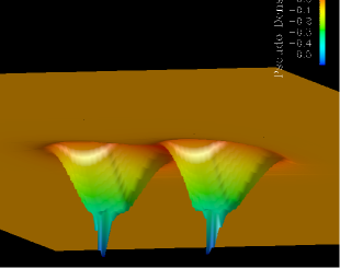
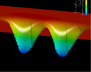
(a) Pseudo-density    (b) Coulomb potential

Figure 5: The pseudo-density and Coulomb potential for a palladium dimer on the $z=0$ plane

To solve the Poisson equation (3.2), we use a finite difference scheme and a multigrid method [12, 13, 14, 15], which is a well-known, rapid, and scalable solver of elliptic partial differential equations.

Then, we solve the spherical Poisson equation

$$\left(\frac{\partial^{2}}{\partial r^{2}}+\frac{2}{r}\frac{\partial}{\partial r}-\frac{L(L+1)}{r^{2}}\right)V_{LM}^{C}(r_{i})=4\pi\left(\rho_{LM}(r_{i})-\delta_{L0}Z_{i}\right),$$ (3.4)

inside a sphere with Dirichlet boundary conditions which come from the solution of (3.2), i.e.,

$$V_{\mbox{\scriptsize C}}(\mathbb{x})=\sum_{LM}V_{LM}^{C}(r_{i})y_{LM}(\hat{r}_{i})$$ (3.5)

where

$$V_{LM}^{C}(r_{i}) =V_{LM}^{C}(R_{i})\left(\frac{r_{i}}{R_{i}}\right)^{L}+\frac{4\pi}{2L+1}\left(\frac{1}{r_{i}^{L+1}}\int_{0}^{r_{i}}\rho_{LM}(r^{\prime})^{L+2}dr^{\prime}\right.$$

$$-\frac{Z_{i}}{\sqrt{4\pi}} \left(\frac{1}{r_{i}}-\frac{1}{R_{i}}\right)\delta_{L0}\left.-\frac{r_{i}^{L}}{R_{i}^{2L+1}}\int_{0}^{R_{i}}\rho_{LM}(r^{\prime})^{L+2}dr^{\prime}+r_{i}^{L}\int_{r_{i}}^{R_{i}}\rho_{LM}(r^{\prime})^{L-l}dr^{\prime}\right)$$

and

$$V_{LM}^{C}(R_{i}) =\int_{\partial S_{i}}V_{\mbox{\scriptsize C}}(\mathbb{x})y_{LM}(\mathbb{x})dS$$ (3.6)

$$\rho_{LM}(R_{i}) =\int_{\partial S_{i}}\rho(\mathbb{x})y_{LM}(\mathbb{x})dS.$$ (3.7)

Next, we consider the generation of the overlap matrix $S$ and the Hamiltonian matrix $H$ in the interstitial region and the spheres. From (2.1) we obtain

$$\int_{\Omega}\varphi_{i}(\mathbb{x})\left\{-\frac{1}{2}\nabla^{2}+V(\mathbb{x})\right\}\varphi_{k}(\mathbb{x})d\mathbb{x}=\int_{\Omega}\varphi_{i}(\mathbb{x})\varphi_{k}(\mathbb{x})d\mathbb{x}.$$ (3.8)

Using Green’s theorem the left-hand side (the Hamiltonian matrix) of (3.8) can be rewritten

$$\begin{split}\int_{\Omega}\varphi_{i}(\mathbb{x})&\left\{-\frac{1}{2}\nabla^{2}+V(\mathbb{x})\right\}\varphi_{k}(\mathbb{x})d\mathbb{x}\\ &=\int_{\Omega}\left(\frac{1}{2}\nabla\varphi_{i}(\mathbb{x})\nabla\varphi_{k}(\mathbb{x})+\varphi_{i}(\mathbb{x})V(\mathbb{x})\varphi_{k}(\mathbb{x})\right)d\mathbb{x}-\frac{1}{2}\int_{\partial\Omega}\nabla\varphi_{i}\frac{\partial\varphi_{k}}{\partial\mathbb{n}}d\mathbb{x}\end{split}$$

Thus, the Hamiltonian matrix is symmetric with zero Dirichlet or Neumann boundary conditions, but not in general. Thus we consider the following symmetric form derived from Green’s theorem and zero Dirichlet or Neumann boundary condition,

$$\int_{\Omega}\left(\frac{1}{2}\nabla\varphi_{i}(\mathbb{x})\nabla\varphi_{k}(\mathbb{x})+\varphi_{i}(\mathbb{x})V(\mathbb{x})\varphi_{k}(\mathbb{x})\right)d\mathbb{x}=\int_{\Omega}\varphi_{i}(\mathbb{x})\varphi_{k}(\mathbb{x})d\mathbb{x}.$$ (3.9)

The evaluation of (3.9) requires considerable computational effort, so we use the following symmetrized form

$$\begin{split}\frac{1}{2}\int_{\Omega}&\varphi_{i}(\mathbb{x})\left\{-\frac{1}{2}\nabla^{2}\right\}\varphi_{k}(\mathbb{x})+\varphi_{k}(\mathbb{x})\left\{-\frac{1}{2}\nabla^{2}\right\}\varphi_{i}(\mathbb{x})d\mathbb{x}\\ &+\int_{\Omega}\varphi_{i}(\mathbb{x})V(\mathbb{x})\varphi_{k}(\mathbb{x})d\mathbb{x}=\int_{\Omega}\varphi_{i}(\mathbb{x})\varphi_{k}(\mathbb{x})d\mathbb{x},\end{split}$$ (3.10)

In the interstitial region, we compute the contribution of the matrices $S^{*}$ and $H^{*}$ by

$$\begin{split}H_{inlm,i^{\prime}n^{\prime}l^{\prime}m^{\prime}}&=\frac{1}{2}\int_{\Omega-\cup_{i}S_{i}}\phi_{inlm}(\mathbb{x})\left\{-\frac{1}{2}\nabla^{2}+V(\mathbb{x})\right\}\phi_{i^{\prime}n^{\prime}l^{\prime}m^{\prime}}(\mathbb{x})\\ &+\phi_{i^{\prime}n^{\prime}l^{\prime}m^{\prime}}(\mathbb{x})\left\{-\frac{1}{2}\nabla^{2}+V(\mathbb{x})\right\}\phi_{inlm}(\mathbb{x})d\mathbb{x}\end{split}$$ (3.11)

$$S_{inlm,i^{\prime}n^{\prime}l^{\prime}m^{\prime}} =\int_{\Omega-\cup_{i}S_{i}}\phi_{inlm}(\mathbb{x})\phi_{i^{\prime}n^{\prime}l^{\prime}m^{\prime}}(\mathbb{x})d\mathbb{x},$$ (3.12)

where

$$\phi_{inlm}(\mathbb{x})=r_{i}^{n-1}\exp(-\zeta r_{i})y_{lm}(\hat{r}_{i}).$$ (3.13)

To compute the contribution of the matrices $S^{*}$ and $H^{*}$, we use the grid or mid-point of each cube, i.e.,

$$S^{1}_{inlm,i^{\prime}n^{\prime}l^{\prime}m^{\prime}}=\sum_{P}\phi_{inlm}(P)\phi_{i^{\prime}n^{\prime}l^{\prime}m^{\prime}}(C_{P})\mbox{Vol}(C_{P}),$$

or

$$S^{2}_{inlm,i^{\prime}n^{\prime}l^{\prime}m^{\prime}} =\sum_{C}\int_{C}\phi_{inlm}(\mathbb{x})\phi_{i^{\prime}n^{\prime}l^{\prime}m^{\prime}}(\mathbb{x})d\mathbb{x}$$

$$=\sum_{C}\phi_{inlm}(C)\phi_{i^{\prime}n^{\prime}l^{\prime}m^{\prime}}(C)\mbox{Vol}(C_{C}),$$

where $P$’s are the points of a uniform grid, $C$’s are the center of cube in uniform grid, and $\mbox{Vol}(C_{P})$ is the volume of a cube centered $P$. In each case, we have to compute $\phi_{ilmn}$ on all grid points for each $i,n,l,m$.

For the spherical coordinate operator

$$\nabla^{2}=\frac{\partial^{2}}{\partial r^{2}}+\frac{2}{r}\frac{\partial}{\partial r}+\frac{1}{r^{2}}\left[\frac{1}{\sin^{2}\phi}\frac{\partial^{2}}{\partial\theta^{2}}+\frac{\cos\phi}{\sin\phi}\frac{\partial}{\partial\phi}+\frac{\partial^{2}}{\partial\phi^{2}}\right]$$

and

$$\left[\frac{1}{\sin^{2}\phi}\frac{\partial^{2}}{\partial\theta^{2}}+\frac{\cos\phi}{\sin\phi}\frac{\partial}{\partial\phi}+\frac{\partial^{2}}{\partial\phi^{2}}+l(l+1)\right]y_{lm}=0,$$

we have

$$\begin{split}\ &\left[-\frac{1}{2}\nabla^{2}+V(\mathbb{x})\right]\phi_{inlm}(\mathbb{x})\\ &=\frac{1}{2}\left[(l(l+1)-n(n-1))r_{i}^{n-3}+2\zeta nr_{i}^{n-2}-\zeta^{2}r_{i}^{n-1}\right]\exp(-\zeta r_{i})y_{lm}(\hat{r}_{i})\\ &+V(\mathbb{x})r_{i}^{n-1}\exp(-\zeta r_{i})y_{lm}(\hat{r}_{i})=\tilde{\phi}_{inlm}(\mathbb{x}).\end{split}$$ (3.14)

So, we have to compute

$$H^{1}_{inlm,i^{\prime}n^{\prime}l^{\prime}m^{\prime}} =\frac{1}{2}\sum_{P}\left(\phi_{inlm}(P)\tilde{\phi}_{i^{\prime}n^{\prime}l^{\prime}m^{\prime}}(P)+\phi_{i^{\prime}n^{\prime}l^{\prime}m^{\prime}}(P)\tilde{\phi}_{inlm}(P)\right)\mbox{Vol}(P),$$

$$S^{1}_{inlm,i^{\prime}n^{\prime}l^{\prime}m^{\prime}} =\sum_{P}\phi_{inlm}(P)\phi_{i^{\prime}n^{\prime}l^{\prime}m^{\prime}}(P)\mbox{Vol}(P),$$

i.e., $\phi_{inlm}(P)$ and $\tilde{\phi}_{inlm}(P)$ at each regular cubic grid point which does not include any spheres.

For the contribution of $S$ and $H$ inside spheres, we can compute the elements of the matrices with given $\beta$’s and $\alpha$’s as in [1].

$$S_{inlm,i^{\prime}l^{\prime}m^{\prime}n^{\prime}}^{j} =\int_{S_{j}}\phi_{inlm}(\mathbb{x})\phi_{i^{\prime}l^{\prime}m^{\prime}n^{\prime}}(\mathbb{x})d\mathbb{x}$$

$$=\sum_{j\lambda\mu}(\beta_{inlm,j\lambda\mu}\beta_{i^{\prime}n^{\prime}l^{\prime}m^{\prime},j\lambda\mu}+\alpha_{inlm,j\lambda\mu}\alpha_{i^{\prime}n^{\prime}l^{\prime}m^{\prime},j\lambda\mu}<\dot{g}_{j\lambda}|\dot{g}_{j\lambda}>),$$

$$H_{inlm,i^{\prime}l^{\prime}m^{\prime}n^{\prime}}^{j} =\frac{1}{2}\int_{S_{j}}\left(\phi_{inlm}(\mathbb{x})\left\{-\frac{1}{2}\nabla^{2}+V(\mathbb{x})\right\}\phi_{i^{\prime}l^{\prime}m^{\prime}n^{\prime}}(\mathbb{x})\right.$$

$$\left.\phi_{i^{\prime}n^{\prime}l^{\prime}m^{\prime}}(\mathbb{x})\left\{-\frac{1}{2}\nabla^{2}+V(\mathbb{x})\right\}\phi_{ilmn}(\mathbb{x})\right)d\mathbb{x}$$

$$=e_{j}S_{inlm,i^{\prime}l^{\prime}m^{\prime}n^{\prime}}^{j}+\frac{1}{2}\sum_{j\lambda\mu}\left(\beta_{inlm,j\lambda\mu}\alpha_{i^{\prime}n^{\prime}l^{\prime}m^{\prime},j\lambda\mu}+\alpha_{inlm,j\lambda\mu}\beta_{i^{\prime}n^{\prime}l^{\prime}m^{\prime},j\lambda\mu}\right)$$

$$+\sum_{\lambda\mu,\lambda^{\prime}\mu^{\prime},LM,L>0}\int_{0}^{R_{j}}[\beta_{inlm,j\lambda\mu}g_{j\lambda}(r)+\alpha_{inlm,j\lambda\mu}\dot{g}_{j\lambda}(r)]V_{LM}(r)$$

$$\cdot[\beta_{i^{\prime}n^{\prime}l^{\prime}m^{\prime},j\lambda^{\prime}\mu^{\prime}}g_{j\lambda^{\prime}}(r)+\alpha_{i^{\prime}n^{\prime}l^{\prime}m^{\prime},j\lambda^{\prime}\mu^{\prime}}\dot{g}_{j\lambda^{\prime}}(r)]r^{2}drI_{R}(\lambda\mu,\lambda^{\prime}\mu^{\prime},LM),$$

where $I_{R}(\lambda\mu,\lambda^{\prime}\mu^{\prime},LM)$ is a real Gaunt Integral.

To solve the eigenvalue problems $H\varphi_{k}=\epsilon_{k}S\varphi_{k}$ where $H$ and $S$ are real symmetric and dense matrices and $S$ is positive definite with dimension $n=N_{\mbox{\scriptsize basis}}$, we use ScaLAPACK [16], which is well developed and optimized for parallel machines.

Here, we consider updating the charge density from the solutions of $H\varphi_{k}=\epsilon_{k}S\varphi_{k}$.

We have to compute $\rho_{\mbox{\scriptsize out}}=\sum_{\epsilon_{k}<E_{\mbox{\scriptsize Fermi}}}|\varphi_{k}|^{2}+\rho_{\mbox{\scriptsize core}}$ in the whole region including both the spheres and the interstitial region. We write $\varphi_{k}$

$$\varphi_{k}=\sum_{inlm}\varphi_{k,inlm}\phi_{inlm}.$$

In the interstitial region, we compute

$$\rho_{\mbox{\scriptsize out}}(\mathbb{x})=\sum_{\epsilon_{k}<E_{\mbox{\scriptsize Fermi}}}|\varphi_{k}(\mathbb{x})|^{2},$$

where

$$\varphi_{k}(\mathbb{x})=\sum_{inlm}\varphi_{k,inlm}(r_{i}^{n-1}e^{-\zeta r_{i}}y_{lm}(\hat{r}_{i}))$$

at all regular cubic grid points $\mathbb{x}$.

Inside the spheres, we compute

$$\rho(\mathbb{x})=\sum_{jLM}\rho_{jLM}y_{LM}(\hat{r}_{j})+\rho_{\mbox{\scriptsize core}}=\sum_{\epsilon_{k}<E_{\mbox{\scriptsize Fermi}}}|\varphi_{k}(\mathbb{x})|^{2}+\rho_{\mbox{\scriptsize core}}.$$ (3.15)

From the orthogonality of $g$ and $\dot{g}$, we have

$$\rho_{jLM} =\int_{\partial S_{j}(r_{j})}\varphi_{k}^{2}y_{LM}(\hat{r}_{j})ds$$

$$=\sum_{inlm}\sum_{i^{\prime}n^{\prime}l^{\prime}m^{\prime}}\sum_{j\lambda\mu}\sum_{j\lambda^{\prime}\mu^{\prime}}\varphi_{k,inlm}\varphi_{k,i^{\prime}n^{\prime}l^{\prime}m^{\prime}}[\beta_{inlm,j\lambda\mu}g_{j\lambda}(r_{j})+\alpha_{inlm,j\lambda\mu}\dot{g}_{j\lambda\mu}(r_{j})]$$

$$[\beta_{i^{\prime}n^{\prime}l^{\prime}m^{\prime},j\lambda^{\prime}\mu^{\prime}}g_{j\lambda^{\prime}}(r_{j})+\alpha_{i^{\prime}n^{\prime}l^{\prime}m^{\prime},j\lambda^{\prime}\mu^{\prime}}\dot{g}_{j\lambda^{\prime}\mu^{\prime}}(r_{j})]I_{R}(LM,\lambda\mu,\lambda^{\prime}\mu^{\prime}).$$

4 Results

To test the method we have calculated the total energy for several palladium clusters.

The total energy is computed in the usual way

$$E =-\sum_{k}^{\mbox{occ}}\int_{\Omega}\varphi_{k}(\mathbb{x})\frac{\nabla^{2}}{2}\varphi_{k}(\mathbb{x})d\mathbb{x}+\int_{\Omega}V_{\mbox{\scriptsize Ext}}(\mathbb{x})\rho(\mathbb{x})d\mathbb{x}$$

$$+\frac{1}{2}\int_{\Omega}\int_{\Omega}\frac{\rho(\mathbb{x})\rho(\mathbb{x}^{\prime})}{|\mathbb{x}-\mathbb{x}^{\prime}|}d\mathbb{x}^{\prime}d\mathbb{x}+E_{\mbox{\scriptsize xc}},$$

where the terms are respectively the non-interacting kinetic energy, the external potential, the Hartree and the exchange and correlation energies. This formula can be simplified using (2.1) to yield

$$E=\sum_{k}^{\mbox{occ}}\epsilon_{k}-\frac{1}{2}\int_{\Omega}V_{\mbox{\scriptsize Hartree}}(\mathbb{x})\rho(\mathbb{x})d\mathbb{x}-\int_{\Omega}V_{\mbox{\scriptsize xc}}(\mathbb{x})\rho(\mathbb{x})d\mathbb{x}+E_{\mbox{\scriptsize xc}},$$ (4.1)

where

$$E_{\mbox{\scriptsize xc}}=\int_{\Omega}e_{\mbox{\scriptsize xc}}(\mathbb{x})\rho(\mathbb{x})d\mathbb{x}.$$

There have been many calculations of the energetics of Pd clusters in recent years [18, 19, 20, 21, 22]. Most calculations show that small clusters are magnetic (spin polarized) and for example that $Pd_{13}$ has an icosohedral or possibly a buckled biplanar structure [19]. Since our purpose is to test the method, we have compared results for non-magnetic structures in simpler geometries.

The LASTO basis set was optimized for crystalline palladium in the facecentered cubic structure. It consistes of two $s$, two $p$, and two $d$ functions plus one $f$ function per atom. The $\zeta$ values are given in Table 1.

Table 1: LASTO Basis and $\zeta$ values

function	$\zeta(a_{0}^{-1})$
4d	2.20
5d	2.60
5s	1.00
5p	1.00
6s	2.00
6p	2.00
4f	1.60

The 1s through 4p states were treated as core functions. They are solved using the full Dirac equation in the spherical part of the potential within the spheres. A logarithmic radial mesh was used inside the spheres, with 429 points. The (uniform) mesh in the interstitial region had a spacing of $0.05$ $a_{0}$. Calculations with NWchem used the SBKJC basis with an effective core potential given in [17]. In both sets of calculations states near the highest occupied level were smeared with a Gaussian of $\approx 0.001au$.

In Fig. 6 we plot the binding energy of a palladium dimer as a function of $r$ with LSD and GGA expressions for exchange and correlation energy. Here we computed the binding energy per atom by

$$E=\frac{E(Pd_{n})-nE(Pd)}{n}$$

and fitted the data with Morse potential energy function, i.e.,

$$E(r)=D\left\{e^{-2a(r-R_{0})}-2e^{-a(r-R_{0})}\right\}$$

where D is the minimum energy, $R_{0}$ is the equilibrium internuclear distance.

Figure 6: Binding energy of Pd₂ in units of Hatrees/atom as a function of the separation distance $r$ in atomic units. The smooth curves are fits to a Morse potential.

In Table 2, we compare the results with experiment [23][24][25] and with numerical results of Zhang, Ge, and Wang [20], which use plane wave basis sets and GGA for exchange and correlation energy, and DMol³ [27] program which uses LCAO (Linear combination of atomic orbital) with several methods for the exchange and correlation energy. Our results for both the internuclear distance and the binding energy are in agreement with previous calculations.

Table 2: Binding energy for a Palladium (Pd) dimer with comparing previous results

	binding energy	$R_{0}$
Experiment [23]	$0.37\pm 0.13$ eV/atom	4.71 au
Experiment [24]	$0.52\pm 0.08$ eV/atom	4.71 au
Experiment [25]	0.698 eV/atom	4.71 au
LASTO(PBE-GGA)	0.559 eV/atom	4.802 au
LASTO(LSD)	0.882 eV/atom	4.604 au
Plane wave, GGA [20]	0.63 eV/atom	4.70 au
DMol3(PBE-GGA – LCAO)[27]	0.415 eV/atom	4.70 au
DMol3(PW91-GGA – LCAO) [27]	0.538 eV/atom	4.70 au
DMol3(PW-LSD – LCAO)[27]	0.770 eV/atom	4.70 au
NWChem (PBE-GGA)[26]	0.468 eV/atom	4.802 au

In Fig. 7, we present the structures of Pd₂, Pd₄, and Pd₈. We calculate the binding energy for Pd₂, for Pd₄, and for Pd₈ with LSD and GGA methods for the exchange and correlation energy. The bond lengths were chosen to be the same as [20] and were not varied. In Table 3, we present the results and compare with the results of [20] and with [28]. Again the energies show agreement with previous work.

Figure 7: Structures of dimer and 4- and 8- Pd clusters used to test the LASTO code

Table 3: Binding energy in $eV/atom$ for Pd₂, Pd₄, and Pd₈

	Pd2	Pd4	Pd8
LASTO (LSD)	0.861	1.633	2.700
LASTO (PBE-GGA)	0.559	1.265	2.189
Plane wave (GGA)	.473	1.234	1.995
Plane wave (GGA) [20]	0.63	1.46	1.91
NWChem (PBE-GGA)	0.468	1.405	1.869

5 Conclusion

In summary we have shown that a real space version of the linear augmented Slater type orbital method provides good agreement with other calculations for small clusters. The full treatment of core orbitals while maintaining a small basis set will be useful for treating heavy elements such as Pt or Au which are important nanoscale systems.

References

• [1] Davenport, J.W. , Physical Review B, 1984, 29, 2898.
• [2] Davenport, J.W., Weinert, M. and Watson, R.E., Physical Review B, 1985, 32, 4876.
• [3] Fernando, G.W., Davenport, J.W., Watson, R.E. and Weinert, M., Physical Review B, 1989, 40, 2757.
• [4] Anderson,O.K., Phys. Rev. B 1975, 12 3060.
• [5] Beck, T.L., Rev. Mod. Phys. 2000, 72,1041.
• [6] Chelikowski, J.R., Troullier, N., Saad,Y., Phys. Rev. Lett. 1994, 72, 1240.
• [7] Li, S., Alemany, M.M.G., Chelikowski, J.R., J. Chem. Phys. 2006, 125, 034311.
• [8] Weinert, M., J. Math. Phys. 1981, 22, 2433.
• [9] Mattheiss, L.F., Hamann, D.R., Phys. Rev. B 1986, 33, 823.
• [10] Martin, R.M. “ Electronic Structure Basic Theory and practical methods”, Cambridge University Press, 2004.
• [11] Perdew, J.P., Burke, K. and Wang, Y., Physical Review B 1996, 54, 16533, Perdew, J.P., Burke, K. and Ernzerhof, Phys. Rev. Lett. 1996, 77, 3875.
• [12] Bramble, J., “Multigrid Methods”, Pitman, London, 1993.
• [13] Brandt, A., “Multigrid Techniques: 1984 Guide, with Applications to Fluid Dynamics”, GMD studien 85, GMD, Forschungszentrum Informationstechnik, St. Augustin, Germany, 1984.
• [14] Hackbush, W., “ Multigrid Methods and Applications”, Springer-Verlag, Berlin, 1985.
• [15] Wesseling, P., “An Introduction to Multigrid Methods”, John Wiely, Chichester, UK, 1992.
• [16] www.netlib.org/scalapack/.
• [17] Stevens, W.J., Krauss, M., Basch, H., Jasien, P.G., Can. J. Chem., 1992, 70, 612.
• [18] Moseler, M., Hakkinen, H., Barnett, R.N¿, Landman, U., Phys. Rev. Lett. 2001, 86, 2545.
• [19] Kumar, V., Kawazoe, Y., Phys. Rev. B 2002, 66, 144413.
• [20] Zhang, W., Ge, Q. and Wang, L., Journal of Chemical Physics 2003, 118, 5793.
• [21] Chang, C.M., Chou, M.Y., Phys. Rev. Lett. 2004, 93, 133401.
• [22] Longo, R.C., Gallego, L.J., Phys. Rev. B 2006, 74, 193409.
• [23] Lin, S-S, Strauss, B., and Kant, A., J. Chem. Phys. 1969, 51, 2282.
• [24] Shim, I., and Gingerich, K.A., J. Chem. Phys. 1984, 80, 5107.
• [25] Huber, K.P. and Herzberg, G., “Molecular Spectra and Molecular Structure, 4: Constants of Diatomic Molecules”, Van Nostrand Reinhold, New York, 1979.
• [26] ”High Performance Computational Chemistry: An Overview of NWChem a Distributed Parallel Application,” Kendall, R.A.; Apra, E.; Bernholdt, D.E.; Bylaska, E.J.; Dupuis, M.; Fann, G.I.; Harrison, R.J.; Ju, J.; Nichols, J.A.; Nieplocha, J.; Straatsma, T.P.; Windus, T.L.; Wong, A.T.; Computer Phys. Comm. 2000, 128, 260.
• [27] “http://www.accelrys.com/products/mstudio/modeling/quantumandcatalysis/dmol3.html” We thank S. Chaudhuri for kindly providing these numbers.
• [28] Futschek, T., Marshmen, M., Hafner, J., J. Phys. Cond. Matt. 2005, 17, 5927.