Relaxation of a Single Knotted Ring Polymer

Abstract

The relaxation of a single knotted ring polymer is studied by Brownian dynamics simulations. The relaxation rate $\lambda_{q}$ for the wave number $q$ is estimated by the least square fit of the equilibrium time-displaced correlation function $\hat{C}_{q}(t)=N^{-1}\sum_{i}\sum_{j}\frac{1}{3}\langle\mib{R}_{i}(t)\cdot\mib{R}_{j}(0)\rangle\exp[{\rm i}{2\pi}q(j-i)/N]$ to a double exponential decay at long times. Here, $N$ is the number of segments of a ring polymer and $\mib{R}_{i}$ denotes the position of the $i$th segment relative to the center of mass of the polymer. The relaxation rate distribution of a single ring polymer with the trivial knot appears to behave as $\lambda_{q}\simeq A(1/N)^{x}$ for $q=1$ and $\lambda_{q}\simeq A^{\prime}(q/N)^{x^{\prime}}$ for $q>1$, where $x\simeq 2.10$, $x^{\prime}\simeq 2.17$ and $A<A^{\prime}$. These exponents are similar to that found for a linear polymer chain. The topological effect appears as the separation of the power law dependences for $q=1$ and $q>1$, which does not appear for a linear polymer chain. In the case of the trefoil knot, the relaxation rate distribution appears to behave as $\lambda_{q}\simeq A(1/N)^{x}$ for $q=1$ and $\lambda_{q}\simeq A^{\prime}(q/N)^{x^{\prime}}$ for $q=2$ and $3$, where $x\simeq 2.61$, $x^{\prime}\simeq 2.02$ and $A>A^{\prime}$. The wave number $q$ of the slowest relaxation rate $\lambda_{q}$ for each $N$ is given by $q=2$ for small values of $N$, while it is given by $q=1$ for large values of $N$. This crossover corresponds to the change of the structure of the ring polymer caused by the localization of the knotted part to a part of the ring polymer.

1 Introduction

The effects of topological constraints caused by the entanglement of polymers on the properties of polymer systems have attracted much attention.[1, 2, 3, 4, 5, 6, 7, 8, 9, 10, 11, 12, 13, 16, 17, 18, 19, 20, 21, 14, 15] One of the famous theories on the topological effects is the reptation theory[1, 2] of the dynamics of concentrated polymer systems, where polymers are entangled each other. In this theory, the topological constraints on a polymer chain caused by the surrounding polymer chains are replaced by an effective tube confining the polymer chain. The predictions of the theory with corrections due to the finiteness of polymer length[2] agree with the experimental results and have been confirmed by simulations.[3, 4] In concentrated polymer systems, the entanglement of polymers changes dynamically and the topological constraints change accordingly. In contrast, in the case of a single knotted ring polymer, which is one of the self-entangled systems, the topological constraints are determined by the knot type and do not change with time. Therefore, a single ring polymer system can be considered as an ideal system for the study of topological effects. The investigation of the effects of knots in this system is expected to provide a basis for further understanding of the topological effects in polymer systems.

The interest in the properties of knotted ring polymers has been growing in recent years.[5, 6, 7, 8, 9, 10, 11, 12, 13, 16, 17, 18, 19, 20, 21, 14, 15] Especially, the topological effects on the static properties of ring polymers have been well studied.[6, 7, 8, 9, 10, 11, 12, 13, 14, 15] It was conjectured by des Cloizeaux that topological constraints make ring polymers with long chains swell.[6] Although this swelling effect caused by effective repulsion among segments is supported by a computer simulation[7] and a scaling analysis,[8] there have been studies[9, 10, 11, 12, 13] predicting that the effect vanishes in the long chain limit. In contrast to the static properties, the topological effects on the dynamics are less well studied.[16, 17, 18] The equilibrium relaxation of single knotted ring polymers has been studied by measuring the time autocorrelation function of the radius of gyration of a knotted ring polymer and the long relaxation time that does not appear for the trivial knot has been found.[16] The relaxation time has the dependence on the number of the essential crossings $C$.[17] The nonequilibrium relaxation after cutting one bond of a knotted ring polymer has been studied and the distribution of the nonequilibrium relaxation time of the radius of gyration has been found to show different behavior for different knot groups.[5, 18] Experimentally, knotted circular DNA molecules have been studied by using gel electrophoresis, electron microscopy, and so on.[19, 20, 21]

In the case of linear polymers, the relaxation phenomena have been studied systematically in terms of the relaxation modes and rates.[22, 23, 24, 25, 26, 27, 3] The relaxation modes and rates are given as left eigenfunctions and eigenvalues of the time-evolution operator of the master equation of the system, respectively.[22, 23, 24] The equilibrium time correlation functions of the relaxation modes satisfy $\langle X_{p}(t)X_{q}(0)\rangle\propto\delta_{p,q}\exp(-\lambda_{p}t),$ where $X_{p}$ and $\lambda_{p}$ denote the $p$th relaxation mode and its relaxation rate, respectively. For single linear polymers represented by the Rouse model, which has no excluded volume interaction and no hydrodynamic interaction, the relaxation modes are identical to the Rouse modes, which have been playing an important role in the theory of the polymer dynamics.[28, 29, 2] For single linear polymers with the excluded volume interaction and without the hydrodynamic interaction, the relaxation modes and rates are estimated by solving a generalized eigenvalue problem $\sum_{j=1}^{N}C_{i,j}(t_{0}+\tau)f_{p,j}=\exp(-\lambda_{p}\tau)\sum_{j=1}^{N}C_{i,j}(t_{0})f_{p,j}$ under the orthonormal condition $\sum_{i=1}^{N}\sum_{j=1}^{N}f_{p,i}C_{i,j}(t_{0})f_{q,j}=\delta_{p,q}$,[23, 24] where $C_{i,j}(t)$ denotes the equilibrium time-displaced correlation function $\frac{1}{3}\langle\mib{R}_{i}(t)\cdot\mib{R}_{j}(0)\rangle$ of the position of the $i$th segment relative to the center of mass of the polymer $\mib{R}_{i}$ and that of the $j$th segment and $N$ denotes the number of the segments of the polymer. The $p$th relaxation mode and the corresponding relaxation rate are given by $f_{p,i}$ and $\lambda_{p}$, respectively. The behavior of the contribution $g_{i,p}$ of the $p$th slowest relaxation mode to $\mib{R}_{i}$ is similar to that of the Rouse mode, $g_{i,p}\propto\cos\left[\pi p(i-\frac{1}{2})/N\right]$, and the corresponding relaxation rate $\lambda_{p}$ behaves as $\lambda_{p}\propto(p/N)^{2\nu+1}$.[2, 23, 24] Here, $\nu\simeq 0.588$ is the exponent for the power law dependence of the size of a single linear polymer with the excluded volume interaction on the number of the segments of the polymer.

The purpose of the present paper is to examine the effects of the topological constraints on the relaxation of single ring polymers by carrying out an analysis similar to that which has been done for linear single polymers. Brownian dynamics simulations of single ring polymers with the trivial knot and the trefoil knot are performed, where the excluded volume interaction is taken into account and the hydrodynamic interaction is neglected, and the distribution of relaxation rates is estimated.

In §2, a model used in the present paper and the method for the estimation of the relaxation rates are explained. The results of the simulations are presented in §3. Summary and discussion are given in the last section.

2 Model and Relaxation Rates

In order to study a single knotted ring polymer in good solvent, Brownian dynamics simulations of a bead-spring model are performed. The dynamics of the $i$th segment of a single ring polymer with $N$ segments is described by the Langevin equation

$$\frac{{\rm d}\mib{r}_{i}(t)}{{\rm d}t}=-\frac{1}{\zeta}\frac{{\partial}V(\{\mib{r}_{j}\})}{{\partial}\mib{r}_{i}}+\mib{w}_{i}(t).$$ (1)

Here, $\mib{r}_{i}(t)$ denotes the position of the $i$th segment at time $t$ and $\zeta$ is the friction constant. The random force $\zeta\mib{w}_{i}(t)$ acting on the $i$th segment is a Gaussian white stochastic process satisfying $\langle w_{i,\alpha}(t)\rangle=0$ and

$$\langle w_{i,\alpha}(t)w_{j,\beta}(t^{\prime})\rangle=2\frac{k_{{\rm B}}T}{\zeta}\delta_{i,j}\delta_{\alpha,\beta}\delta(t-t^{\prime}),$$ (2)

where $w_{i,\alpha},k_{{\rm B}}$ and $T$ denote the $\alpha$-component of $\mib{w}_{i}$, the Boltzmann constant and the temperature of the system, respectively. The potential $V(\{\mib{r}_{j}\})=V(\mib{r}_{1},\cdots,\mib{r}_{N})$ describes the interaction between the segments. In eq. (1), the hydrodynamics interaction is neglected.

In the present paper, we use the potential given by[30, 31, 32, 24]

$$V(\{\mib{r}_{j}\})=\sum_{i=2}^{N}\sum_{j=1}^{i-1}V_{{\rm R}}(|\mib{r}_{i}-\mib{r}_{j}|)+\sum_{i=1}^{N}V_{{\rm A}}(|\mib{r}_{i+1}-\mib{r}_{i}|)$$ (3)

with

$$V_{{\rm R}}(r)=\left\{\begin{array}[]{lll}\displaystyle 4\epsilon\Bigl{[}\Bigl{(}\frac{\sigma}{r}\Bigr{)}^{12}-\Bigl{(}\frac{\sigma}{r}\Bigr{)}^{6}+\frac{1}{4}\Bigr{]}&{\rm for}&r\leq 2^{\frac{1}{6}}\sigma,\\ 0&{\rm for}&r>2^{\frac{1}{6}}\sigma,\end{array}\right.$$ (4)

and

$$V_{{\rm A}}(r)=\left\{\begin{array}[]{lll}\displaystyle-\frac{1}{2}kR_{0}^{2}\ln\Bigl{[}1-\Bigl{(}\frac{r}{R_{0}}\Bigr{)}^{2}\Bigr{]}&{\rm for}&r\leq R_{0},\\ \infty&{\rm for}&r>R_{0}.\end{array}\right.$$ (5)

Here, $V_{{\rm R}}$ is the repulsive part of the Lennard-Jones potential and represents the excluded volume interaction between all the segments. The potential $V_{{\rm A}}$ is called a finitely extensible nonlinear elastic (FENE) potential and represents the attractive interaction between neighboring segments along the ring polymer.[32] In the last summation of the right hand side of eq. (3), $\mib{r}_{N+1}=\mib{r}_{1}$ because the $N$th segment is connected to the first segment along the ring polymer.

As mentioned in the previous section, the relaxation modes and rates are given as left eigenfunctions and eigenvalues of the time-evolution operator of the master equation of the system, respectively.[22, 23, 24] In the previous studies on the relaxation modes and rates of single linear polymers, a trial function for the $p$th relaxation mode is chosen to be $\mib{X}_{p}(Q)=\sum_{i=1}^{N}f_{p,i}\mib{R}_{i}(t_{0}/2;Q)$, where $Q$ represents a state of the system and $\mib{R}_{i}(t_{0}/2;Q)$ denotes the expectation value of $\mib{R}_{i}$ after a period $t_{0}/2$ starting from a state $Q$. The quantity $\mib{R}_{i}$ denotes the position of the $i$th segment relative to the center of mass of the polymer: $\mib{R}_{i}=\mib{r}_{i}-\mib{r}_{\rm c}$ with $\mib{r}_{c}=\frac{1}{N}\sum_{i=1}^{N}\mib{r}_{i}$. For this trial function, a variational problem equivalent to the eigenvalue problem for the time-evolution operator leads to a generalized eigenvalue problem $\sum_{j=1}^{N}C_{i,j}(t_{0}+\tau)f_{p,j}=\exp(-\lambda_{p}\tau)\sum_{j=1}^{N}C_{i,j}(t_{0})f_{p,j}$ mentioned in the previous section, where $C_{i,j}(t)=\frac{1}{3}\langle\mib{R}_{i}(t)\cdot\mib{R}_{j}(0)\rangle$ is the equilibrium time-displaced correlation function. This analysis is considered to extract the slow relaxation modes contained in the quantities $\{\mib{R}_{i}\}$ and to give better results as $t_{0}$ becomes larger, because the contribution of faster relaxation modes contained in $\mib{R}_{i}(t_{0}/2;Q)$ becomes smaller.

In the case of single ring polymers, the eigenfunctions $f_{p,j}$ of the above-mentioned generalized eigenvalue problem are known because of the translational invariance of the segment number along the ring polymer: $C_{i,j}(t)=C_{i+l,j+l}(t)$, where the subscripts representing the segment numbers are considered modulo $N$. The eigenfunctions are given by $f_{q,j}\propto\exp\left({\rm i}2\pi qj/N\right)$ with $q=1,\cdots,N-1$.[33] Note that the wave number $q=0$ is not included for it gives a meaningless relaxation mode $\sum_{j=1}^{N}\mib{R}_{j}(t_{0}/2;Q)=\mib{0}$ with an eigenvalue $\exp(-\lambda_{q}\tau)=0$, because $\sum_{j=1}^{N}\mib{R}_{j}=\mib{0}$ and $\sum_{j=1}^{N}C_{i,j}(t)=0$. For the eigenfunction with the wave number $q$, the generalized eigenvalue problem is reduced to

$$\hat{C}_{q}(t_{0}+\tau)=\exp(-\lambda_{q}\tau)\hat{C}_{q}(t_{0}),$$ (6)

where $\hat{C}_{q}(t)$ denotes the Fourier transform of the correlation matrix given by

$$\hat{C}_{q}(t) = \sum_{l=0}^{N-1}C_{i,i+l}(t)\exp\left({\rm i}\frac{2\pi}{N}ql\right)$$ (7)

$$= \sum_{l=0}^{N-1}C_{i,i+l}(t)\cos\left(\frac{2\pi}{N}ql\right).$$ (8)

Note that $C_{i,i+l}(t)$ does not depend on $i$ and is identical to $C_{i,i-l}(t)$. The equilibrium time-displaced correlation function of the Fourier transform $\hat{\mib{R}}_{q}$ of $\mib{R}_{i}$, which is defined by

$$\hat{\mib{R}}_{q}=\frac{1}{\sqrt{N}}\sum_{j=1}^{N}\mib{R}_{j}\exp\left({\rm i}\frac{2\pi}{N}qj\right),$$ (9)

is also given by $\hat{C}_{q}(t)$ as

$$\hat{C}_{q}(t)=\frac{1}{3}\langle\hat{\mib{R}}_{q}(t)\cdot\hat{\mib{R}}_{-q}(0)\rangle.$$ (10)

In the following, we only consider $\hat{C}_{q}(t)$ with $q=1,2,\cdots,\left\lfloor N/2\right\rfloor$, since $\hat{C}_{q}(t)=\hat{C}_{N-q}(t)$ as can be seen from eq. (8). Here, $\left\lfloor x\right\rfloor$ denotes the floor function of a real number $x$. Equation (6) is equivalent to the estimation of the relaxation rate $\lambda_{q}$ for the wave number $q$ from the values of $\hat{C}_{q}(t)$ at times $t_{0}$ and $t_{0}+\tau$ by assuming a single exponential decay of $\hat{C}_{q}(t)$ at these times. In fact, $\hat{C}_{q}(t)$, which is the autocorrelation function of the Fourier transform of $\mib{R}_{i}$, can be expressed as $\hat{C}_{q}(t)=a_{q}^{(1)}\exp(-\lambda_{q}^{(1)}t)+a_{q}^{(2)}\exp(-\lambda_{q}^{(2)}t)+\cdots$, where $0<\lambda_{q}^{(1)}<\lambda_{q}^{(2)}<\cdots$ and $a_{q}^{(k)}>0$ for $k=1,2,\cdots$.[22, 23] Thus, the estimation of the slowest relaxation rate $\lambda_{q}^{(1)}$ by eq. (6) becomes better as $t_{0}$ becomes larger, as mentioned before. In this paper, we estimate $\lambda_{q}^{(1)}$, the slowest relaxation rate in $\hat{C}_{q}(t)$ for the wave number $q$, by fitting several tens of values of $\hat{C}_{q}(t)$ at relatively long times estimated from the simulations to a double exponential decay form

$$\hat{C}_{q}(t)=a_{q}^{(1)}\exp(-\lambda_{q}^{(1)}t)+a_{q}^{(2)}\exp(-\lambda_{q}^{(2)}t),$$ (11)

because this method is more tolerant of statistical errors in the estimated values of $\hat{C}_{q}(t)$ than using eq. (6).

In the linearization approximation of Doi and Edwards,[2, 23] the relaxation rate $\lambda_{p}$ of the $p$th Rouse mode $\mib{X}_{p}=\left(2/N\right)^{1/2}\sum_{i=1}^{N}\mib{R}_{i}\cos\left[p\pi(i-\frac{1}{2})/N\right]$ of a single linear polymer with the excluded volume interaction is estimated from the static correlation $\langle\mib{X}_{p}\cdot\mib{X}_{p}\rangle$ as $\lambda_{p}^{({\rm LA})}=\left(k_{\rm B}T/\zeta\right)\left(\frac{1}{3}\langle\mib{X}_{p}\cdot\mib{X}_{p}\rangle\right)^{-1}$. In the case of single ring polymers, the relaxation rate $\lambda_{q}$ for the wave number $q$ is given by the linearization approximation as

$$\lambda_{q}^{{\rm(LA)}}=\frac{k_{{\rm B}}T}{\zeta}\left(\frac{1}{3}\langle\hat{\mib{R}}_{q}\cdot\hat{\mib{R}}_{-q}\rangle\right)^{-1}=\frac{k_{{\rm B}}T}{\zeta}\hat{C}_{q}(0)^{-1}.$$ (12)

These formulae are derived as follows.[2] In the linearization approximation, the equation of motion of each mode $x$ is approximated by the linear Langevin equation $\dot{x}=-\lambda x+w$, where the Gaussian white random force $w(t)$ satisfies $\langle w(t)\rangle=0$ and $\langle w(t)w(t^{\prime})\rangle=2D\delta(t-t^{\prime})$. On the basis of the relation $\langle x^{2}\rangle=D/\lambda$, which holds for this Langevin equation, the relaxation rate $\lambda$ is estimated from the mean square amplitude of the mode $\langle x^{2}\rangle$ as $\lambda=D/\langle x^{2}\rangle$. Thus, the relaxation rate given by the linearization approximation becomes small as the mean square amplitude of the mode vector, $\mib{X}_{p}$ or $\hat{\mib{R}}_{q}$, becomes large. The mode vector $\mib{X}_{p}$ for the linear polymer roughly corresponds to the end-to-end vector of a partial chain with a length of $N/p$ segments and $\hat{\mib{R}}_{q}$ for the ring polymer roughly corresponds to the end-to-end vector of a partial chain with a length of $N/(2q)$ segments. For a single linear polymer, the results of the linearization approximation are found to be consistent with those of the Monte Carlo simulations [23] and the molecular dynamics simulations. [24] In this paper, the relaxation rates $\lambda_{q}^{({\rm LA})}$ given by the linearization approximation for a single ring polymer are estimated by using eq. (12) and compared with the relaxation rates $\lambda_{q}^{(1)}$.

3 Results of Simulations

Brownian dynamics simulations of the model described in the previous section are performed for $N=24$, $36$, $48$, $72$, $96$, $144$ and $192$. The following parameters[24, 31] are used: $k_{{\rm B}}T/\epsilon=1$, $k\sigma^{2}/\epsilon=30$ and $R_{{\rm 0}}/\sigma=1.5$. The Euler algorithm with a time step ${\mit\Delta}t=1.4\times 10^{-4}\gamma\sigma^{2}/\epsilon$ is employed for a numerical integration of the equation of motion (1). Hereafter, we set $\sigma=1$, $\gamma=1$ and $\epsilon=1$.

The correlation function $\hat{C}_{q}(t)$ is calculated from $C_{i,j}(t)=\frac{1}{3}\langle\mib{R}_{i}(t)\cdot\mib{R}_{j}(0)\rangle$ estimated by the simulations by using Eq. (8). The equilibrium average $\langle\mib{R}_{i}(t)\cdot\mib{R}_{j}(0)\rangle$ is estimated as the time average over $M_{{\rm c}}$ configurations after the initial $M_{{\rm i}}$ configurations, which are discarded for the equilibration:

$$\langle\mib{R}_{i}(t)\cdot\mib{R}_{j}(0)\rangle=\frac{1}{M_{{\rm c}}}\sum_{n=M_{{\rm i}}+1}^{M_{{\rm i}}+M_{{\rm c}}}\mib{R}_{i}(n{\mit\Delta}T)\cdot\mib{R}_{j}(n{\mit\Delta}T-t),$$ (13)

where the configurations are taken from a simulation at intervals of time ${\mit\Delta}T$. In the present simulations, $M_{\rm i}$, $M_{\rm c}$ and ${\mit\Delta}T$ are chosen as $M_{{\rm i}}{\mit\Delta}T=10\tau$, $M_{{\rm c}}{\mit\Delta}T=1000\tau$ and ${\mit\Delta}T=2\times 10^{-3}\tau$, where $\tau$ is about the longest relaxation time $1/\lambda_{q=1}^{(1)}$ of the ring polymer with the trivial knot for each $N$.

The relaxation rate $\lambda_{q}^{(1)}$ are estimated by the weighted least square fit of $\hat{C}_{q}(t)$ to eq. (11). The range of $t$ used for each fit satisfies the conditions $0.25<\hat{C}_{q}(t)/\hat{C}_{q}(0)<0.95$ and $\delta\hat{C}_{q}(t)/\hat{C}_{q}(t)<0.1$, where $\delta\hat{C}_{q}(t)$ denotes the statistical error of the estimate of $\hat{C}_{q}(t)$.

Figures 1(a) and 1(b) show log-log plots of $\lambda^{(1)}_{q}$ versus $q/N$ and $\lambda^{\rm(LA)}_{q}$ versus $q/N$, respectively, for the ring polymer with the trivial knot, where the number of segments $N=24$, $36$, $48$, $72$, $96$, $144$ and $192$.

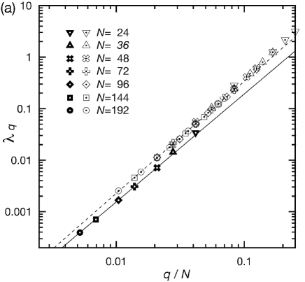
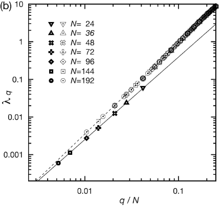
Figure 1: Log-log plots of (a) $\lambda^{(1)}_{q}$ versus $q/N$ and (b) $\lambda^{\rm(LA)}_{q}$ versus $q/N$ for the single ring polymer with the trivial knot, where $N=24$, $36$, $48$, $72$, $96$, $144$ and $192$. For each value of $N$, the solid symbols represent the relaxation rates for $q=1$ and the open symbols represent those for $q>1$. In each figure, the solid line represents the result of the least square fit of the data points for $q=1$ with $N=48$–$192$ to a straight line and the broken line represents that for $q>1$ with $q/N\leq 0.05$.

The behaviors of $\lambda^{\rm(LA)}_{q}$ in Fig. 1(b) are qualitatively similar to those of $\lambda^{(1)}_{q}$ in Fig. 1(a), although each value of $\lambda^{\rm(LA)}_{q}$ does not quantitatively agree with the corresponding value of $\lambda^{(1)}_{q}$, in contrast to the case of a single linear polymer.[23, 24] In each of Figs. 1(a) and 1(b), the data points for $q=1$ and those for $q>1$ seem to fall on two different straight lines at small values of $q/N$. This suggests the power law behaviors

$$\lambda^{(*)}_{q}\simeq\left\{\begin{array}[]{lcl}\displaystyle A^{(*)}_{1}\left(\frac{1}{N}\right)^{x^{(*)}_{1}}&{\rm for}&q=1,\vskip 12.0pt plus 4.0pt minus 4.0pt\\ \displaystyle A^{(*)}_{>1}\left(\frac{q}{N}\right)^{x^{(*)}_{>1}}&{\rm for}&q>1,\end{array}\right.$$ (14)

where the superscript $(*)$ denotes $(1)$ or ${\rm(LA)}$. The amplitudes and exponents in eq. (14) are estimated by the least square fit of the data points to a straight line in the log-log plot: $A^{(*)}_{1}$ and $x^{(*)}_{1}$ are estimated from the data points for $q=1$ with $N=48$–$192$; $A^{(*)}_{>1}$ and $x^{(*)}_{>1}$ are estimated from the data points for $q>1$ with $q/N\leq 0.05$. The estimated parameters for the relaxation rates $\lambda^{(1)}_{q}$ are given by $A^{(1)}_{1}\simeq 24.0$, $x^{(1)}_{1}\simeq 2.10$, $A^{(1)}_{>1}\simeq 50.2$ and $x^{(1)}_{>1}\simeq 2.17$. The exponents $x^{(1)}_{1}$ and $x^{(1)}_{>1}$ are similar to that for a linear polymer chain $2\nu+1\simeq 2.18$.[2, 23, 24] The separation of the power law dependences for $q=1$ and $q>1$ is attributed to the topological constraints, because no such separation appears for a single linear polymer[23, 24] and an ideal single ring polymer,[33] which have no excluded volume interaction. A similar separation of the power law dependences of the relaxation rates has been observed for a single linear polymer trapped in an array of obstacles in two dimensions.[27] The parameters for $\lambda^{\rm(LA)}_{q}$ are estimated as $A^{\rm(LA)}_{1}\simeq 60.9$, $x^{\rm(LA)}_{1}\simeq 2.19$, $A^{\rm(LA)}_{>1}\simeq 214$ and $x^{\rm(LA)}_{>1}\simeq 2.39$. Note that the relations $x^{(*)}_{1}<x^{(*)}_{>1}$ and $A^{(*)}_{1}<A^{(*)}_{>1}$ hold for both $\lambda^{(1)}_{q}$ and $\lambda^{\rm(LA)}_{q}$. It follows from the relations that the two straight lines in the log-log plot, which correspond to the power law behaviors for $q=1$ and $q>1$, intersects at a small value of $q/N$. This suggests that the two power law behaviors for $q=1$ and $q>1$ are only apparent and eventually merge into a single power law behavior $\lambda^{(*)}_{q}\propto(q/N)^{X}$ with $X=2\nu+1$ at sufficiently small values of $q/N$.

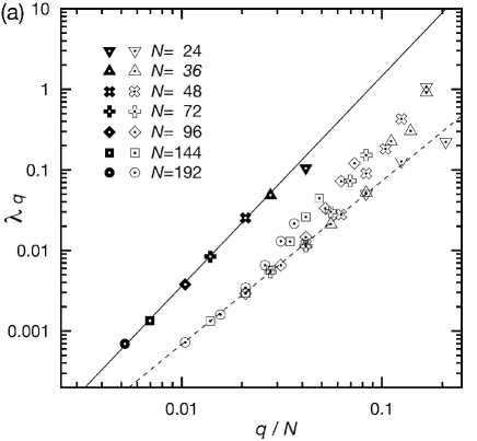
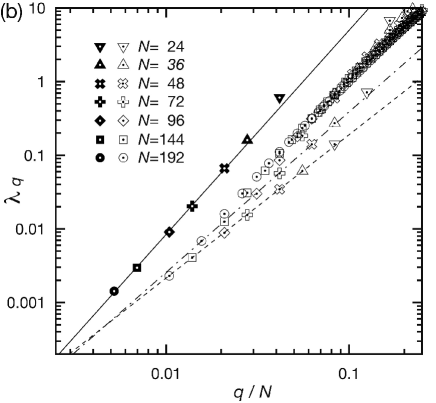
Figure 2: Log-log plots of (a) $\lambda^{(1)}_{q}$ versus $q/N$ and (b) $\lambda^{\rm(LA)}_{q}$ versus $q/N$ for the single ring polymer with the trefoil knot, where $N=24$, $36$, $48$, $72$, $96$, $144$ and $192$. For each value of $N$, the solid symbols represent the relaxation rates for $q=1$ and the open symbols represent those for $q>1$. In each figure, the solid line represents the result of the least square fit of data points for $q=1$. The broken line represents that for $q=2$ and $3$ in (a) and that for $q=2$ in (b). The dash-dotted line in (b) represents that for $q=3$. The data points for $N=48$–$192$ are used for each fit.

In Figures 2(a) and 2(b), the $q/N$-dependences of $\lambda^{(1)}_{q}$ and $\lambda^{\rm(LA)}_{q}$ are shown, respectively, for the ring polymer with the trefoil knot by a log-log plot, where the number of segments $N=24$, $36$, $48$, $72$, $96$, $144$ and $192$. In the same way as in Fig. 1, although values of $\lambda^{\rm(LA)}_{q}$ in Fig. 2(b) do not quantitatively agree with those of $\lambda^{(1)}_{q}$ in Fig. 2(a), the behaviors of $\lambda^{\rm(LA)}_{q}$ are qualitatively similar to those of $\lambda^{(1)}_{q}$. In Fig. 2(a), the data points for $q=1$ and those for $q=2$ and $3$ seem to fall on two different straight lines for small values of $q/N$, while the data points for $q=1$, those for $q=2$ and those for $q=3$ seem to fall on three different straight lines in Fig. 2(b). Therefore, we assume the power law behaviors

$$\lambda^{(*)}_{q}\simeq\begin{array}[]{lcl}\displaystyle A^{(*)}_{q}\left(\frac{q}{N}\right)^{x^{(*)}_{q}}&{\rm for}&q=\mbox{$1$, $2$ and $3$}\end{array}$$ (15)

and estimate $A^{(*)}_{q}$ and $x^{(*)}_{q}$ by the least square fit of the data points for each value of $q$ with $N=48$–$192$ to a straight line in the log-log plot. The parameters for $\lambda^{(1)}_{q}$ are estimated as $A^{(1)}_{1}\simeq 591$, $x^{(1)}_{1}\simeq 2.61$, $A^{(1)}_{2}\simeq 7.54$, $x^{(1)}_{2}\simeq 2.02$, $A^{(1)}_{3}\simeq 7.73$ and $x^{(1)}_{3}\simeq 2.04$. As expected, the relations $A^{(1)}_{2}\simeq A^{(1)}_{3}$ and $x^{(1)}_{2}\simeq x^{(1)}_{3}$ hold, which suggests that the relaxation rates $\lambda^{(1)}_{q}$ for $q=2$ and $3$ follow the same power law

$$\lambda^{(1)}_{q}\simeq\begin{array}[]{lcl}\displaystyle A^{(1)}_{2,3}\left(\frac{q}{N}\right)^{x^{(1)}_{2,3}}&{\rm for}&q=\mbox{$2$ and $3$}.\end{array}$$ (16)

The least square fit of the data points for $q=2$ and $3$ with $N=48$–$192$ gives $A^{(1)}_{2,3}\simeq 7.38$ and $x^{(1)}_{2,3}\simeq 2.02$. The parameters for $\lambda^{\rm(LA)}_{q}$ are estimated as $A^{\rm(LA)}_{1}\simeq 2.97\times 10^{3}$, $x^{\rm(LA)}_{1}\simeq 2.77$, $A^{\rm(LA)}_{2}\simeq 16.8$, $x^{\rm(LA)}_{2}\simeq 1.95$, $A^{\rm(LA)}_{3}\simeq 58.8$ and $x^{\rm(LA)}_{3}\simeq 2.18$. The estimated values of $A^{\rm(LA)}_{2}$, $x^{\rm(LA)}_{2}$, $A^{\rm(LA)}_{3}$ and $x^{\rm(LA)}_{3}$ lead to the intersection of the two straight lines for $q=2$ and $3$ at $(q/N)\simeq 4.3\times 10^{-3}$, which suggests that the two apparent power law behaviors merge into a single power law behavior at small values of $q/N$ in the same way as $\lambda^{(1)}_{q}$ with $q=2$ and $3$ follows the power law (16). In Fig. 2(a), the data points of $\lambda^{(1)}_{q}$ for $q=4$ with $N=96,144$ and $192$ seem to fall on the same straight line as the data points for $q=2$ and $3$ fall on. This suggests that the power law behavior like eq. (16) is obeyed by not only for $q=2$ and $3$ but for all values of $q>1$ at sufficiently small values of $q/N$. Moreover, the parameters $A^{(1)}_{1}$, $x^{(1)}_{1}$, $A^{(1)}_{2,3}$ and $x^{(1)}_{2,3}$, which satisfy $x^{(1)}_{2,3}<x^{(1)}_{1}$ and $A^{(1)}_{2,3}<A^{(1)}_{1}$, lead to the intersection of the two straight lines corresponding to the power law dependences for $q=1$ and $q=2$ and $3$ at $q/N\simeq 5.7\times 10^{-4}$. This suggests that the two apparent power law behaviors for $q=1$ and $q>1$ merge into a single power law behavior at small values of $q/N$.

As in the case of the trivial knot, the separation of the power law dependences of $\lambda^{(1)}_{q}$ for $q=1$ and $q=2$ and $3$ appears for the trefoil knot and the separation is attributed to the topological constraints. The pattern of the separation for the trefoil knot is, however, different from that for the trivial knot. In the case of the trefoil knot, $A^{(1)}_{1}>A^{(1)}_{2,3}$ and $x^{(1)}_{1}>x^{(1)}_{2,3}$ hold, while $A^{(1)}_{1}<A^{(1)}_{>1}$ and $x^{(1)}_{1}<x^{(1)}_{>1}$ hold for the trivial knot: In Fig. 2(a), the straight line corresponding to the power law dependence for $q=1$ lies above that for $q=2$ and $3$, while the straight line for $q=1$ is located below that for $q>1$ in Fig. 1(a). The separation of the power law dependences for the trefoil knot leads to the following characteristic behavior of the relaxation rates. As $N$ increases, the wave number $q=q_{\rm min}$ which gives the slowest relaxation rate $\lambda^{(1)}_{q}$ for each $N$ changes from $q_{\rm min}=2$ for $N\leq 96$ to $q_{\rm min}=1$ for $N\geq 144$. Because $\lambda^{\rm(LA)}_{q}$ given by eq. (12) shows the same crossover in Fig.  2(b), the crossover in $\lambda^{\rm(1)}_{q}$ can be considered to correspond to the the crossover in $\langle\hat{\mib{R}}_{q}\cdot\hat{\mib{R}}_{-q}\rangle$: The largest $\langle\hat{\mib{R}}_{q}\cdot\hat{\mib{R}}_{-q}\rangle$ for each $N$ is given by $q=2$ for small values of $N$ and $q=1$ for large values of $N$. Because $\langle\hat{\mib{R}}_{q}\cdot\hat{\mib{R}}_{-q}\rangle$ roughly corresponds to the mean square of the end-to-end distance of a partial chain with $N/(2q)$ segments as mentioned before, the crossover indicates that the end-to-end distance of a partial chain with $N/2$ segments is shorter than that with $N/4$ segments for small values of $N$ and is longer for large values of $N$. This change can be seen in Fig. 3, which shows the longest end-to-end vector of a partial chain with $N/2$ segments and that with $N/4$ segments in snapshots of the configurations of a ring polymer with the trefoil knot for $N=24$ and $N=192$. The longest end-to-end vector of a partial chain with $N/2$ segments is shorter than that with $N/4$ segments for $N=24$ and is longer for $N=192$.

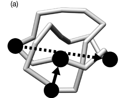
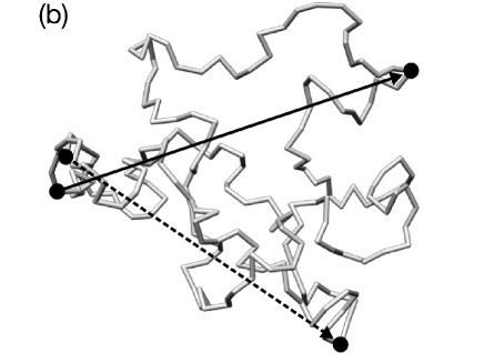
Figure 3: Snapshots of the configurations of the ring polymer with the trefoil knot for (a) $N=24$ and (b) $N=192$. The longest end-to-end vector of a partial chain with $N/2$ segments and that with $N/4$ segments are shown as solid and broken arrows, respectively. In each figure, the plane of perspective projection is parallel to the first and second principal axes of the moment of inertia tensor for the four end segments of the two end-to-end vectors.

In Fig. 3, the ring polymer with the trefoil knot is in a “uniform” state, where the knotted part is expanded widely along the polymer, for $N=24$ and is in a “phase segregated” state, where the knotted part is localized to a part of the ring polymer and the rest of the ring polymer behaves like a ring polymer with the trivial knot, for $N=192$.[14, 15, 8] Thus, the crossover from the state with $q_{\rm min}=2$ to that with $q_{\rm min}=1$ corresponds to the localization of the knotted part to a part of the ring polymer. The localization of the knotted part is considered to be driven by the entropy gained by the unknotted part which surpasses the entropy lost by the knotted part.

The localization of the knotted part of the ring polymer with the trefoil knot suggests that the proportion of the knotted part to the remainder part, which behaves like a ring polymer with the trivial knot, decreases as $N$ increases. Therefore, the behavior of the relaxation rates of the ring polymer with the trefoil knot is expected to approach that with the trivial knot as $N$ increases. From Figs. 1(a) and 2(a), it can be seen that $\lambda^{(1)}_{1}$ for the trefoil knot approaches that for the trivial knot from above as $N$ increases. In contrast, $\lambda^{(1)}_{q}$ with $q=2$ and $3$ for the trefoil knot approach $\lambda^{(1)}_{q}$ with $q>1$ for the trivial knot from below. As discussed above, for each of the trivial and the trefoil knots, the $q/N$-dependence of $\lambda^{(1)}_{q}$ is expected to show a single power law behavior at small values of $q/N$. Therefore, it is expected that the $q/N$-dependence of $\lambda^{(1)}_{q}$ shows the same single power law behavior at small values of $q/N$ independently of the knot type for sufficiently large values of $N$.

4 Summary and Discussion

In this paper, the relaxation rates of a single ring polymer with the trivial knot and the trefoil knot are studied through Brownian dynamics simulations for various values of the number of the segments of the ring polymer $N$. In the case of a single ring polymer, each relaxation mode is associated with a wave number $q$ because the ring polymer has the translational invariance along the polymer chain. The slowest relaxation rate $\lambda^{(1)}_{q}$ for each wave number $q$ is estimated by the least square fit of $\hat{C}_{q}(t)$ given by eq. (7) to the double exponential decay (11). The linearization approximation $\lambda^{\rm(LA)}_{q}$ to $\lambda^{(1)}_{q}$ is also estimated from the static correlation $\hat{C}_{q}(0)$ on the basis of eq. (12). The behavior of the distribution of $\lambda^{\rm(LA)}_{q}$ is qualitatively similar to that of $\lambda^{(1)}_{q}$, although each value of $\lambda^{\rm(LA)}_{q}$ is larger than the corresponding value of $\lambda^{(1)}_{q}$. Thus, in the case of a single ring polymer, the linearization approximation is useful for studying the behavior of the relaxation rate distribution qualitatively.

For the trivial knot, the relaxation rate $\lambda^{(1)}_{q}$ appears to behave as $A^{(1)}_{1}(1/N)^{x^{(1)}_{1}}$ for $q=1$ and $A^{(1)}_{>1}(q/N)^{x^{(1)}_{>1}}$ for $q>1$ at small values of $q/N$, where $A^{(1)}_{1}<A^{(1)}_{>1}$ and ${x^{(1)}_{1}}<{x^{(1)}_{>1}}$. The exponents ${x^{(1)}_{1}}$ and ${x^{(1)}_{>1}}$ are similar to that found for a single linear polymer chain. Even in the case of the trivial knot, the effect of the topological constraints appears as the separation of the power law dependences of $\lambda^{(1)}_{1}$ on $q/N$ for $q=1$ and $q>1$.

In the case of the trefoil knot, the topological constraints causes the separation of the power law dependences of $\lambda^{(1)}_{q}$ for $q=1$ and $q=2$ and $3$ as in the case of the trivial knot. In this case, the amplitudes and the exponents of the power law behaviors $\lambda^{(1)}_{1}\simeq A^{(1)}_{1}(1/N)^{x^{(1)}_{1}}$ for $q=1$ and $\lambda^{(1)}_{q}\simeq A^{(1)}_{2,3}(q/N)^{x^{(1)}_{2,3}}$ for $q=2$ and $3$ satisfy the relations $A^{(1)}_{1}>A^{(1)}_{2,3}$ and $x^{(1)}_{1}>x^{(1)}_{2,3}$, which is different from the case of the trivial knot. As the consequence of the separation of the power law behaviors, the wave number $q=q_{\rm min}$, which gives the slowest relaxation rate $\lambda^{(1)}_{q}$ for each $N$, is given by $q_{\rm min}=2$ for small values of $N$ and $q_{\rm min}=1$ for large values of $N$. This crossover corresponds to the change of the structure of the ring polymer from a state for small $N$, where the knotted part is extended along the ring polymer, to another state for large $N$, where the knotted part is localized to a part of the ring polymer and the rest of the ring polymer behaves like the ring polymer with the trivial knot. It is expected from the localization of the knotted part and the estimated parameters of the power law behaviors that the separated power law behaviors of the relaxation rates for the trivial knot and the trefoil knots eventually merge into a single power law behavior in the limit of $N\to\infty$, where the effects of the topological constraints vanish.

In this paper, we only consider the single ring polymers with the trivial knot and the trefoil knot, which are the simplest knots. Even for these simple knots, the effects of the topological constraints on the relaxation rate distribution are clearly observed. Therefore, it is interesting to study the relaxation rates distribution of single ring polymers with more complicated knots or ring polymers with links. The study in this direction is in progress. The topological effects seem to vanish in the limit that the number of the segments of the ring polymer goes to infinity because of the localization of the knotted part. The study of the localization of the knotted part of a single ring polymer is also in progress by using the average structure of the ring polymer defined self-consistently as the average structure of all the sampled structures, which are translated and rotated to minimize the mean square displacement from the average structure itself.

References

- [1] P. G. de Gennes: Scaling Concepts in Polymer Physics (Cornell University Press, Ithaca, 1984).
- [2] M. Doi and S. F. Edwards: The Theory of Polymers Dynamics (Oxford University Press, Oxford, 1986).
- [3] K. Hagita and H. Takano: J. Phys. Soc. Jpn. 71 (2002) 673.
- [4] K. Hagita and H. Takano: J. Phys. Soc. Jpn. 72 (2003) 1824 and references therein.
- [5] L. H. Kauffman: Knots and Physics (World Scientific, Singapore, 1993).
- [6] J. des Cloizeaux: J. Phys. (Paris) Lett. 42 (1981) L433.
- [7] J. M. Deutsch: Phys. Rev. E 59 (1999) R2539.
- [8] A. Y. Grosberg: Phys. Rev. Lett. 30 (2000) 3858.
- [9] T. Deguchi and K. Tsurusaki: Phys. Rev. E 55 (1997) 6245.
- [10] M. K. Shimamura and T. Deguchi: Phys. Rev. E 64 (2001) 020801(R).
- [11] M. K. Shimamura and T. Deguchi: J. Phys. A 35 (2002) L241.
- [12] M. K. Shimamura and T. Deguchi: Phys. Rev. E 65 (2002) 051802.
- [13] H. Matsuda, A. Yao, H. Tsukahara, T. Deguchi, K. Furuta and T. Imai: Phys. Rev. E 68 (2003) 011102.
- [14] E. Orlandini, M. C. Tesi, E. J. Janse van Rensburg and S. G. Whittington: J. Phys. A 31 (1988) 5953.
- [15] E. J. Janse van Rensburg and S. G. Whittington: J. Phys. A 24 (1991) 3935.
- [16] S. R. Quake: Phys. Rev. Lett. 73 (1994) 3317.
- [17] P.-Y. Lai: Phys. Rev. E 66 (2002) 021805.
- [18] P.-Y. Lai, Y.-J. Sheng and H.-K. Tsao: Phys. Rev. Lett. 87 (2001) 175503.
- [19] S. A. Wasserman and N. R. Cozzarelli: Science 232 (1986) 951.
- [20] S. Y. Shaw and J. C. Wang: Science 260 (1993) 533.
- [21] A. Stasiak, V. Katritch, J. Bednar, D. Michoud and J. Dubochet: Nature 384 (1996) 122.
- [22] H. Takano and S. Miyashita: J. Phys. Soc. Jpn. 64 (1995) 3688.
- [23] S. Koseki, H. Hirao and H. Takano: J. Phys. Soc. Jpn. 66 (1997) 1631.
- [24] H. Hirao, S. Koseki and H. Takano: J. Phys. Soc. Jpn. 66 (1997) 3399.
- [25] K. Hagita and H. Takano: J. Phys. Soc. Jpn. 68 (1999) 401.
- [26] K. Hagita, S. Koseki and H. Takano: J. Phys. Soc. Jpn. 68 (1999) 2144.
- [27] K. Hagita, D. Ishizuka and H. Takano: J. Phys. Soc. Jpn. 70 (2001) 2897.
- [28] P. E. Rouse, Jr.: J. Chem. Phys. 21 (1953) 1272.
- [29] B. H. Zimm: J. Chem. Phys. 24 (1956) 269.
- [30] G. S. Grest and K. Kremer: Phys. Rev. A 33 (1986) 3628.
- [31] K. Kremer and G. S. Grest: J. Chem. Phys. 92 (1990) 5057.
- [32] K. Binder: Monte Carlo and Molecular Dynamics Simulations in Polymer Science (Oxford University Press, Oxford, 1995).
- [33] V. Bloomfield and B. H. Zimm: J. Chem. Phys. 44 (1966) 315.