Interplay between strong correlations and magnetic field in the
symmetric periodic Anderson model

Abstract

Magnetic field effects in Kondo insulators are studied theoretically, using a local moment approach to the periodic Anderson model within the framework of dynamical mean-field theory. Our main focus is on field-induced changes in single-particle dynamics and the associated hybridization gap in the density of states. Particular emphasis is given to the strongly correlated regime, where dynamics are found to exhibit universal scaling in terms of a field-dependent low energy coherence scale. Although the bare applied field is globally uniform, the effective fields experienced by the conduction electrons and the $f$-electrons differ because of correlation effects. A continuous insulator-metal transition is found to occur on increasing the applied field, closure of the hybridization gap reflecting competition between Zeeman splitting and screening of the $f$-electron local moments. For intermediate interaction strengths the hybridization gap depends non-linearly on the applied field, while in strong coupling its field dependence is found to be linear. For the classic Kondo insulator YbB₁₂, good agreement is found upon direct comparison of the field evolution of the experimental transport gap with the theoretical hybridization gap in the density of states.

I Introduction

Kondo insulator materials such as SmB₆, YbB₁₂ and Ce₃Bi₄Pt₃ have been of sustained interest to experimentalists and theorists for several decades grewe ; hewson ; aeppli ; fisk ; takabatake ; degiorgi ; peter . Interest in these system stems from their unusual properties, such as the small hybridization gap (of a few meV) and mixed valency, as well as the transition to metallic behavior with doping dopedki , application of pressure presski and magnetic field magki . The underlying qualitative origin of such rich behavior is the strong electronic correlation arising due to the localized and narrow $f$-orbitals of the rare earth atoms, which hybridize weakly with broad, essentially non-interacting conduction bands.

A quantitative understanding of the dynamics and transport properties of these materials has not however been easy to achieve. A principal stumbling block in this regard has been the theoretical treatment of localized and itinerant fermionic degrees of freedom on a comparable footing. Much progress has been made in recent years with the advent of dynamical mean field theory (DMFT) vollhard ; jarrell ; kotliar ; gebhard , within which generic lattice-fermion models such as the Hubbard or the periodic Anderson model have found approximate solutions, and quantitative agreement with experiments has also been obtained raja_ki ; kotliar . Within DMFT vollhard ; jarrell ; kotliar ; gebhard , a lattice fermion model is mapped onto an effective single-site correlated impurity which hybridizes with a self-consistent conduction electron bath. Thus, various techniques such as the numerical renormalization group, exact diagonalization, diagrammatic perturbation theory based approaches, quantum Monte Carlo and many others that have, in the past, been developed to handle the many-body single-impurity problem, have now been adapted and modified for use within the DMFT framework vollhard ; jarrell ; kotliar ; gebhard . One such recent technique is the local moment approach (LMA) lmaintro ; NLDSR ; lmaff ; lmanrg ; victoria ; raja_ki ; rajahf ; epjb , which has been shown to be powerful not only in the context of single-impurity systems lmaintro ; lmaff ; lmanrg ; NLDSR , but also for lattice-based heavy fermion systems raja_ki ; rajahf ; victoria ; epjb when used in conjunction with DMFT. In this paper, we employ the LMA to understand the interplay of electronic correlations and an external magnetic field in Kondo insulator materials.

The generic model used to study Kondo insulator materials is the periodic Anderson model (PAM), which consists in physical terms of a correlated $f$-level in each unit cell hybridizing locally with a non-interacting conduction band. Magnetic field effects in these systems have been studied theoretically through the inclusion of a Zeeman term in the PAM saso ; lee . The observed insulator-metal transition magki has also been reproduced qualitatively in theoretical calculations saso . However, a detailed understanding of the changes in single-particle dynamics and the associated hybridization gap has on the whole been lacking, and a quantitative description of the experimentally observed field-induced behavior has not been achieved. We seek to bridge these gaps in this paper by studying the PAM with a Zeeman term using LMA+DMFT, and with particular emphasis on the strongly correlated (or strong coupling) regime. Our primary focus is on the field-induced changes in the single-particle dynamics and the associated hybridization gap in the density of states.

The outline of the paper is as follows: We begin in the next section with a brief description of the model (PAM), the DMFT framework and the LMA technique for the PAM in the presence of a magnetic field. In section 3 we present our theoretical results and their analysis. We also make comparison between theory and experiments on the classic Kondo insulator material $YbB$₁₂. Brief conclusions are given in section 4.

II Model and Formalism

The Hamiltonian for the PAM is given in standard notation by

$$H=-\sum_{\langle ij\rangle,\sigma}t_{ij}c_{i\sigma}^{\dagger}c_{j\sigma}^{\phantom{\dagger}}+\sum_{i\sigma}(\epsilon_{f}+\frac{U}{2}f_{i-\sigma}^{\dagger}f_{i-\sigma}^{\phantom{\dagger}})f_{i\sigma}^{\dagger}f_{i\sigma}^{\phantom{\dagger}}$$

$$+V\sum_{i\sigma}(f_{i\sigma}^{\dagger}c_{i\sigma}^{\phantom{\dagger}}+{\rm h.c})+{\epsilon}_{c}\sum_{i\sigma}c_{i\sigma}^{\dagger}c_{i\sigma}^{\phantom{\dagger}}$$ (1)

where the first term describes the kinetic energy of the noninteracting conduction ($c$) band due to nearest neighbour hopping $t_{ij}$. The second term refers to the $f$-levels with site energies ${\epsilon}_{f}$ and on–site repulsion $U$, while the third term describes the $c/f$ hybridization via the local matrix element $V$. The final term represents the $c$-electron orbital energy. Within DMFT vollhard ; jarrell ; kotliar ; gebhard , which is exact in the limit of infinite dimensions, the hopping term is scaled as $t_{ij}\propto t_{*}/\sqrt{Z_{c}}$, with coordination number $Z_{c}\rightarrow\infty$.In this paper we consider mainly the hypercubic lattice, for which the non-interacting density of states is a Gaussian kotliar ($\rho_{0}({\epsilon})=\exp(-{\epsilon}^{2}/t_{*}^{2})/\sqrt{\pi}t_{*})$. We also consider specifically the (particle-hole) symmetric PAM, which is the traditional limit employed to study Kondo insulators kotliar ; jarrell_ki ; raja_ki ; victoria ; saso ; lee ; shim ; sun ; pruschke ; faze . For the symmetric PAM the conduction band is located symmetrically about the Fermi level (i.e. ${\epsilon}_{c}=0$), while $\epsilon_{f}=-U/2$. This corresponds to half-filling of the $f$ and $c$-levels, i.e. $n_{f}=\sum_{\sigma}\langle f_{i\sigma}^{\dagger}f_{i\sigma}^{\phantom{\dagger}}\rangle=1$ and $n_{c}=\sum_{\sigma}\langle c_{i\sigma}^{\dagger}c_{i\sigma}^{\phantom{\dagger}}\rangle=1$ for all $U$. In this case the system is an insulator for all interaction strengths $U$ (in the absence of a magnetic field), with a corresponding gap in the single-particle spectra. The symmetric PAM in the absence of a magnetic field has been studied quite comprehensively within the DMFT framework, see e.g. kotliar ; jarrell ; victoria ; raja_ki ; shim ; jarrell_ki ; sun .

Within DMFT, the lattice fermion model maps onto an effective, correlated single-site impurity hybridizing self-consistently with a conduction electron bath vollhard ; jarrell ; kotliar ; gebhard . The self energy is thus spatially local, i.e. momentum independent. Thus, the problem is simplified to a great extent. Nevertheless, the problem remains non-trivial because the impurity model is as yet unsolved for an arbitrary hybridization. As mentioned in the introduction, the local moment approach lmaintro has been successful in describing the single impurity Anderson model lmaintro ; lmaff ; lmanrg ; NLDSR as well as in understanding the PAM within DMFT raja_ki ; rajahf ; victoria ; epjb . Here we extend the approach to encompass finite magnetic fields in the symmetric PAM, enabling study of magnetic field effects in Kondo insulators.

The local moment approach begins with the symmetry broken mean field state (unrestricted Hartree Fock, UHF). Dynamical self energy effects are then built in through the inclusion of transverse spin fluctuations for each of the symmetry broken states. The most important idea underlying the LMA at $T=0$ is that of symmetry restoration lmaintro ; NLDSR ; victoria : self-consistent restoration of the broken symmetry inherent at pure mean field level, arising in physical terms via dynamical tunneling between the locally degenerate mean-field states, and in consequence ensuring correct recovery of the local Fermi liquid behavior that reflects adiabatic continuity in $U$ to the non-interacting limit. The reader is referred to our earlier papers raja_ki ; victoria for full details of the formalism and implementation of the zero-field LMA for the PAM.

In the presence of a global magnetic field, the degeneracy between the mean field solutions lmaintro (labeled as A and B corresponding to $+|\mu|$ and -$|\mu|$) found at the mean field level is lifted, and only one solution as determined by $sgn(h)$ remains lmaff . Here, we consider explicitly $h>0$ for which only the ‘A’ solution survives. For $h\neq 0$ the bare electronic energy levels, $\epsilon_{\alpha}$ for $\alpha=c$ and $f$, are of course split via the Zeeman effect. The modified energy levels are given by ${\epsilon}_{\alpha\sigma}={\epsilon}_{\alpha}-\sigma h_{\alpha}$ with $h_{\alpha}=\tfrac{1}{2}g_{\alpha}\mu_{B}H$ (and $\sigma=\pm$ for $\uparrow/$$\downarrow$ spins), where $\mu_{B}$ is the Bohr magneton, $g_{\alpha}$ the Lande g-factor and $B$ the magnetic field. Although $g_{f}\neq g_{c}$ in general, for simplicity we set $g_{f}=g_{c}=g$ i.e. we consider the application of a uniform magnetic field $h\equiv h_{c}=h_{f}$ to both $c$ and $f$-levels. The local (site-diagonal) Green functions for the $c$- and $f$-levels may be expressed using the Feenberg renormalized perturbation theory feenberg ; economou as

$$G_{A\sigma}^{c}(\omega;h) = [\omega^{+}+\sigma h-\frac{V^{2}}{\omega^{+}+\sigma h-\tilde{\Sigma}_{fA\sigma}(\omega;h)}$$ (2)

$$-S_{A\sigma}[G_{A\sigma}^{c}(\omega;h)]]^{-1}$$

$$G_{A\sigma}^{f}(\omega;h) = [\omega^{+}+\sigma h-\tilde{\Sigma}_{fA\sigma}(\omega;h)-$$ (3)

$$\frac{V^{2}}{\omega^{+}+\sigma h-S_{A\sigma}[G_{A\sigma}^{c}(\omega;h)]}]^{-1}.$$

where $\omega^{+}=\omega+isgn(\omega)0^{+}$. Here $S_{A\sigma}$ is the Feenberg self energy, a functional solely of $G_{A\sigma}^{c}$, given by

$$S_{A\sigma}({\omega};h)=\gamma_{A\sigma}({\omega};h)-\frac{1}{{\rm{H}}[\gamma_{A\sigma}({\omega};h)]}\\$$ (4)

with

$$\gamma_{A\sigma}({\omega};h)=\omega^{+}+\sigma h-\frac{V^{2}}{\omega^{+}+\sigma h-\tilde{\Sigma}_{fA\sigma}(\omega;h)}$$ (5)

and the Hilbert transform ${\rm H}[z]$ defined as

$${\rm{H}}[z]=\int^{\infty}_{-\infty}\frac{\rho_{0}({\epsilon})\,d{\epsilon}}{z-{\epsilon}}\,$$ (6)

such that $G^{c}_{A\sigma}({\omega};h)=H[\gamma_{A\sigma}]$.

Dropping the ‘A’ subscript for clarity, the spin-summed Green functions are denoted by $G^{\alpha}(\omega;h)=\tfrac{1}{2}\sum_{\sigma}G_{\sigma}^{\alpha}(\omega;h)$ ($\alpha=c,f$), with corresponding spectral functions $D^{\alpha}(\omega;h)=-\frac{1}{\pi}sgn(\omega){\rm{Im}}G^{\alpha}(\omega;h)$. Within the LMA the $f$-electron self energies $\tilde{\Sigma}_{f\sigma}(\omega;h)$are familiarly separated into a static mean-field contribution plus a dynamical part $\Sigma_{f\sigma}(\omega;h)$ lmaintro ; raja_ki ; victoria ,

$$\tilde{\Sigma}_{f\sigma}(\omega;h)=-\frac{\sigma}{2}U|\bar{\mu}(h)|+\Sigma_{f\sigma}(\omega;h)$$ (7)

where $|\bar{\mu}(h)|$ is the UHF local moment. We approximate the dynamical part of the self energy by the usual non-perturbative class of diagrams retained in practice by the LMA (as shown in figure 1), which may be expressed mathematically at zero temperature lmaintro ; raja_ki ; victoria as

$$\Sigma_{f\sigma}(\omega;h)=U^{2}\int_{-\infty}^{\infty}\frac{d\omega_{1}}{2\pi i}\;{\cal{G}}_{-\sigma}(\omega-\omega_{1};h)\Pi^{-\sigma\sigma}(\omega_{1};h).$$ (8)

Here the host/medium Green function ${\cal{G}}_{\sigma}$ (denoted by the double-lined propagator in figure 1) is defined by

$${\cal{G}}_{\sigma}({\omega};h)^{-1}=G^{f}_{\sigma}({\omega};h)^{-1}+\Sigma_{f\sigma}({\omega};h)\,.$$ (9)

$\Pi^{-\sigma\sigma}(\omega;h)$ denotes the transverse spin polarization propagator (shown shaded in figure 1), which in the random phase approximation employed is expressed as $\Pi^{+-}=\,^{0}\!\Pi^{+-}/(1-U\,^{0}\!\Pi^{+-})$. The bare polarization propagator ${}^{0}\!\Pi^{+-}(\omega;h)$ is expressed in terms of mean-field propagators victoria ; raja_ki $\{g^{\alpha}_{\sigma}({\omega};h)\}$ (in which only the static Fock contribution to the self-energies occurs).

Figure 1: Principal contribution to the LMA $\{\Sigma_{f\sigma}(\omega)\}$. Wavy lines denote U. See text for details.

For $h=0$ the symmetry restoration (SR) condition for the symmetric PAM is given by victoria ; raja_ki $\tilde{\Sigma}_{f\sigma}(\omega=0;h=0)=0$ (independent of spin $\sigma$, since by particle-hole symmetry $\tilde{\Sigma}_{f\sigma}(\omega;h)=-\tilde{\Sigma}_{f-\sigma}(-\omega;h)$), i.e. by

$$\Sigma_{f\uparrow}({\omega}=0;h=0)=U|\bar{\mu}|/2.$$ (10)

Satisfaction of the SR condition ensures adiabatic continuity (in $U$) to the non-interacting limit victoria ; raja_ki of the hybridization-gap insulator (the system being in that sense a generalized Fermi liquid victoria ; raja_ki ); and as expected the system remains insulating, with a gap in the single-particle spectra, for all interactions $U\geq 0$.

The practical implementation of the above procedure is carried out as follows raja_ki ; victoria ; epjb , in which the numerical procedure is simplified by keeping $x=\tfrac{1}{2}U|\mu|$ fixed, while varying $U$ to satisfy the symmetry restoration condition. We begin with an $h=0$ calculation for a given $x$. (i) The mean-field Green functions $g^{\alpha}_{\sigma}({\omega};h)$ are obtained from equations (2-7) by retaining only the static part of the self energy. (ii) These Green functions are then used to construct the bare polarization bubble ${}^{0}\!\Pi^{+-}$. (iii) The DMFT iterative procedure starts with a specific dynamical self energy, obtained either as a guess or from the previous iteration, which is substituted into equations (2-7) to get the $c$- and $f$- Green functions. (iv) The host/medium Green function ${\cal{G}}_{\sigma}({\omega};h)$ is obtained through equation (9). (v) The transverse spin polarization propagator $\Pi^{+-}$ is computed for a given $U$ and along with ${\cal{G}}_{\sigma}({\omega};h)$, substituted in equation (8) to determine the ${\omega}=0$ self energy for a given $U$; (vi) The SR condition (equation (10)) is checked, and if found not to be satisfied, $U$ is varied and step (v) is repeated until the SR condition is satisfied. (vii) Upon restoration of the broken spin symmetry, the corresponding $U$ is obtained and equation (8) may then be used to get the full dynamical self energy at all frequencies. (viii) The new self energy is fedback in the first step of the DMFT procedure (step (iii)) and the iterations are continued until full self-consistency is achieved. For finite fields the same procedure is adopted except that SR is no longer imposed lmaff (the $U$ found from SR at $h=0$ is naturally used for all $h>0$).

III Results and Discussion

Before discussing the interplay between interactions and magnetic fields in the symmetric PAM, we consider briefly two limiting cases. (i) First the non-interacting limit, $U=0$, with $h\neq 0$; and secondly (ii) the interacting problem $U>0$ in the absence of a field. In the former case, the non-interacting $c$-spectrum for spin-$\sigma$ is given by

$$d^{c}_{0\sigma}({\omega};h)=\rho_{0}\left({\omega}+\sigma h-\frac{V^{2}}{{\omega}+\sigma h}\right)\,.$$

The spectral band edges are given by

$${\omega}+\sigma h-\frac{V^{2}}{{\omega}+\sigma h}=\pm W$$ (11)

where $2W$ is the full band-width of the non-interacting density of states $\rho_{0}(\omega)$. It is easy to see from this that for $h=0$ there is a hybridization gap at the Fermi level (denoted by $\Delta_{0}(0)$), which decreases with increasing field $h$ and eventually closes at a field value that is half of the zero field spectral gap, i.e.

$$\Delta_{0}(h)=\Delta_{0}(0)-2h.$$ (12)

Thus in the non-interacting limit, application of a magnetic field leads to an insulator-metal transition simply because of the rigid crossing of the up- and down-spin bands. We add here that the non-interacting Gaussian density of states characteristic of the hypercubic lattice (as considered explicitly below) is of course unbounded and as such does not possess ‘hard’ band edges. The field-induced insulator-metal transition in this case is thus strictly a crossover, although in practice the transition is ‘sharp’ as one would expect (see e.g. figure 5).

In the second limit, of finite interactions but zero field, the ground state remains gapped for all interaction strengths victoria , the hybridization gap $\Delta$ decreasing continuously with increasing $U$ from its non-interacting limit $\Delta_{0}(0)$. In the strong coupling, Kondo lattice regime of the model, universal scaling occurs raja_ki ; victoria ; shim ; pruschke ; faze in terms of an exponentially small low energy scale ${\omega}_{L}=ZV^{2}/t_{*}(\equiv\frac{1}{2}\Delta)$; $Z$ being the quasiparticle weight or mass renormalization factor, given by $Z=(1-\partial\Sigma_{f\sigma}(\omega)/\partial{\omega}|_{{\omega}=0})^{-1}$. The Green functions and their associated spectra depend solely on ${\tilde{\omega}}={\omega}/{\omega}_{L}$ in the universal scaling regime raja_ki ; victoria . Representative results for the zero-field density of states are shown in figure 2; where the main panels show the conduction band density of states, $t_{*}D^{c}({\omega})$ (solid lines), as a function of frequency, ${\omega}/t_{*}$. The right panels represent intermediate coupling ($U/t_{*}=1.2$), while the left panels are for strong coupling ($U/t_{*}=7.1$). The insets show a close-up of the low frequency spectra where the hybridization gap at the Fermi level (${\omega}=0$) is evident at both weak and strong coupling.

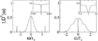
Figure 2: LMA conduction electron spectra for $h=0$, in strong coupling (left panel, $U/t_{*}=7.1$) and weaker coupling (right panel, $U/t_{*}=1.2$), with $V^{2}=0.2t_{*}^{2}$. Insets show the low frequency region of the respective main panels.

Now we consider both interactions and the field. In the strong coupling regime, in parallel to the $h=0$ limit, we expect universality to persist in terms of a field-dependent low energy scale, $\omega_{L}\equiv\omega_{L}(h)$. To derive explicitly the universal scaling form in the limit of low-frequencies (i.e. close to the Fermi level), we perform a simple low-frequency ‘quasiparticle expansion’ of the self energy, retaining only its real part ($\Sigma^{R}_{f\sigma}$) to leading order in $\omega$; i.e.

$$\Sigma^{R}_{f\sigma}({\omega};h)=\Sigma^{R}_{f\sigma}(0;h)-\left(\frac{1}{Z(h)}-1\right){\omega}\,$$ (13)

where $Z(h)=(1-\partial\Sigma^{R}_{f\sigma}(\omega;h)/\partial{\omega}|_{{\omega}=0})^{-1}$ is the field-dependent quasiparticle weight (independent of $\sigma$ since $\Sigma^{R}_{f\sigma}(\omega;h)=-\Sigma^{R}_{f-\sigma}(-\omega;h)$ by particle-hole symmetry).

Substituting equation (13) into equations (2-7), we find that the associated spectral functions are just renormalized versions of their non-interacting counterparts, being given by

$$D^{c}_{\sigma}({\omega};h) \stackrel{{\scriptstyle{\omega}\rightarrow 0}}{{\rightarrow}} \rho_{0}\left(-\frac{1}{{\tilde{\omega}}+\sigma{h_{e\!f\!\!f}}}\right)$$ (14)

$$D^{f}_{\sigma}({\omega};h) \stackrel{{\scriptstyle{\omega}\rightarrow 0}}{{\rightarrow}} \frac{t_{*}^{2}}{V^{2}}\frac{1}{({\tilde{\omega}}+\sigma{h_{e\!f\!\!f}})^{2}}~{}D^{c}_{\sigma}({\omega};h)$$ (15)

where ${\tilde{\omega}}={\omega}/{\omega}_{L}(h)$, and the low-energy scale $\omega_{L}(h)=Z(h)V^{2}/t_{*}$ is thus defined (in direct parallel to the $h=0$ limit). In obtaining equations (14,15) we have explicitly considered the strong coupling scaling regime, of finite $\tilde{\omega}=\omega/\omega_{L}(h)$ and $h/\omega_{L}(h)$ in the formal limit where the low-energy scale $\omega_{L}\rightarrow 0$ (so that ‘bare’ factors of $\omega\equiv\tilde{\omega}\omega_{L}$ or $h$ are thus neglected). ${h_{e\!f\!\!f}}$ in equations (14,15) is given by

$${h_{e\!f\!\!f}}=\left[h-\sigma\tilde{\Sigma}^{R}_{f\sigma}(0;h)\right]~{}\frac{t_{*}}{V^{2}}\,$$ (16)

(being independent of $\sigma$, by symmetry); or equivalently, using the symmetry restoration condition $\tilde{\Sigma}^{R}_{f\sigma}(0;0)=0$, by

$${h_{e\!f\!\!f}}=\left[h+\sigma\left(\tilde{\Sigma}^{R}_{f\sigma}(0;0)-\tilde{\Sigma}^{R}_{f\sigma}(0;h)\right)\right]\,\frac{t_{*}}{V^{2}}.$$ (17)

In physical terms, ${h_{e\!f\!\!f}}$ represents a dimensionless effective field, and its primary field-dependence arises from that of the interaction self-energy (the ‘bare’ factor of $h$ in equations (16) or (17) can of course be dropped in the strict scaling limit, although we retain it for clarity). In fact a leading order Taylor expansion of equation (16) or (17) gives ${h_{e\!f\!\!f}}=c\tilde{h}$, where $\tilde{h}=h/\omega_{L}(0)$ is the field rescaled in terms of the $h=0$ low energy scale $\omega_{L}(h=0)=Z(0)V^{2}/t_{*}$, and $c=Z(0)/\tilde{Z}$ ($\sim{\cal{O}}(1)$) with ${\tilde{Z}}=[1-\sigma(\partial\Sigma^{R}_{f\sigma}(0;h)/\partial h)_{h=0}]^{-1}$ thus defined. From this simple consideration we anticipate that ${h_{e\!f\!\!f}}$ is just a rescaled version of the bare magnetic field itself, and is on the order of $\tilde{h}=h/\omega_{L}(0)$ (as confirmed explicitly below, see figure 5).

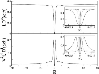
Figure 3: LMA spectra for the $c$-electrons (top panel, $t_{*}D^{c}(\omega;h)$) and $f$-electrons (bottom panel, $V^{2}t^{-1}_{*}D^{f}(\omega;h)$), for three parameter sets, each corresponding to a fixed ${h_{e\!f\!\!f}}=0.27$: $Ut_{*}/V^{2}=35,h/t_{*}=2.4\times 10^{-5}$(dashed), $Ut_{*}/V^{2}=30,h/t_{*}=7.4\times 10^{-5}$(dotted) and $Ut_{*}/V^{2}=25,h/t_{*}=2.3\times 10^{-4}$(solid). The insets show the spectra vs. ‘bare’ frequency, ${\omega}/t_{*}$. Main panel: The same spectra plotted vs. ${\tilde{\omega}}={\omega}/\omega_{L}(h)$ collapse to a common scaling form.

Equations (14) and (15) show that in strong coupling, the spectra $D^{c}(\omega;h)$ and $V^{2}D^{f}(\omega;h)$ should be universal functions of $\tilde{\omega}=\omega/\omega_{L}(h)$, for a fixed ${h_{e\!f\!\!f}}$. Thus, if distinct sets of model parameters in the strong coupling regime correspond to the same ${h_{e\!f\!\!f}}$, the spectra $D^{c}$ and $V^{2}D^{f}$ should collapse to the same scaling form as a function of ${\tilde{\omega}}$, independently of the bare parameters $U/t_{*}$ and $V/t_{*}$. That this is is so is illustrated in figure  3, where the top panel shows the full LMA $c$-electron spectra $t_{*}D^{c}$ for the hypercubic lattice, and the bottom panel the corresponding $f$-electron specta $(V^{2}/t_{*})D^{f}$. Three sets of spectra are shown, with parameters $Ut_{*}/V^{2}=35$ and $h/t_{*}=2.4\times 10^{-5}$(dashed), $Ut_{*}/V^{2}=30$ and $h/t_{*}=7.4\times 10^{-5}$ (dotted) and $Ut_{*}/V^{2}=25$ with $h/t_{*}=2.3\times 10^{-4}$(solid); in each case, ${h_{e\!f\!\!f}}$ ($=0.27$) is the same. The insets to the figure show that the spectra as a function of the ‘bare’ frequency ${\omega}/t_{*}$ are distinct. However when plotted vs. ${\tilde{\omega}}$ (as shown in the main panels), they are indeed seen to collapse to a single universal form.

The quasiparticle forms in equations (14,15) embody local Fermi liquid behavior and adiabatic continuity to the non-interacting limit. They give explicitly the leading low-frequency asymptotic behavior of the scaling spectra that must be satisfied by any ‘full’ theory. Direct comparison between the quasiparticle forms and the full LMA scaling spectra is shown in figure 4 for the $c$-electron spectra, and for two values of the effective field ${h_{e\!f\!\!f}}$ (one corresponding to a case where the system remains insulating, the other for a higher field where the system is metallic, as discussed below). It is indeed clear from the figure that the LMA correctly recovers the limiting quasiparticle form in the vicinity of the Fermi level. In physical terms it is also worth noting that the low frequency quasiparticle spectra are essentially those for the non-interacting limit, but with the local fields for $f$- and $c$-electrons replaced by $(V^{2}/t_{*}){h_{e\!f\!\!f}}$ and zero respectively. Hence, although the bare applied field is globally uniform, the effective local fields experienced by the $c$ and $f$ electrons are different because of correlation effects.

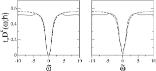
Figure 4: Full LMA $c$-electron scaling spectra (solid lines) are compared to the limiting quasiparticle form equation (14) (dashed lines). The left panel shows the scaling spectra for ${h_{e\!f\!\!f}}=0.27$ (where the system is an insulator) and the right panel for ${h_{e\!f\!\!f}}=0.51$ (metallic).

We turn now to the transition with increasing field from an insulating state characterised by a spectral gap straddling the Fermi level, to a metal with a finite density of states at $\omega=0$. Equations 14 and 15 may be used to obtain an estimate of the spectral band edges in strong coupling, and hence the gap as a function of the field. The band edges are given by

$$\frac{1}{{\tilde{\omega}}+\sigma{h_{e\!f\!\!f}}}=\pm W/t_{*}$$ (18)

with $2W$ the band-width of the non-interacting spectrum. From this the field-dependent gap in $D^{c}({\omega};h)$ or $D^{f}({\omega};h)$ follows as

$$\Delta(h)=2\left(1-{h_{e\!f\!\!f}}\frac{W}{t_{*}}\right)~{}\frac{Z(h)V^{2}}{W}\,.$$ (19)

This in turn implies an insulator to metal transition at a critical effective field ${h_{e\!f\!\!f}}$${}_{\!,c}$ that is on the order of unity ($\sim t_{*}/W$).

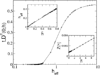
Figure 5: $c$-band spectrum at the Fermi level $D^{c}(0;h)$ in the strong coupling, universal regime as a function of ${h_{e\!f\!\!f}}$, showing a continuous insulator-metal transition at ${h_{e\!f\!\!f}}$${}_{\!,c}\simeq 0.36$. Top inset: shows the linear dependence of the effective field ${h_{e\!f\!\!f}}$ on $\tilde{h}=h/\omega_{L}(0)$ ($\omega_{L}(0)=Z(0)V^{2}/t_{*}$). Bottom inset: linear increase of the quasiparticle weight $Z(h)$ with increasing $\tilde{h}$.

The main panel in figure 5 shows the variation of the full LMA density of states at the Fermi level, $D^{c}(\omega=0;h)$ (calculated explicitly for $U/t_{*}=6.1,V^{2}/t_{*}^{2}=0.2$), as a function of ${h_{e\!f\!\!f}}$ on a log scale. Although the calculations are for a hypercubic lattice, with a strictly soft gap in its zero-field spectrum, the insulator-metal transition is seen in practice to be sharp; occurring at a critical ${h_{e\!f\!\!f}}$${}_{\!,c}\simeq 0.36$ that is indeed on the order of unity (we identify the critical field in practice from $t_{*}D^{c}(0;h_{c})\sim 10^{-3}$). On further increase of the field, $D^{c}(0;h)$ is seen from the figure to rise continuously, towards the high-field value of $1/\sqrt{\pi}t_{*}$ which is just the non-interacting dos value at the Fermi level.

The top inset to figure 5 shows the dependence of the effective field ${h_{e\!f\!\!f}}$ (equations (16,17)) on the scaled external field $\tilde{h}=h/\omega_{L}(0)$ (with $\omega_{L}(0)=Z(0)V^{2}/t_{*}$). ${h_{e\!f\!\!f}}$ is seen to be linear in $\tilde{h}$ (which behavior extends over a wide $\tilde{h}$ interval) and, as anticipated above, is of the same order as it: ${h_{e\!f\!\!f}}\simeq\tilde{h}/2$ as evident from the figure. The lower inset to the figure also shows the $\tilde{h}$-dependence of the quasiparticle weight $Z(h)$. It too is seen to increase linearly with field, implying a lowering of effective mass with an increase in field; and which behavior is consistent with a similar finding for the single impurity Anderson model lmaff .

The field-dependence of the full density of states is illustrated in figure 6, where we plot the (universal, strong coupling) conduction band density of states $D^{c}({\omega};h)$, as a function of the $\tilde{{\omega}}$, for various ${h_{e\!f\!\!f}}$. The solid curve ${h_{e\!f\!\!f}}=0$ represents the insulating ground state, while the dotted curve is for ${h_{e\!f\!\!f}}=0.38$, which is just above the insulator-metal transition, so the gap has closed. The remaining curves are for ${h_{e\!f\!\!f}}=1$ and ${h_{e\!f\!\!f}}=5$, showing metallic densities of states characterised by a finite spectral density $D^{c}(0;h)$ at the Fermi level.

Figure 6: Universal $c$-electron spectra from the LMA are shown as a function of ${\tilde{\omega}}=\omega/\omega_{L}$ for various fields: ${h_{e\!f\!\!f}}=0$ (solid), ${h_{e\!f\!\!f}}=0.38$ (dotted), ${h_{e\!f\!\!f}}=1$ (dashed) and ${h_{e\!f\!\!f}}=5$ (dot-dashed). The closure of the insulating gap with increasing field is evident.

In the non-interacting limit, $U=0$, the spectral gap closes linearly with the applied field as in equation 12, and the essential mechanism for the insulator-metal transition is obvious: Zeeman splitting moves the up- and down-spin bands rigidly, resulting in their crossing at a critical field, $h_{c0}/\Delta_{0}(0)=\tfrac{1}{2}$. This simple picture is naturally modified in the presence of correlations, $U>0$, where two essentially competing effects are operative. First, the tendency of the system to lower its energy by uniform (‘ferromagnetic’) spin polarization of the $c$- and $f$-electrons, i.e. the Zeeman effect, which alone operates in the non-interacting limit. However for $h=0$ in the presence of interactions, lattice-coherent Kondo singlet formation occurs, driven by local antiferromagnetic spin correlations between the $c$- and $f$-electrons. In the presence of both interactions and a field, Zeeman splitting thus in effect competes with local moment screening; and the field-dependence of the spectral gap is not a priori obvious.

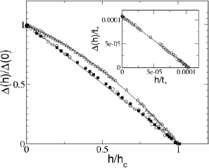
Figure 7: The field-dependent spectral gap scaled by the zero field gap, $\Delta(h)/\Delta(0)$, vs. $h/h_{c}$, for $U/t_{*}=1.2,V^{2}/t_{*}^{2}=0.2$ (triangles), $U/t_{*}=5.1,V^{2}/t_{*}^{2}=0.2$ (squares) and $U/t_{*}=6.1,V^{2}/t_{*}^{2}=0.2$ (circles). (The lines are best fits to the points.) Inset: the gap in units of $t_{*}$ vs. the bare field $h/t_{*}$.

LMA results for the spectral gap are shown in figure 7 where the field dependent gap scaled by the zero field gap, $\Delta(h)/\Delta(0)$, is plotted vs. $h/h_{c}$ for various interaction strengths. For intermediate coupling ($U/t_{*}=1.2,V^{2}/t_{*}^{2}=0.2$ (triangles)), the gap is seen to close non-linearly in the field and is best fit by a quadratic form. In the strong coupling regime by contrast (squares, $U/t_{*}=5.1,V^{2}/t_{*}^{2}=0.2$ and circles, $U/t_{*}=6.1,V^{2}/t_{*}^{2}=0.2$), linear behavior $\Delta(h)=\Delta(0)(1-h/h_{c})$ is obtained, similar to the non-interacting limit. In this case however, when $\Delta(h)$ is plotted directly vs. the bare field $h/t_{*}$ as shown in the inset of figure 7, the functional form obtained is $\Delta(h)=\Delta(0)-h$; showing that the field $h_{c}$ required to close the gap in strong coupling satisfies $h_{c}/\Delta(0)=1$, i.e. twice that required in the non-interacting limit, where $h_{c0}/\Delta_{0}(0)=\tfrac{1}{2}$. This result is physically natural, in view of the effective competition between Zeeman splitting and local moment screening discussed above.

Finally, we would like to make a comparison of our theoretical results to experiment. For the classic Kondo insulator $YbB_{12}$, the field dependence of the transport gap has been determined from low-temperature resistivity measurements magki (the leading low-$T$ behavior of the resistivity being $\rho(T)\propto\exp(-\Delta_{tr}/T)$ with $\Delta_{tr}\equiv\Delta_{tr}(h)$ the transport/activation gap). Since the transport gap is known theoretically raja_ki to be proportional to the spectral gap ($\Delta(0)\simeq 2\Delta_{tr}(0)$ raja_ki ), comparison to experiment may be made.

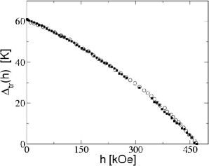
Figure 8: Comparison of the experimental magki transport gap in $YbB_{12}$ (opencircles) to the theoretical gap (filled squares), obtained as discussed in text. The theory is seen to describe well the functional form of the transport gap.

In our earlier work raja_ki where we compared zero-field transport properties of $YbB_{12}$ to theoretical results from the LMA, we concluded that $YbB_{12}$ belongs to the intermediate coupling regime (and as such lies outside the universal scaling regime). This is corroborated by the field-dependence of the transport gap, experimental results for which magki are shown as open circles in figure 8. The dependence of $\Delta_{tr}(h)$ on the field $h$ is clearly non-linear, which behavior we have found above to be characteristic of the intermediate coupling regime. To make comparison to experiment in this regime, specific model parameters must of course be specified, and here we choose $U/t_{*}=1.2,V^{2}/t_{*}^{2}=0.2$ (the essential results are quite insensitive to these particular values). The filled squares in figure 8 show the field dependence of the resultant theoretical spectral gap, compared directly to experiment with a simple multiplicative scaling of the $x$ and $y$ axes. The functional form of the theoretical gap is seen to be almost identical to that found experimentally, thus yielding good agreement between theory and experiment. Further, since the experimental $\Delta_{tr}(0)\simeq 60K$ (figure 8) then the spectral gap $\Delta(0)\simeq 2\Delta_{tr}(0)\simeq 120K$; and for the bare parameters considered we find $\Delta(0)=0.026t_{*}$. This in turn yields the estimate $t_{*}\simeq 0.4eV$, which is physically realistic and compatible with transfer integral values found through a band structure calculation saso_band .

IV Conclusion

The interplay between electronic correlations and an externally applied magnetic field in Kondo insulators has been considered in this paper. The symmetric periodic Anderson model, with a Zeeman term to account for the external magnetic field, has been studied within the dynamical mean field framework using a local moment approach. In the strong coupling Kondo lattice regime of the model, the local $c$- and $f$-electron spectral functions are found to exhibit universal scaling, being functions solely of $\omega/\omega_{L}$ (with $\omega_{L}(h)=Z(h)V^{2}/t_{*}$ the characteristic low-energy scale) for a given effective field ${h_{e\!f\!\!f}}$. Although the externally applied field is globally uniform, the effective local field experienced by the $c$- and $f$-electrons differs because of correlation effects. The zero-field spectral gap characteristic of Kondo insulators is found to close continuously, leading to a continuous insulator-metal transition at a critical applied field $h_{c}$. Field induced closure of the insulating gap is not simply a rigid band-crossing affair, but involves competition between local moment screening (reflecting correlation effects) and Zeeman spin-polarization. In the intermediate coupling regime the gap is found to close non-linearly with field, while in the strong coupling regime it closes linearly. Comparison of the theoretical gap with the transport gap measured in the intermediate coupling material $YbB_{12}$ yields good agreement, providing support to the scenario presented for the field-induced gap closure.

- (1) N. Grewe and F. Steglich F Handbook on the Physics and Chemistry of Rare Earths vol 14, ed K A Gschneider Jr and L L Eyring(Amsterdam: Elsevier) (1991).
- (2) A. C. Hewson, The Kondo Problem to Heavy Fermions(Cambridge: Cambridge University Press, 1993).
- (3) G. Aeppli and Z. Fisk, Comments Condens. Matter Phys. 16 155 (1992).
- (4) Z. Fisk et al, Physica B 223/224 409 (1996).
- (5) T. Takabatake et al, J. Magn. Magn. Mater. 177-181 277 (1998).
- (6) L. Degiorgi, Rev. Mod. Phys. 71 687 (1999).
- (7) Peter S. Riseborough, Adv. Phys. 49 257 (2000).
- (8) J. F. DiTusa, K. Friemelt, E. Bucher, G. Aeppli and A. P. Ramirez, Phys. Rev. Lett. 78 2831 (1997).
- (9) A. Barla et al, Phys. Rev. Lett. 94 166401 (2005).
- (10) K. Sugiyama, F. Iga, M. Kasaya, T. Kasaya, and M. Date, J. Phys. Soc. Japan 57, 3946 (1988).
- (11) A. Georges, G. Kotliar, W. Krauth, and M. Rozenberg, Rev. Mod. Phys. 68, 13 (1996).
- (12) D. Vollhardt, Correlated Electron Systems Vol. 9, ed. V. J. Emery (World Scientific, Singapore, 1993).
- (13) T. Pruschke, M. Jarrell, and J. K. Freericks, Adv. Phys. 44, 187 (1995).
- (14) F. Gebhard, The Mott Metal-Insulator Transition (Springer Tracts in Modern Physics, Vol. 137)(Springer, Berlin, 1997).
- (15) N. S. Vidhyadhiraja, V. E. Smith, D. E. Logan, and H. R. Krishnamurthy, J. Phys.: Condens. Matter 15 4045 (2003).
- (16) D. E. Logan, M. P. Eastwood, and M. A. Tusch, J. Phys.: Condens. Matter 10 2673 (1998); M. T. Glossop and D. E. Logan, J. Phys.: Condens. Matter 14 6737 (2002); D. E. Logan and M. T. Glossop, J. Phys.: Condens. Matter 12 985 (2000).
- (17) N. L. Dickens and D. E. Logan , J. Phys.: Condens. Matter 13 4505 (2001).
- (18) D. E. Logan and N. L. Dickens, Europhys. Lett. 54 227 (2001); J. Phys.: Condens. Matter 13 9713 (2001).
- (19) R. Bulla, M. T. Glossop, D. E. Logan, and T. Pruschke, J. Phys.: Condens. Matter 12 4899 (2001).
- (20) N. S. Vidhyadhiraja and D. E. Logan, J. Phys.: Condens. Matter 17 2959 (2005).
- (21) N. S. Vidhyadhiraja and D. E. Logan, Eur. Phys. J. B 39 313 (2004).
- (22) V. E. Smith, D. E. Logan, and H. R. Krishnamurthy, Eur. Phys. J. B 32 49 (2003).
- (23) T. Saso, J. Phys. Soc. Japan 66, 1175 (1997).
- (24) K. S. D. Beach, P. A. Lee, and P. Monthoux, Phys. Rev. Lett. 92 026401 (2004).
- (25) M. Jarrell, Phys. Rev. B 51 7429 (1995).
- (26) Y. Shimizu and O. Sakai, Computational Physics as a New Frontier in Condensed Matter Research ed. H. Takayama et al (Tokyo: The Physical Society of Japan, 1995); T. Pruschke, R. Bulla and M. Jarrell, Phys. Rev. B 61 12799 (2000); M. Jarrell, H. Akhlaghpour and T. Pruschke, Phys. Rev. Lett. 70 1670 (1993).
- (27) S. J. Sun, M. F. Yang and T. M. Hong, Phys. Rev. B 48 16127 (1993); E. Halvorsen and G. Czycholl, J. Phys.: Condens. Matter 8 1775 (1996); D. Meyer and W. Nolting, Phys. Rev. B 61 13465 (2000).
- (28) T. Pruschke and N. Grewe, Z. Phys B: Condens. Matt. 74 439 (1989); T. M. Rice and K. Ueda, Phys. Rev. B 34 6420 (1986).
- (29) P. Fazekas and B. Brandow, Physica Scripta 36(5) 809 (1987); P. Fazekas, J. Mag. Mag. Mat. 63 & 64 545 (1987).
- (30) E. Feenberg, Phys. Rev. 74 206 (1948).
- (31) E. N. Economou, Green’s functions in Quantum Mechanics(Springer, Berlin, 1983).
- (32) T. Saso and H. Harima, J. Phys. Soc. Japan 72 1131 (2003).