On the study of force-balance percolation

Abstract

We study models of correlated percolation where there are constraints on the occupation of sites that mimic force-balance, i.e. for a site to be stable requires occupied neighboring sites in all four compass directions in two dimensions. We prove rigorously that $p_{c}<1$ for the two-dimensional models studied. Numerical data indicate that the force-balance percolation transition is discontinuous with a growing crossover length, with perhaps the same form as the jamming percolation models, suggesting the same underlying mechanism driving the transition in both cases. In other words, force-balance percolation and jamming percolation may indeed belong to the same universality class. We find a lower bound for the correlation length in the connected phase and that the correlation function does not appear to be a power law at the transition. Finally, we study the dynamics of the culling procedure invoked to obtain the force-balance configurations and find a dynamical exponent similar to that found in sandpile models.

I Introduction

Uncorrelated percolation and its associated geometric phase transition is arguably the most studied paradigm for a phase transition in a disordered system. Not only have physicists been able to nail down the universality class of percolation, more recently, mathematicians have been able to rigorously verify the universality class for at least one particular percolation model SLE.percolation.1 ; SLE.percolation.2 . Even more recently, this work has been extended to a second two-dimensional percolation model SLE.percolation.extension . Other two-dimensional models are expected to follow.

While uncorrelated percolation exhibits a continuous phase transition, there exists a new class of correlated percolation models that provably exhibit a discontinuous phase transition—a notable departure from the transition in uncorrelated models Knight ; Knight.longer ; Sandwich ; TBF.response ; Spiral.longer . What do we mean by correlated percolation? We mean that there are constraints imposed on the occupation of sites such that correlations in the occupation arise regardless of whether or not there is a transition.

One of the simplest class of models of correlated percolation is $k$-core/bootstrap percolation kcore1 ; kcore2 ; SLC ; network.guys ; kcore.review . It is defined as follows. Consider a regular lattice of coordination number $Z_{\rm max}$, and some integer $k$ with $2\leq k<Z_{\rm max}$. Initially, sites are independently occupied with probability $p$. Then, all occupied sites with fewer than $k$ neighboring occupied sites are eliminated. This decimation process is repeatedly applied to the surviving occupied sites, until all surviving sites (if any) have at least $k$ surviving neighbors. The surviving sites are called the $k$-core, and phases of the model are determined by the presence or absence of an infinite cluster of these survivors. The $k$-core percolation model has a number of physical realizations kcore.apps , including nonmagnetic impurities in a magnetic system kcore1 and the glass transition via a kinetically-constrained spin-flip model known as the Fredrickson-Andersen model fred1 ; fred2 .

Another well-known model of correlated percolation is the Kob-Andersen model Kob.Andersen , a particle-conserving counterpart to the Fredrickson-Andersen model. In the Kob-Andersen model, a particle can hop if and only if there are at least $m$ empty neighbors before and after a particle hop. As the density of particles increases, it becomes more difficult to hop, and the density of frozen particles increases, resulting in slower dynamics. Eventually, the frozen particles percolate throughout the system, resulting in a glass transition. Based on numerical analysis of the percolation of frozen particles, it was initially thought that the Kob-Andersen model exhibited a glass transition at a value of $p_{c}\approx 0.84$ in two dimensions. However, recent work by Toninelli, Biroli, and Fisher rigorously demonstrates that the thermodynamic $p_{c}$ is actually unity for the range of $m$ relevant to the glass transition TBF.KA1 ; TBF.KA2 .

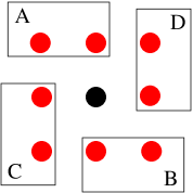
Jamming percolation, a new class of two-dimensional correlated percolation models inspired by kinetically constrained models, was introduced by Toninelli, Biroli, and Fisher Knight ; Knight.longer ; Spiral.longer . These models consist of the following occupation constraints: a site can remain occupied only if there exists at least one occupied site in set A and one occupied site in set B, or one occupied site in set C and one occupied site in set D. All sets are disjoint from each other and contain two sites. See Fig. 1 for the sets in a jamming percolation model called the spiral model. Jamming percolation models exhibit discontinuous phase transitions with a crossover length scale that diverges faster than any power law. It has been recently demonstrated that this behaviour prevails when more than four disjoint sets are introduced JammingPerc.JSP . While there are rigorous results for some models in this class, it is unknown how generic this transition is and whether or not there are other unusual, or atypical, phase transitions of correlated percolation.

Figure 1: Sets for the spiral model.

Here, we present a class of correlated percolation models denoted as force-balance percolation models. Force-balance percolation was originally introduced in Ref. SLC as a toy model for the jamming transition in finite dimensions. The jamming transition is a transition from a liquid-like to an amorphous solid-like state as some particular control parameter, such as the packing density, is varied. Examples of potentially related jamming systems are glass-forming liquids, colloidal suspensions, foams, emulsions, and granular matter Liu.Nagel.PointJ . Despite decades of study of the glass-forming liquids in particular, however, it is even unclear whether these transitions are true thermodynamic transitions or merely examples of kinetic arrest glass.review .

There has been some recent activity focusing on a zero-temperature jamming transition in a system of repulsive soft spheres as the packing density is increased. Numerical simulations by O’Hern, et al. considered repulsive soft particles in two and three dimensions OHern.simulations ; Langer . For small packing fraction $\phi$, the particles easily arrange themselves so as not to overlap with any other particle, and the total potential energy thus vanishes. As $\phi$ is increased, there is a particular value of $\phi_{c}$ (Point J) above which the particles can no longer avoid each other and the total potential energy becomes nonzero. The system jams in that it develops nonzero static bulk and shear moduli above $\phi_{c}$. The average coordination number (the average number of overlapping neighbors per particle) jumps from $Z=0$ to $Z=Z_{c}$ at Point J, and then rises with increasing packing fraction $\phi$ as $Z-Z_{c}\sim(\phi-\phi_{c})^{\beta}$, where $\beta=0.5$. This behaviour was recently observed in a two-dimensional systems of glass beads glass.beads.expt . Furthermore, as $\phi$ approaches $\phi_{c}$ from above, the singular part of the shear modulus vanishes with the exponent $\gamma=0.5$; more recent simulations also find that there is a length scale that diverges with an exponent $\nu=0.25$ PointJ.more.sims . So the transition at Point J appears to have characteristics of both first-order and second-order phase transitions: at the transition, $Z$ is discontinuous, but there are nontrivial power laws.

To understand this somewhat unusual transition, an analogy to $k$-core/bootstrap percolation was made in Ref. SLC . The scalar aspect of the principle of local mechanical stability, where particles need $d+1$ contacts, maps to a requirement of $k$ occupied neighbors. Surprising agreement was found between the mean-field $k$-core percolation exponents and the repulsive soft sphere simulations. We note that the two- and three- dimensional simulations observed the same exponents, suggesting a possible critical dimension of two since logarithmic corrections would be difficult to determine wyart .

While there is agreement between the mean field $k$-core exponents and the low-dimensional repulsive soft sphere exponents, $k$-core in finite-dimensional spaces does not appear to have such agreement. Such systems seem to fall into one of two classes: the transition is either continuous and in the same universality class as normal percolation, or it does not occur until $p_{c}=1$. In the first class, systems that allow finite clusters all exhibit continuous transitions chavez ; medeiros . In the second class, large voids are very likely to grow, and in the infinite system limit, with probability one there will be at least one void that will grow to empty the entire system kcore.odd.old.1 ; kcore.rigorous.1 . This prevents $k$-core percolation for any $p<1$. Unfortunately, neither category of $k$-core percolation describes the nontrivial discontinuous transition observed in the finite-dimensional simulations and experiments of jamming.

In an effort to try to capture the behaviour of jamming in finite dimensions, force-balance percolation was introduced in Ref. SLC . In this model, the $k$-core constraint is retained, but the vectorial constraints of the principle of local mechanical stability are mimicked by creating culling rules that take into account where the neighboring particles are located. Loosely speaking, if there is a neighboring contact to one side of the particle, there must be at least one neighboring contact on the other side of the particle to allow for force balance.

We must emphasize the force-balance percolation is a model with no explicit forces. We look only at connectivity, in contrast to models such as rigidity percolation where repulsive and attractive forces are defined on, say, a lattice of springs rp1 ; rp2 ; rigidity.percolation.3 ; rigidity.percolation.4 . However, the nature and possible universality of the rigidity percolation transition is still up for debate, despite decades of study. Since force-balance percolation is a much simpler model there is ultimately a better chance of analyzing it beyond numerics.

Here, we explore several versions of force-balance percolation, both rigorously and numerically, to begin to answer the following questions:

(0) Is there a force-balance percolation transition?
(1) If there is indeed a transition, what are its properties? Is it continuous?
(2) How generic is the transition among the various force-balance models?
(3) Is there a link between force-balance percolation and jamming percolation? Are they in the same universality class?

The paper is organized as follows. In section II we review the force-balance percolation model introduced in Ref. SLC , and introduce two related models. We present in section III a rigorous proof that the thermodynamic $p_{c}$ is less than unity for at least two of these models. Earlier work on $k$-core percolation misinterpreted numerical results, finding transitions in novel universality classes, with $p_{c}<1$ kcore.odd.old.1 ; kcore.odd.old.2 ; kcore.odd.old.3 , when in fact the models studied had $p_{c}=1$ kcore.rigorous.1 ; kcore.rigorous.2 ; kcore.rigorous.3 ; our proof renders our subsequent interpretation of the numerical data presented in section IV on sounder footing. Finally, we close in section V with a summary of our findings and discuss their implications.

II Models

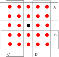
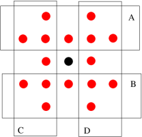
For the first force-balance percolation model, we begin with a two-dimensional square lattice. Each site neighbors all sites except itself within a 5x5 square—each site therefore has 24 nearest neighbors. (For a 3x3 square, with the following rules, $p_{c}=1$). Since we are in two dimensions, we impose a 3-core constraint. However, we also impose the force-balance constraint, which is the following: there must be at least one occupied neighbor in set A, which in turn calls for at least one occupied neighbor in set B, and there must be at least one occupied neighbor in set C, which in turn calls for at least one occupied neighbor in set D. The four sets A, B, C, and D, are defined in Fig. 2. The force-balance constraint can be succinctly stated as: (A and B) and (C and D), where each letter X is short for “at least one occupied site in set X”. Note that the force-balance constraint is defined in such a way such that vertical and/or horizontal lines of occupied particles are, by themselves, not stable. Fig. 3a demonstrates an allowed configuration and Fig. 3b demonstrates a prohibited configuration.

To enforce the force-balance and $k$-core constraints, we initially occupy sites on the lattice with independent occupation probabilities $p$, and then repeatedly remove occupied sites that violate either the $k$-core or force-balance constraints, until all remaining occupied sites are stable. Note that $p$ is the occupation density before culling, and generically differs from the final occupation density.

Figure 2: Force-balance model on the 2$d$ square lattice with 24 nearest neighbors.

Figure 3: Black sites denote occupied sites, and red sites denote unoccupied sites. (a) Allowed configuration. (b) Forbidden configuration. While the number of occupied nearest neighbors is greater than three, the force-balance condition is violated.

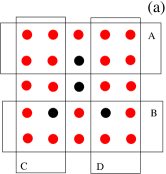
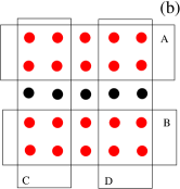
The model is abelian. In other words, the final configuration after the culling process is independent of the order in which sites are culled. It can be done in parallel, or in series, or some combination thereof. One can define another force-balance-like model that allows for horizontal and vertical lines of occupied neighbors. However, such a model would be nonabelian. Nonabliean models are less desirable, because in such models the final results depend on the order in which sites are culled. In our work, the culling procedure is merely an algorithm to achieve the force-balance percolation configuration.

To determine whether or not the behaviour observed in the original force-balance model is generic, we define two additional abelian models. Our second model is defined on the square lattice, with 16 nearest neighbors, and quadrants as defined in Fig. 4. Again, $k=3$ and the force-balance constraint is the same as above: (A and B) and (C and D). This model is obviously similar to the first one, though the ratio of $k$ to $Z_{max}$ is different.

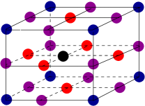
The third model is a three-dimensional model with 26 nearest neighbors and six regions, color-coded in Fig. 5. Each of the six regions consists of a $3\times 3$ square on a face of the $3\times 3\times 3$ cube centered on the site whose stability is being analyzed. For this model, we impose a 4-core constraint (since $d=3$), and the force-balance condition requires an ocupied site in each of the six regions.

For comparison, along with numerical simulations of these three models, we also performed simulations on the spiral model. This model was introduced by Toninelli, et al. TBF.response ; Spiral.longer , and they have proved that it undergoes a jamming transition, and obtained rigorous results about the properties of the transition Spiral.longer .

Figure 4: A second force-balance model on the $2d$ square lattice with 16 nearest neighbors.

Figure 5: Force-balance model on the $3d$ cubic lattice with 26 nearest neighbors. A red site participates in only one of the six sets, a purple site in two of the six sets, and a blue site in three of the six sets.

III Rigorous Results

III.1 Proof that $p_{c}<1$ in the $2d$ force-balance models

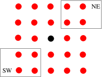
To prove that $p_{c}<1$ for the initial force-balance model on the square lattice, we will demonstrate that $p_{c}<1$ for a more heavily constrained model with the same 24 nearest neighbors. In particular, we require (1) $k=6$, (2) at least one occupied neighbor in the 4-site region to the northeast, and (3) at least one occupied neighbor in the 4-site region to the southwest. See Fig. 6 for the two regions. Since any sites stable under these conditions are automatically stable in the force-balance model, if $p_{c}<1$ for the $k=6$ NE-SW model, then also $p_{c}<1$ for the force-balance model.

Figure 6: $k=6$ NE-SW model.

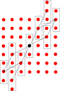
Next, we prove that the origin has a non-zero probability of participating in an infinite cluster for the $k=6$ NE-SW model. We divide the lattice into clusters of three sites, as shown in Fig. 7. Certain clusters are defined as adjacent, and connected by directed lines in Fig. 7. Sites not grouped in 3-clusters play no role in the proof, and can be ignored. Now, suppose that $p>(p_{c}^{DP})^{1/3}$, where $p_{c}^{DP}$ is the critical probability for two-dimensional directed percolation. Then each 3-cluster is occupied with probability $p^{3}>p^{DP}_{c}$. The directed lines in Fig. 6 are isomorphic to two-dimensional percolation. Thus, the probability of the origin participating in an infinite chain of 3-clusters to the northeast is nonzero, provided the 3-cluster at the origin is occupied. Similarly, the probability of the origin participating in an infinite chain of 3-clusters to the southwest is also nonzero. Looking only at the infinite chain of 3-clusters, it is straightforward to check that every site in it is stable under the culling rules. To see this, observe that each 3-cluster in the infinite path has only four possible configurations of adjacent 3-clusters, shown in Fig. 8. For all four configurations, all sites in the central 3-cluster are stable under the $k=6$, NE-SW stability condition. Therefore, $p_{c}<(p_{c}^{DP})^{1/3}<1$. This bound holds for $k\leq 6$ for the force-balance model, since the force-balance constraints are a subset of the constraints in the NE-SW model.

A similar proof holds for the 16 nearest-neighbor force-balance model. For this model, one can construct 2-clusters to obtain a proof that for $k\leq 4$ we have $p_{c}\leq(p_{c}^{DP})^{1/2}$.

We note that a simple lower bound for $p_{c}$ for both models is the $p_{c}$ of the corresponding uncorrelated percolation models (i.e. the $p_{c}$ of the model without culling).

Figure 7: Adjacent clusters of 3 sites in the NE-SW model.

Figure 8: Local configurations of 3-clusters in the NE-SW model.

Regarding the three-dimensional model, as was shown in Ref. JammingPerc.JSP , for three-dimensional versions of the jamming percolation models, percolating structures along one direction can cross without having sites in common. This prevents an obvious mapping to directed percolation. We have therefore not obtained a rigorous bound for $p_{c}$ in the three-dimensional model.

III.2 Nature of the transition?

While it can be shown that $p_{c}<1$ for the two-dimensional models, there is no proof as to whether the transition is continuous or discontinuous. For the two-dimensional jamming percolation models, there exists a rigorous argument for a discontinuous transition assuming a conjecture regarding directed percolation Knight ; Spiral.longer . The argument relies on having two independent directed percolation processes arising from the disjoint pairs of sets, each containing two sites. The jamming percolation transition can then be shown to occur at the directed percolation transition point. In the force-balance models considered here, the sets are composed of more than two sites, and are not disjoint. The critical occupation probability thus cannot be easily identified. This means that it is not obvious how to construct a rigorous argument along the lines of the jamming percolation models.

However, we first argue that the alteration of some properties of the jamming percolation models to make them look more like force-balance percolation should not change the nature of the jamming percolation transition. For example, the property of having two sites per set in the jamming percolation models can be extended to having more sites per set by investigating other lattice models with more nearest neighbors, but belonging to the same universality class as directed percolation. Surely, there exist other directed percolation processes with more than two neighbors per site.

On the other hand, the force-balance rules can be modified to be more like the jamming percolation models, where the “and” between overlapping sets is equivalent to “or” between various pairs or triplets of smaller disjoint sets. See Fig. 9. While the occupation of pairs of disjoint sets are the same as in the jamming percolation case (excluding the $k$-core constraint where more than one site in the set must be occupied for the pairs), the occupation of triplets are more stringent. It remains to be seen whether or not a rigorous argument can be constructed for force-balance percolation.

Figure 9: The force-balance rules can be implemented with (A’ and C’) or (D’ and B’) or (E’ and B’ and C’) or (F’ and C’ and D’) or (G’ and A’ and B’) or (H’ and A’ and D’) or (A’ and G’ and H’) or (B’ and E’ and G’) or (C’ and E’ and F’) or (D’ and F’ and H’) or (E’ and F’ and G’ and H’).

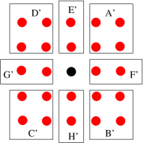
Given these arguments, the transition for the force balance percolation models may in fact behave similarly to the jamming percolation models and so we expect the transition in the force-balance case to be discontinuous as well. We will numerically test this hypothesis as well as others in the upcoming section.

IV Numerical results

IV.1 24 NN model

IV.1.1 Culling dynamics

We begin our numerical simulations of the 24 NN (nearest neighbor) force-balance model by looking at the dynamics of the culling process. The lattice is size $L$ by $L$. We surround it with a boundary of fully occupied sites, two layers thick, which are never culled. We denote this as wired boundary conditions. Then, at each timestep, we simultaneously cull every unstable site. We repeat this until all remaining sites are stable and record the culling time.

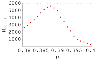
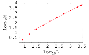
For any given system size, the mean culling time as a function of the initial occupation density peaks for some density—a sample curve for $L=2896$ is shown in Figure 10. The density at which the curve peaks provides one possible definition of the critical density. The size of the peak is denoted by $M$, the maximum number of average culls. $M$ grows with $L$. We plot $M$ vs. $L$ on a log-log scale in Figure 11. The results are well fit by a power law, although there is visible overall curvature. A best fit for $L\geq 32$ gives $M\propto L^{\alpha}$, with $\alpha=1.226\pm 0.027$, which is suggestively close to $5/4$.

We note that $5/4$ is the dynamical exponent for avalanches in the sandpile model ASM.5over4.numerics . Priezzhev has given an analytical argument that the dynamics exponent for the sandpile model should be exactly $5/4$ ASM.5over4.Priezzhev . More generally, Pietronero, et al. ASM.5over4.numerics have given a renormalization group argument that the avalanche exponent should be the same for a wide class of “sandpile-like” models ASM.5over4.RG . They obtain an approximate exponent of $1.253\approx 5/4$. “Sandpile-like” models are those in which energy is dissipated, so that instabilities propagate from site to site. A similar process may be responsible for the exponent of $5/4$ seen in our models here: culling at a site may be analogous to toppling at a critical point of a sandpile-like model, in the sense that the culling of one site triggers adjacent cullings that can propagate long distances.

Figure 10: Mean culling time as a function of initial occupation density for the 24 NN model, $L=2896$.

Figure 11: Peak of the mean culling time as a function of $L$ for the $24$ NN model. The best fit has a slope of $1.226\pm 0.027$. The same data is also plotted for the spiral model.

IV.1.2 Force-balance avalanches

Farrow, et al.  Duxbury studied the dynamics of culling in $k$-core percolation on various lattices by looking at avalanches. More precisely, the culling process is iterated until a stable $k$-core configuration is obtained. Then, a random site in the stable $k$-core is removed. It triggers the removal of other sites until the $k$-core stabilizes once more. The number of sites removed during this removal is the culling avalanche size. The process is repeated until the lattice is completely empty. In cases where $p_{c}=1$ and the stability rules allow no finite clusters, a power-law distribution of culling avalanche sizes was found. For these cases, the system goes from being unoccupied for $p_{c}<1$, to being fully occupied at $p_{c}=1$. Since all sites must be eventually be removed below $p_{c}=1$ and no finite clusters are allowed, the culling avalanches should become spatially long-ranged near $p_{c}=1$. This result is to be contrasted with $k$-core cases with finite $k$-core clusters. There, no power law distribution of culling avalanche sizes was found Duxbury .

In the force-balance model, there are no finite force-balance clusters, so the culling avalanches should be spatially long-ranged near the transition. Whether or not there should be a broad distribution of sizes is not clear a priori. Given the sandpile-like behavior detected in the mean culling time required to obtain a force-balance cluster, one may expect to find a broad distribution as is found in sandpile models. However, if the force-balance percolation transition is discontinuous one would expect a well-defined avalanche size for those systems whose redundant sites have already been removed.

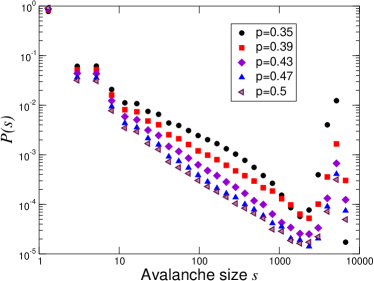
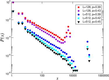
Numerically, we calculate the probability of having a culling avalanche size $s$, $P(s)$ in the presence of periodic boundary conditions. See Fig. 12. The probability is broad near and above the transition for intermediate avalanche sizes. On a log-log plot, the slope of $P(s)$ for the broadly distributed intermediate-sized avalanches depends somewhat on $p$ and on $L$. More careful study is needed to determine whether or not these avalanche sizes are consistent with the measured $-1.253$ for sandpile models ASM.5over4.RG . It is of note that for $p=0.45$ and $L=512$, for example, the slope is approximately $-1.3$.

As opposed to quantitative analysis of the intermediate-sized avalanches, we are more interested in first determining the qualitative nature of the curves. As opposed to a purely broad distribution, there is a prominent peak at the tail of the distribution. These well-defined avalanche sizes correspond the last occuring avalanches when the lattice ultimately empties out. These correspond to the marginal infinite cluster. The peak persists as $p$ is decreased towards the $p_{c}$ indicated from the position of the maximum in the mean culling times, suggesting a discontinuous transition for the onset of the infinite cluster. This behaviour is retained in the larger systems with the peak becoming more separated from the broad part of the distribution. See Fig.  13.

Figure 12: Log-log plot of $P(s)$ for $L=128$ using periodic boundary conditions.

Figure 13: Log-log plot of $P(s)$ for $L=128$ and $L=512$ for comparison. The $L=512$ curves have been shifted downward by a factor of 0.1.

IV.1.3 Spanning cluster

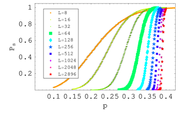
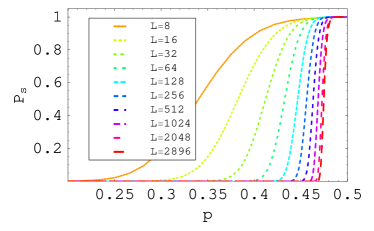
We next look at $P_{s}$, the probability of spanning. We define this, for wired boundary conditions, as the probability that the largest cluster connects either the top and bottom sides, or the right and left sides; for this definition, sites are defined as connected if one is within the 24 site neighborhood of the other (see Fig. 2). Fig. 14 depicts $P_{s}$ for the 24 NN model with wired boundary conditions.

Fig. 15 shows the same curves, but for periodic boundary conditions. For periodic boundary conditions, it is impossible to have any occupied sites without having a spanning cluster, so to check if we have a spanning cluster, we just need to check that at least one site is occupied.

Figure 14: The probability of spanning for wired boundary conditions in the $24$ NN model.

Figure 15: The probability of spanning for periodic boundary conditions in the $24$ NN model. Error bars are too small to be seen.

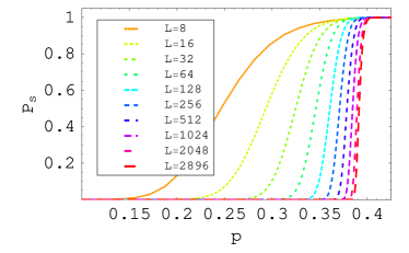
For periodic boundary conditions, the $P_{s}$ curves can be generated quickly by a simple modification of the Newman-Ziff algorithm Newman.Ziff . For uncorrelated percolation, the Newman-Ziff algorithm passes once through every possible density, in increasing order, by adding occupied sites in random order, and updating the connectivity with the Hoshen-Kopelman algorithm Hoshen.Kopelmann . This allows for efficient generation of $P_{s}$ for every occupation density. This method is not available to us for the force-balance model with wired boundary conditions, because there sites are added by increasing the density, but also removed by culling. This prevents a single pass through all densities from being done in time $\mathcal{O}(L^{2}\ln L)$. (The Hoshen-Kopelmann algorithm does not allow cluster identifications to be rapidly updated after removal of sites.) However, with periodic boundary conditions in a force-balance model, we do not need to run the Hoshen-Kopelman algorithm. We can instead start from a fully occupied lattice, and remove sites until the culling condition causes an empty lattice. This allows the calculation of $P_{s}$ at every density in time $\mathcal{O}(L^{2})$.

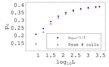
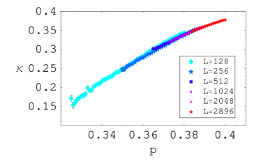
From Figs. 14 and 15, we can define the critical probability for a specified system size, $p_{c}(L)$, as the initial occupation density that gives $P_{s}=1/2$. This definition differs from that based on the peak of the mean culling time, given in subsection IV.1.1. However, as shown in figure 16, the two definitions have the same qualitative dependence on $L$, and approach each other for large system sizes.

Figure 16: $p_{c}(L)$ for the $24$ NN model, using two definitions of the critical point: (1) the density at which $P_{s}=1/2$, and (2) the density at which the mean culling time peaks.

Given $p_{c}(L)$ we can extract the thermodynamic critical point, $p_{c}(L=\infty)$, if given the functional dependence of $p_{c}(L)$ on $L$. However, it is unclear what functional dependence to fit to. It was assumed in Ref. SLC that $|p_{c}(L=\infty)-p_{c}(L)|\propto L^{-1/\nu}$, where $\nu$ is an exponent characterizing the divergence of the length scale. With this functional form, $\nu$ can be detected by varying $p_{c}(\infty)$ until a log-log plot gives a straight line. However, such a procedure is not a check of the functional form, since we are allowed to choose $p_{c}(\infty)$.

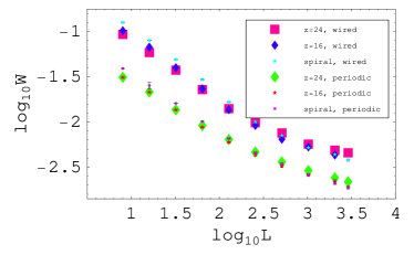
A check of the functional form can be done by looking at the width $W$ of the transition, which we define to be the difference between the occupation probabilities that yield $P_{s}=1/4$ and $P_{s}=3/4$. The width as a function of $L$ is shown in figure 17 for both wired and periodic boundary conditions. The same renormalization group formalism that implies $\mid p_{c}(L=\infty)-p_{c}(L)\mid\propto L^{-1/\nu}$ also implies $W\propto L^{-1/\nu}$. However, Fig. 17 shows clear deviations from this power law form. This trend was starting to emerge in Ref. SLC , though it was masked by the large error bars for the larger systems. In other words, the fit to the above assumption in Ref. SLC was premature.

Figure 17: The widths for the 24NN model with both wired and periodic boundary condition, on a log-log plot. Both boundary conditions show clear deviations from power laws at large system sizes.

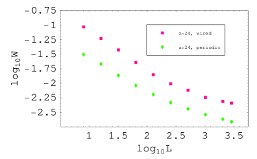
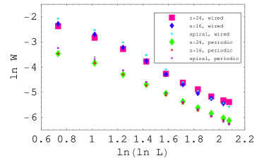
Based on our above heuristic arguments for a connection between force-balance percolation and jamming percolation, we instead fit to the form for a diverging crossover length scale found by Toninelli, et al. TBF.response ; Spiral.longer (TBF) for the spiral model. Approaching the transition from below, TBF identified a crossover length $\Sigma$, such that systems of size smaller than $\Sigma$ are likely to have a spanning cluster, while those of size greater than $\Sigma$ are exponentially unlikely to have a spanning cluster. TBF proved that $\Sigma$ diverges at the transition faster than any power law. In Ref. Knight , TBF argued that the upper and lower bounds scaled similarly, finding $\Sigma\sim\exp(-C(p-p_{c})^{-\mu})$, where $\mu=(1-\frac{1}{z})\nu_{||}\cong 0.64$. (Both $\frac{1}{z}\cong 0.63$ and $\nu_{||}\cong 1.73$ are from directed percolation DP .) Based on the TBF formula, we propose that $W\propto(\ln(L))^{-1/\mu}$. The widths are replotted with the appropriate scales for this fit in Figure 18, and while the curves still have deviations from perfect straight line behavior, the agreement is significantly better than for $W\propto L^{-1/\nu}$. From the width data, for wired boundary conditions, we extract $\mu=0.39\pm 0.01$; for periodic boundary conditions, $\mu=0.45\pm 0.02$. The stated error bar is purely statistical and does not take into account systematic effects that occur given the small range of system sizes, so one cannot necessarily rule out a link with overlapping directed percolation processes. We also note that in Ref. Knight , TBF stated that their numerical data was consistent with $\mu\cong 0.64$ given the large systematic error bars.

Figure 18: The widths for the 24NN model with both wired and periodic boundary condition, using a fitting form motivated by the TBF results.

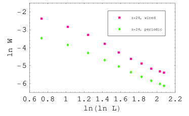
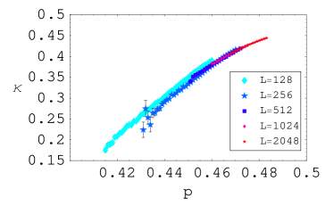
Now, if there is only one diverging lengthscale, then it can be argued that $|p_{c}(L)-p_{c}(\infty)|$ should be proportional to $W$. So we choose the TBF fitting form and choose $p_{c}(\infty)$ to minimize $\chi^{2}$ for the best linear fit of $\ln(p_{c}(\infty)-p_{c}(L))$ vs. $\ln(\ln L)$, for $L\geq 32$. The optimal fit, shown in figure 19, is obtained for $p_{c}(\infty)=0.414\pm 0.008$ for wired boundary conditions. (The error bar is obtained by testing which values of $p_{c}(\infty)$ result in visibly noticeable curvature in the plot.) For periodic boundary conditions, we obtain $p_{c}(\infty)=0.425\pm 0.005$. The straight line obtained in figure 19 does not make clear whether the TBF form is correct for our model, given that we have the freedom to choose $p_{c}(\infty)$ in making the fit. From the fit with wired boundary conditions we obtain $\mu=0.51\pm 0.09$. Again, this result is to be compared with TBF’s result of $\mu=0.64$.

From the two different results for $\mu$, it appears that $W$ and $|p_{c}(L=\infty)-p_{c}(L)|$ do not scale in the same way. There are two possible, but incompatible, explanations for the difference in the results for $\mu$. One possibility is that the scaling of $W$ and $|p_{c}(L=\infty)-p_{c}(L)|$ is in fact the same in the thermodynamic limit, but that we obtain differing $\mu$’s for the finite system sizes studied due to the slow approach to the thermodynamic limit. This would be reminiscent of the extremely large finite-size effects seen in analogous systems, such as $k$-core percolation, the Kob-Andersen model, and glassy dynamics. Numerically, this possibility is quite reasonable, given that the TBF formula for the growing length scale has an extra power law factor in front. A second possible explanation is that $W$ and $|p_{c}(L=\infty)-p_{c}(L)|$ in fact scale differently. This would be possible if there are are two diverging length scales, rather than one; this would change the standard picture of a renormalization group fixed point controlled by a single parameter, so that $W$ and $|p_{c}(L=\infty)-p_{c}(L)|$ would no longer be forced to scale in the same manner. There are certainly two diverging lengthscales in mean field $k$-core percolation—one associated with those in the infinite cluster and one associated with sites that get removed in response to one random site being removed.

Figure 19: Fitting of $p_{c}(L)$ as a function of $L$ using the TBF fitting form, for the $24$ NN force-balance model with wired boundary conditions. We obtain the best fit with $p_{c}(\infty)=0.414\pm 0.008$.

IV.1.4 Order parameter

We also investigate the order parameter, $\kappa$, the fraction of sites in the infinite force-balance cluster. This is obtained for a given system size and initial occupation density by generating configurations, keeping only those configurations in which the largest cluster is spanning, and then finding the average fraction of sites in the largest cluster for those configurations. Plots are shown for $L\geq 128$ in figure 20. The curves lie on top of each other for large $L$, differing only in the minimum value of $p$ needed for the numerical simulations to have a reasonable chance of obtaining occupied sites after culling.

The minimum value of $\kappa$ is increasing, rather than decreasing, with system size. We therefore assume that there is a jump in the order parameter at the transition, denoted by $\kappa_{c}$. In other words, in the thermodynamic limit, as soon as there is a spanning cluster, it occupies a finite fraction of the system.

From Fig. 20, and the already-obtained result of $p_{c}=0.414\pm 0.008$, we estimate the thermodynamic $\kappa_{c}$ to be $\kappa_{c}=0.399\pm 0.011$. Furthermore, for each individual curve it appears that just above the transition, $\kappa$ increases linearly with $p$, suggesting that the order parameter exponent is $\beta=1$. This result is to contrasted with the mean field $k$-core percolation results and the repulsive soft sphere simulations, where $\beta=1/2$.

Figure 20: Order parameter for the $24$ NN model using wired boundary conditions.

IV.1.5 Correlation function

We next look at correlation functions for this model, now using only periodic boundary conditions. For these simulations, for a given system of size $L$ and density $p$, we generate states with exactly $pL^{2}$ occupied sites (rather than occupying sites independently). We only keep configurations that were nonempty after culling, and in each of these, keep only the largest cluster (this cluster was automatically spanning, since we use periodic boundary conditions). We then calculate the correlation function $C(i)$—the probability that sites a distance $i$ apart are both occupied, minus an asymptotic constant, to be discussed shortly. Moreover, we calculate correlations at all angles (i.e. not merely horizontal and vertical correlations).

With uncorrelated percolation, it is easy to quickly produce precise plots of the correlation function over several decades of distance, and confirm that the correlation function has a power law form at the critical point. However, correlations in the force-balance model have significantly greater sources of uncertainty.

When we generate samples for uncorrelated percolation, each site occupation is independent, so the correlation function calculated for $C(i)$ is largely (although not entirely) independent of that for $C(j)$ with $j\neq i$. So for uncorrelated percolation, when we look at different pairs of points in a single sample, we get somewhat independent estimates of the correlation function for a range of distances. That is, we quickly generate lots of independent data for the curve $C(i)$. However, for correlated percolation models where there are no finite clusters, the results for $C(i)$ and $C(j)$, for $j\neq i$, are are highly correlated for a given sample, even for widely separated $i$ and $j$.

For a given amount of computer running time, the error bars in the correlation function are thus substantially larger than for uncorrelated percolation, and because they are correlated, it is difficult to reliably extract the asymptotic value of $C(i)$. This is important because to get $C(i)$, we need to subtract off the probability that two distant sites ($i\to\infty$) are occupied in the infinite system limit ($L\to\infty$) after culling. For our models, we do not know the infinite system occupation probability after culling. (For uncorrelated percolation, it is trivially identical to the initial occupation probability, as there is no culling). The most straightforward solution is to subtract off the asymptotic value of $C(i)$, since we know that the connected correlation function should approach $0$ as $i\to\infty$. However, because the error bars at different $i$ are correlated, there are also large error bars in the asymptotic value of $C(i)$. The functional form of $C(i)$ is highly sensitive to the constant subtracted off—over a limited distance range, a power law and an exponential can look very similar if the asymptotic value is shifted slightly. This means that that it is difficult to reliably determine the form of the correlation function. The correlation length,

$$\xi^{2}=\frac{\sum_{i}i^{2}C(i)}{\sum_{i}C(i)}\ ,$$ (1)

is also very sensitive to a small shift in $C(i)$.

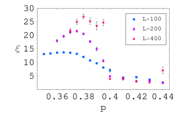
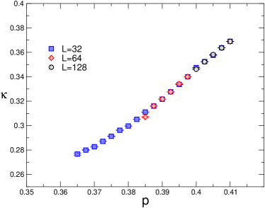
The end result is that it is difficult to get accurate results for large system sizes, and we have limited our simulations of correlation functions to $L=100$, $L=200$ and $L=400$. The correlation length as a function of initial occupation density is shown for these three system sizes in figure 21. For densities $\rho>0.4$, the correlations are clearly short-ranged, and are independent of the system size. For lower densities, the correlation length grows with $L$. The curve for $L=200$ has a clear peak at $p\approx 0.375$; the $L=400$ data appears to have a peak at a larger $L$, although the largish error bars make its location unclear. Thus, the data is somewhat suggestive of a lengthscale that grows with system size.

The position of the peak gives yet another plausible measurement for $p_{c}(L)$. If we compare the $p_{c}(L)$ defined from the probability of spanning for $L=200$, $p_{c}(L)=0.3671\pm 0.0007$, which is lower than the estimated $p_{c}(L)$ from correlation length data. However, this discrepancy should vanish in the infinite system limit. Since the position of the peak is not so clear for $L=400$ it is more difficult to discern the trend.

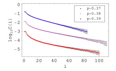
Because of the limited system sizes studied, it is somewhat difficult to determine with confidence whether the correlation functions have power law or exponential forms. The correlations are very short-ranged ($\xi<5$) for $p\geq 0.4$, indicating that the correlations are probably exponential (or a very steep power law). At lower densities, for most system sizes and densities, the correlation function is exponentially decaying at long distances; for example, see figure 22, showing the correlation functions for $L=400$ and $p=0.37$, $0.38$, and $0.39$. One exception to the generally observed exponentialy behavior is te $L=200$ correlation function for $p=0.395$, which appears somewhat power-law-like, as shown in figure 23. The density of $p=0.395$ differs slightly from the peak in the plot of $\xi$ for $L=200$ in figure 21. For the $L=400$ system, the power-law-like trend of the correlation function near the peak density is not as prominent and the correlation functions appear more exponential.

Figure 21: Correlation lengths for the $24$ NN force-balance model as a function of $p$, for $L=100$ and $L=200$.

Figure 22: Correlation function for $L=400$, for the $24$ NN force-balance model, at $p=0.37$, $p=0.38$, and $p=0.39$. For clarity, the $p=0.37$ correlation function has been shifted up by 1.0, and the $p=0.39$ correlation function has been shifted down by 1.0.

.

Figure 23: Correlation function for $L=200$, $p=0.395$, for the $24$ NN force-balance model. The best fit line has a slope of $-1.76\pm 0.03$.

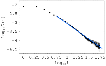
These results should be compared with those of Parisi and Rizzo for k-core percolation in four dimensions Parisi . While they found that $\xi$ grew with decreasing $\rho$, they never obtained correlation lengths greater than 10. So they also found no power law correlations. They argue that the 4-core transition in four dimensions is an ordinary discontinuous transition with no diverging lengthscales. We note that their systems had finite stable clusters and so may have different properties than the systems considered in this paper. (The fact that their systems had finite stable clusters also presumably means that they had smaller numerical correlations between $C(i)$ and $C(j)$ for $\mid i-j\mid$ large, allowing them to determine correlation functions for larger systems than here.)

IV.2 16 NN Model and Spiral Model

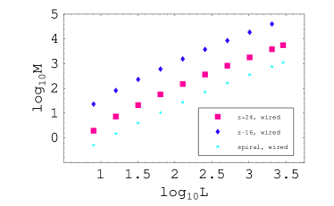
Now we present results for the 16 nearest neighbor force-balance model and spiral model. We begin with the mean culling time. The plot of the mean peak culling time as a function of $L$ shows a similar $5/4$ exponent as was measured for the 24NN model, $\alpha=1.240\pm 0.025$. In fact, all three two-dimensional models—the 24NN model, the 16NN model and the spiral model—are in quantitative agreement with another. We find $\alpha=1.246\pm 0.027$ for the spiral model. These results suggest that similar processes underlie the culling in all three two-dimensional models. See Fig. 24.

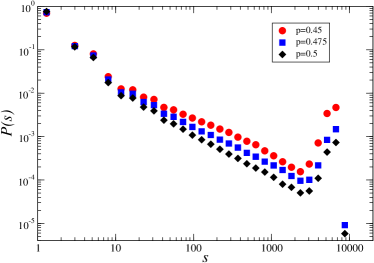
The probability of having a force-balance avalanche of size $s$, $P(s)$, for the 16 NN model shows similar trends to the 24 NN model with a broad distribution of intermediate sizes and a prominent peak for the largest sizes. See Fig. 25. The spiral model exhibits the same qualitative behaviour as well.

Fig. 26 shows the probability of spanning for periodic boundary conditions. From this data we extract the width of the transition as a function of $L$, as depicted in Fig. 27. We plot both periodic and wired boundary conditions on a log-log scale to demonstrate the significant deivations from a power-law growing crossover length. We also plot the same data for the 24NN and spiral models for comparison. As with the 24NN model, the fitting form is clearly not a power law in $L$. Figure 28 shows the widths using the fitting form motivated by the TBF result. For the 16NN model, one can extract $\mu=0.35\pm 0.01$ for wired boundary conditions and $\mu=0.42\pm 0.03$ for periodic boundary conditions.

In Fig. 29, similarly to Fig. 19, we choose $p_{c}(\infty)$ so that $p_{c}(\infty)-p_{c}(L)$ as a function of $L$ is well fit by the TBF functional form. We obtain the best fit for $p_{c}(\infty)=0.497\pm 0.007$ for wired boundary conditions, which gives $\mu=0.47\pm 0.07$. For periodic boundary conditions, $p_{c}(\infty)=0.502\pm 0.010$ and $\mu=0.70\pm 0.15$. Once again, there is a discrepancy between the $\mu$ extracted from the width data and the $\mu$ extracted from the one-parameter fit.

A similar fit (not shown) for the spiral model finds $p_{c}(\infty)=0.690\pm 0.008$, and $\mu=0.49\pm 0.08$ for wired boundary conditions. For the spiral model, Toninelli, et al. TBF.response ; Spiral.longer have proven that $p_{c}(\infty)$ is the same as for direct percolation, $p_{c}(\infty)\cong 0.705$, and found $\mu=0.64$. Our numerical results for $p_{c}(\infty)$ and $\mu$ are both within two error bars from their exact result, and a plot of $\ln(p_{c}(\infty)-p_{c}(L))$ versus $\ln(\ln L)$ for the exact result of $p_{c}(\infty)\cong 0.705$ shows noticeable curvature. Also, the $\mu$ extracted from the width data for wired boundary conditions is $\mu=0.32\pm 0.01$ and $\mu=0.38\pm 0.02$ for periodic boundary conditions.

Finally, Fig. 30 shows the order parameter $\kappa$ as a function of $p$ for various system sizes for the 16NN model. As in the 24 NN model, the jump in $\kappa$ increases with increasing system size suggesting that the transition is discontinuous. It also appears that $\beta=1$ just above the transition for each individual curve (though there is some overall curvature for the set of curves).

Figure 24: Peak of the mean culling time as a function of $L$ for the all three models. For the 16NN model, the best fit has a slope of $1.240\pm 0.025$. For the spiral model, the best fit has a slope of $1.246\pm 0.027$. Wired boundary conditions are used.

Figure 25: Log-log plot of $P(s)$ for the 16 NN model with $L=128$ in the presence of periodic boundary conditions.

Figure 26: The probability of spanning for periodic boundary conditions for the $16$ NN force-balance model. Error bars are too small to be seen.

Figure 27: The widths for all three models with both wired and periodic boundary condition, on a log-log plot. All curves show clear deviations from power laws at large system sizes.

Figure 28: The widths for all three models with both wired and periodic boundary condition assuming the TBF form.

Figure 29: Fitting of $p_{c}(L)$ as a function of $L$ using the TBF fitting form, for the $16$ NN force-balance model with wired boundary conditions. We obtain the best fit with $p_{c}(\infty)=0.497\pm 0.007$.

Figure 30: Order parameter for the $16$ NN model using wired boundary conditions.

IV.3 Three-dimensional model

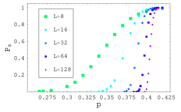
Our tests of the 26NN three-dimensional model are not as extensive as in the two-dimensional case, particularly because we have no proof that $p_{c}<1$ in this case and our system size range is limited. From the probability of spanning data using periodic boundary conditions, we have extracted $W$ and $p_{c}(L)$. See Fig. 31. Deteriming $p_{c}(\infty)$ with the TBF functional form yields $p_{c}(\infty)=0.433\pm 0.009<1$ (not shown). Moreover, for the one-parameter $p_{c}(\infty)$ fit, $\mu=0.75\pm 0.14$; from the width data, $\mu=0.37\pm 0.01$. In the three-dimensional case the discrepancy between the two values of $\mu$ for the same boundary condition is greater than the two-dimensional force-balance models, where larger system sizes can be explored. For this three-dimensional model, one may expect a double logarthim as opposed a single logarithm with potentially $\mu\cong 0.52$ using the values for three-dimensional directed percolation DP . Given the small range of data, however, it is difficult to discriminate between the two forms.

Finally, the three-dimensional transition appears to be discontinuous in the context of the onset of the infinite force-balance cluster, as in the two-dimensional cases, since the jump in the order parameter increases with increasing system size. See Fig. 32. Moreover, simulations of the probability of having a force-balance avalanche size $s$ shows the same trends as in Figs. 12 and 13.

Figure 31: Probability of having a spanning cluster in any of three directions, as a function of $p$, for different system sizes of length $L$, and periodic boundary conditions. This plot is for $k=4$ with force-balance on the cubic lattice with 26 nearest neighbors.

Figure 32: Order parameter plot for the three-dimensional model using periodic boundary conditions.

V Summary and Discussion

While uncorrelated percolation is very well understood, models of correlated percolation are much less so. We have presented rigorous and numerical results on several force-balance percolation models to help narrow the gap. On the rigorous side, we have proven that $p_{c}<1$ for the two-dimensional models. This result places our interpretation of the numerical data for the two-dimensional models on sounder footing. A rigorous argument that the force-balance percolation transition is discontinuous, at least in two dimensions, is more difficult than in the case of jamming percolation. In the jamming percolation models the underlying mechanism driving the transition is two disjoint, directed percolation processes. These two process scaffold upon one another such that the infinite cluster is bulky at the transition. The underlying mechanism driving the transition in the force-balance models is presumably the same as argued in Sec. IIIB. Models of newly-constructed directed percolation processes will be key in constructing a rigorous argument for discontinuity in the force-balance case.

Our numerical results for the force-balance avalanches and the onset of the infinite force-balance cluster for all three force-balance models strongly suggest a discontinuous transition. For the force-balance avalanches, the probability of having an avalanche size $s$, is broad for intermediate avalanche sizes. There is also a well-defined avalanche size at the tail of the distribution that becomes more prominent as the system size is increased and as $p$ is decreased towards the transition. This suggests a bulky, discontinous, transition. Looking at the usual order parameter also points towards a discontinuous transition in that the jump in the fractional size of the largest force-balance cluster at the transition increases with increasing system size. This trend was reported in Ref. SLC for the 24 NN model only.

So now that we know there is a transition (at least for the two-dimensional models) and we surmise that the onset of the infinite force-balance cluster is discontinuous, just as in the case of jamming percolation, is there a quantitative connection with jamming percolation beyond the heuristic arguments provided in Sec. IIIB?

The results for the mean culling time quantitatively suggest that at least the two two-dimensional force-balance models and the spiral model are in the same universality class. We obtained mean culling time exponents of $\alpha=1.226\pm 0.027$, $1.240\pm 0.025$, and $1.246\pm 0.027$, for the 24 NN model, 16 NN model, and spiral model, respectively. Since all three exponents are within one standard deviation of $5/4$, the equivalent exponent in the sandpile model, there is potential for a sandpile model-like RG treatment, at least for the culling dynamics for both sets of models. Further quantitative study of the distribution of force-balance and spiral avalanche sizes will provide further insights.

The crossover length data also indicates that for the system sizes studied, the mechanisms underlying jamming and force-balance percolation are the same for the two-dimensional models. The following table summarizes the values obtained for $p_{c}(\infty)$ for the three two-dimensional models, and the associated values of $\mu$:

(9)

We see that results for $\mu$ for all three models with wired boundary conditions are consistent with one another, although the error bars are large. So, while our measurements are not as precise, nor as accurate, as one would like (the former possibly indicated by the differing values of $\mu$ obtained from the width data), the consistency between the three different models is readily apparent. In other words, the models are most likely in the same universality class. We have also included results for periodic boundary conditions. For those, the results for $p_{c}(\infty)$ are within the error bars of the results for wired boundary conditions; for periodic boundary conditions, the plots of $\ln(p_{c}(\infty)-p_{c}(L))$ versus $\ln(\ln L)$ appear linear for a wider range of $p_{c}(\infty)$, resulting in significantly larger error bars. Finally, the $p_{c}$’s are independent of the boundary condition, as expected.

Our force-balance data is indeed inconsistent with a crossover length that diverges as a power law, and is just as consistent with the TBF fitting form as the spiral model data. With the present data, we are unable to conclude that the presumably two-dimensional model-independent value of $\mu$ is independent of the boundary conditions, though with data for larger systems, and smaller error bars, such a trend should emerge. A stronger numerical test of the same underlying mechanism for jamming percolation and force-balance percolation would be to look for directed percolation using anisotropic finite-size scaling, as was done in Ref. TBF.response . We leave this for future work.

Our correlation length data above the critical point for the 24 NN model suggests a correlation length that grows with system size, as opposed to a finite one. However, for the largest system sizes, we do not generally see the expected power law correlations at the transition associated with this divergence. More work is needed to substantiate this trend, which would be inconsistent with a diverging correlation length. Of course, a study of larger systems might reveal a finite correlation length. Our current correlation length results are to be contrasted with $4$-core percolation in four dimensions, where a finite correlation length of about 10 lattice spacings was found, suggesting a garden-variety type discontinuous transition driven by nucleation Parisi . 4-core percolation in four dimensions contains finite clusters, which provide a backbone for nucleation. In force-balance percolation, however, there are no finite clusters so one may expect a more unusual discontinuous transition.

Therefore, the scenario for force-balance percolation that is most consistent with our data is that while the onset of the infinite force-balance cluster is discontinuous, there is an exponentially diverging crossover lengthscale, and perhaps a diverging correlation lengthscale. Our limited data for the standard correlation length defined in the connected phase makes it difficult to discern any trend for growth, exponential or otherwise. In continuous phase transitions, the crossover length and correlation length diverge in the same way. With this more unusual transition, it is not necessarily obvious that the same behaviour should apply. Moreover, we find quantitative agreement with the dynamical exponent for sandpile models not only for the force-balance models but for the spiral model as well, again, suggesting that they all are in the same universality class. Finally, we expect that three-dimensional versions of jamming percolation and force-balance percolation should exhibit similar behaviour as well, as our data suggests.

Though the usual order parameter, the fraction of sites in the infinite force-balance cluster, does not appear to be continuous, are there other candidates for an atypical continuous order parameter? A potential candidate is to look at the subset of the force-balance spanning cluster where the connectivity is marginal, i.e. 3-connected. However, we do not find any evidence for a fractal, spanning 3-cluster at the force-balance percolation transition, nor for a fractal, spanning 4-cluster. Given that $p_{c}$ is around 0.4, each site has approximately 10 neigbors at the transition. The $3$-core condition is thus completely superseded by the vectorial constraint, at least for this lattice model with many nearest neighbors. While the dynamics of culling suggest a critical sandpile-like model for the removal of redundant sites, the removal of the marginal infinite cluster does not. So at this time, we have not discovered an order parameter which is continuous at the transition.

While the jamming and force-balance percolation models lead to a discontinuous transition (provably in the first case, and most likely in the latter), the fraction of the sites in the infinite cluster grows linearly in $p-p_{c}$. It would certainly be interesting to uncover other finite-dimensional models that have a discontinuous transition in which the fraction of sites in the infinite cluster grows nonlinearly in $p-p_{c}$ above the transition; such models would behave more like mean-field models. At this point, we know of no such models. It may be that finite-dimensional models of correlated connectivity percolation are too simple to capture this aspect of jamming, and that one has to define forces on the network, as in rigidity percolation. We are currently working towards this direction.

MJ and JMS would like to acknowledge very helpful discussions with Andrea J. Liu and a helpful comment from Cris Moore. JMS would like to acknowledge the Aspen Center for Phyics where part of this work was completed. Finally, we acknowledge support from NSF-DMR-0645373 and NSF-DMR-0605044.

References

- (1) S. Smirnov, C. R. Acad. Sci. Paris Sér, I Math 333, 239 (2001).
- (2) S. Smirnov and W. Werner, Math. Res. Lett. 8, 729 (2001).
- (3) I. Binder, L. Chayes, and H. K. Lei, arXiv:0710.3446.
- (4) C. Toninelli, G. Biroli, and D. S. Fisher, Phys. Rev. Lett. 96, 035702 (2006).
- (5) C. Toninelli and G. Biroli, J. Stat. Phys. 126, 731 (2007).
- (6) M. Jeng and J. M. Schwarz, Phys. Rev. Lett. 98, 129601 (2007).
- (7) C. Toninelli, G. Biroli, and D. S. Fisher, Phys. Rev. Lett. 98, 129602 (2007).
- (8) C. Toninelli and G. Biroli, arXiv:0709.0379.
- (9) J. Chalupa, P. L. Leath, and G. R. Reich, J. Phys. C 12, L31 (1979).
- (10) B. Pittel, J. Spencer, and N. Wormald, J. Comb. Th. Series B 67, 111 (1996).
- (11) J. M. Schwarz, A. J. Liu, and L. Q. Chayes, Europhys. Lett. 73, 560 (2006).
- (12) S. N. Dorogovtsev, A. V. Goltsev, and J. F. F. Mendes, Phys. Rev. Lett. 96, 040601 (2006).
- (13) J. Adler, Physica A 171, 453 (1991).
- (14) J. Adler and U. Lev, Brazilian Journal of Physics 33, 641 (2003).
- (15) G. H. Fredrickson and H. C. Andersen, Phys. Rev. Lett. 53, 1244 (1984).
- (16) M. Sellitto, G. Biroli, and C. Toninelli, Europhys. Lett. 69, 496 (2005).
- (17) W. Kob and H. C. Andersen, Phys. Rev. E 48, 4364 (1993).
- (18) C. Toninelli, G. Biroli, and D. S. Fisher, Phys. Rev. Lett. 92, 185504-1 (2004)
- (19) C. Toninelli and G. Biroli, J. Stat. Phys. 120, 167 (2005).
- (20) M. Jeng and J. M. Schwarz, J. Stat. Phys. 131, 575 (2008).
- (21) A. J. Liu and S. R. Nagel, Nature 396, 21 (1998).
- (22) E. Donth, The Glass Transition: Relaxation, Dynamics in Liquids and Disordered Materials (Springer-Verlag: New York, 2001).
- (23) C. S. O’Hern, L. E. Silbert, A. J. Liu, and S. R. Nagel, Phys. Rev. E 68, 011306 (2003).
- (24) C. S. O’Hern, S. A. Langer, A. J. Liu and S. R. Nagel, Phys. Rev. Lett. 88, 075507 (2002).
- (25) T. S. Majmudar, M. Sperl, S. Luding, and R. P. Behringer, Phys. Rev. Lett. 98, 058001 (2007).
- (26) L. E. Silbert, A. J. Liu, and S. R. Nagel, Phys. Rev. Lett. 95, 098301 (2005).
- (27) M. Wyart, S. R. Nagel, and T. A. Witten, Europhys. Lett. 72, 486 (2005).
- (28) M. C. Medeiros and C. M. Chaves, Physica A 234, 604 (1997).
- (29) C. M. Chaves and B. Koiller, Physica A 218, 271 (1995).
- (30) P. M. Kogut and P. L. Leath, J. Phys. C: Solid State Phys. 14, 3187 (1981).
- (31) A. C. D. van Enter, J. Stat. Phys. 48, 943 (1987).
- (32) S. Feng and P. Sen, Phys. Rev. Lett. 52, 216 (1984).
- (33) S. Roux and A. Hansen, Europhys. Lett. 6, 301 (1988).
- (34) D. J. Jacobs and M. F. Thorpe, Phys. Rev. Lett. 75, 4051 (1995).
- (35) C. Moukarzel and P.M. Duxbury, Phys. Rev. Lett. 75, 4055 (1995).
- (36) N. S. Branco, S. L. A. de Queiroz, and R. R. dos Santos, J. Phys. C: Solid State Phys. 19, 1909 (1986).
- (37) J. Adler and D. Stauffer, J. Phys. A.: Math. Gen. 23, L1119 (1990).
- (38) R. H. Schonmann, Ann. Prob. 20, 174 (1992).
- (39) M. Aizenman and J. L. Lebowitz, J. Phys. A. 21, 3801 (1988).
- (40) S. S. Manna, J. Stat. Phys. 59, 509 (1990).
- (41) V. B. Priezzhev, D. V. Ktitarev, and E. V. Ivashkevich, Phys. Rev. Lett. 76, 2093 (1996).
- (42) L. Pietronero, A. Vespignani, and S. Zapperi, Phys. Rev. Lett. 72, 1690 (1994).
- (43) C. Farrow, P. M. Duxbury, and C. F. Moukarzel, Phys. Rev. E 72, 066109 (2005).
- (44) M. E. J. Newman and R. M. Ziff, Phys. Rev. Lett. 85, 4104 (2000); Phys. Rev. E. 64, 106706 (2001).
- (45) J. Hoshen and R. Kopelman, Phys. Rev. B 14, 3438 (1976).
- (46) H. Hinrichsen, Adv. Phys. 49, 815 (2000).
- (47) G. Parisi and T. Rizzo, cond-mat/0609777.