A Quick Verification of the 2-D Galaxy Distribution with SDSS Data

Abstract

We present source code for the computer algebra system Mathematica that analyzes the distribution of nearby Galaxies using SDSS data. Download instructions are given, thus within 10 minutes, the reader can verify that galaxies are distributed in an essentially non-homogeneous manner and cluster on 2-dimensional structures. The short code uses a simple method inspired by Minkowski functionals: the distances to the next neighbors are calculated and compared to random distributions in three and two dimensions. The observed distance distribution corresponds clearly to the latter case. The paper may also be helpful for nonexpert scientists to get started with SDSS data analysis.

1 Introduction

Still 50 years after Hubble’s discovery of the expanding universe the distribution of galaxies was assumed to homogeneous - a seemingly obvious consequence of the cosmological principle. Pioneering investigations [1, 2] however showed that distribution of galaxies is all but homogeneous. Rather there seems to be a hierarchy of galaxy groups, clusters and superclusters that concentrate on twodimensional structures, while there are large voids in between (‘sponge structure’, [3]). There is an ongoing discussion whether the universe becomes homogeneous for scales larger than 100 $Mpc$, or if it has the properties of a fractal with $D=2$ even on larger scales [4].

Here we do not present any new results that help to decide that question and our approach cannot compete with the detailedness of the expert’s analysis ([5, 4, 6] and references herein). From a point of view of general scientific methodology, we find it however desirable that important results of fundamental physics that require extensive numerical treatment can be repeated by a broad public of non-expert scientists. In particular, the unique quality of the free accessible SDSS data supports such an approach we would like to ease further. Two-point statistics are frequently used to extract information on the dimensionality. Here we use just next neighbor statistics. Imagine spheres with growing radius $r$ around each galaxy. When $r$ reaches a critical radius $r_{c}$, the spheres will overlap to a connected manifold of the size of the whole sample (see fig. 1).

Figure 1: Example of Minkowski functionals: at a critical radius, the manifold becomes connected. Picture taken from [8].

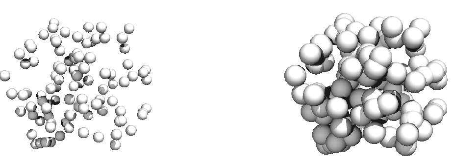
Obviously, this transition must occur much earlier (at a small $r_{c}$) when the distribution is not homogeneous in three dimensions. We do not fully implement this method of Minkowski functionals [9], but next neighbor distances obviously do yield significant information.

The code of about 100 lines given below reproduces the results given in section 3. It can easily be run with different data sets and future data releases of SDSS. We plan to add some refinements for a second version, but also the reader should be able to do slight modifications or extensions of the code. A quick description for getting started is found in section 5.1. Though we cannot give a detailed description of the program, some clarifying comments are included in the quite self-explaining code (see  5.2).

2 Methods

2.1 General method and limitations

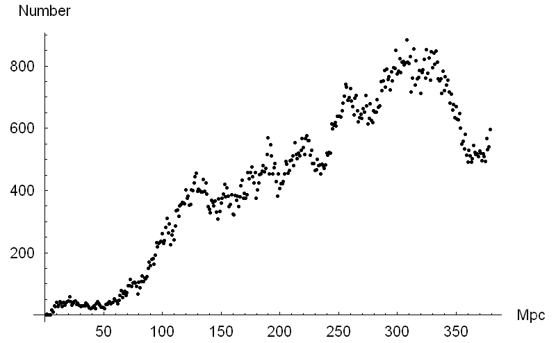
As a first approximative approach, we did not take into consideration galaxy size and morphology, which may well influence a more refined analysis. Spectra were just used to determine the distance by the redshift, $H_{0}$ was assumed as $72\ kms^{-1}Mpc^{-1}$ [10, 11]. Though peculiar velocities cause errors in the radial distance, no correction was tried so far to take into account that effect. To avoid faint galaxies to drop out of the sample, we considered redshifts $z<0.03$, the point to which the SDSS data show a roughly constant density. There is a clearly visible decay of the number of galaxies per volume for $D>130\ Mpc$ or $z>0.03$ (see fig. 2).

Figure 2: Galaxy number between $D$ and $D+dD$ as a function of distance $D$. Constant density should lead to a parabolic increase of the number of galaxies with distance. For $D>130\ Mpc$ or $z>0.03$, obviously a considerable percentage of galaxies are too faint to be detected.

2.2 Data acquisition

Figure 3: Coverage of spectral data from SDSS DR6 site

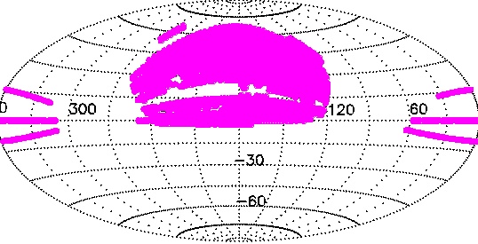
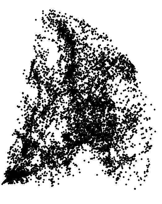
The sixth data release (DR6) of the SDSS data is located in $http://www.sdss.org/dr6$ (see fig. 3). Though very simple data sets can be accessed by search masks, we strongly recommend the use of SQL data search language to which the SDSS site provides very good tutorials. The part of the sky taken into consideration was determined by the SDSS coverage. We chose $140^{\circ}<DEC240^{\circ}$ and $30^{\circ}<RA60^{\circ}$ and a second sample $140^{\circ}<DEC240^{\circ}$ and $-2^{\circ}<RA11^{\circ}$. See fig. 4 for a 3D-plot of the galaxies of sample 1. The confidence level was set to $0.35$. The respective SQL commands for downloading the data are listed in the appendix 5.1.

Figure 4: 3D-plot of the position of the 9280 galaxies of sample 1.

2.3 Data manipulation and modelling

We used the computer algebra system $Mathematica$ to convert the raw data to Euclidean coordinates. Thus the distances to the next neighbor could be calculated easily. Then, these minimal or next neighbor distances for each galaxy contain the desired structure information. For a large number of $i$ points, an effective minimal distance algorithm is needed, since computing all distances would lead to an increase of computational time $t\sim i^{2}$. We chose a very simple method that leads to $t\sim i$. The entire volume was divided by a rectangular lattice in $n^{3}$ boxes of equal size, e.g. for $n=10$ into 1000 boxes. In a first step, each galaxy was assigned to its box. To determine the minimal distance of an individual galaxy, the computation of all distances within one box and the 26 neighboring boxes was sufficient. Likewise, the random distributions were analyzed, whereby in the 2D-case a $n^{2}$-lattice with larger $n$ was chosen. The 3D- simulation consisted of a cube with the same volume as the real sample shown in fig. (4). The galaxy density was equal to the real one. For the 2D-simulation, the size of the surface of a sphere was chosen, while the spherical volume was equal to the real one. Due to computational simplicity, the form of the surface was a square.

3 Results - a preliminary analysis

Figure 5: Sorted next-neighbor-distances, for the real distribution (black) and the simulations in 3-D (dark gray) and 2D (light gray). Sample from the region $60^{\circ}>DEC>30^{\circ}$ and $240^{\circ}>RA>140^{\circ}$.

Figure 6: as fig. 5, but for a smaller sample $11^{\circ}>DEC>-2^{\circ}$ and $240^{\circ}>RA>140^{\circ}$.

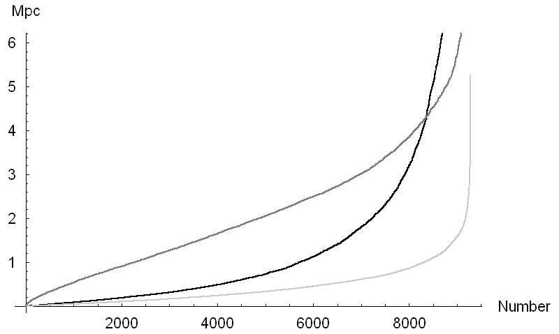
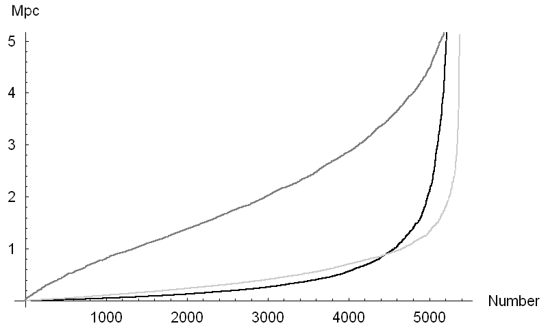
The real sorted distances (fig. 5 and 6) exclude clearly a homogeneous 3D-distribution which would lead to greatly different next-neighbor-distances. They also coincide well with the 2D random distribution on a surface, as far as small distances are concerned. The approach to the 3D-simulation for larger distances could indicate a homogeneity of the universe on larger scales. We do not know how peculiar velocities influence, the effect should however be limited to $D<5\ Mpc$ ([4], p. 6) Next neighbors which occasionally are to faint to be detected could as well spoil the analysis at larger distances. Especially the presence of large voids in the real distribution may explain why there the largest next-neighbor-distances exceed those of the random distribution. Therefore, as mentioned in the introduction, an interpretation of the present data in favor of a large-scale homogenity instead of a fractal dimension $D=2$ would be premature. We have no explanation so far for the difference visible in the two samples fig. (5) and (6).

4 Conclusions

The distribution of galaxies in the universe is still a riddle and theoretically not fully understood [5]. The discovery of the two-dimensional structure of the galaxy distribution reminds us from something deep and mysterious, such as from Dirac’s observation of a twodimensional density in the universe. Particulary $\Lambda$CDM simulations have problems to account for the observed structure. Observational progress in this field is therefore very much triggered by new high-quality data like SDSS. The ongoing discussion can thus benefit from a broad accessibility of those data and a transparent processing which is not limited to a few groups. If one day the data allow a definite answer to decide whether the large scale structure is homogeneous of even fractal, this must become evident also for the non-expert scientist. We hope this is a little step towards repeatability and transparency for the efforts to answer that important question.

Acknowledgement.

Though we are grateful for any comments, please understand that we cannot guarantee functionality or give further support for getting this program to run on your computer.

5 Appendix: data preparation and source code

5.1 Step-by step procedure in 10 minutes

1. Create your directory ‘sdss’ and copy all the following files in there.

2. Browse to $http://www.alexander-unzicker.de/sdss1.txt$ and copy the file. Alternatively, copy and paste from the arXiv source and save as $sdss1.txt$.

3. Browse to $http://cas.sdss.org/dr6/en/tools/search/sql.asp$

4. Type the following SQL commands in the blank field (you may paste and copy it also from the end of the $sdss1.txt$ file):

select ra,dec,z
from specObj
where ra BETWEEN 140 and 240 AND
dec BETWEEN 30 and 60 AND
specClass = 2 AND
z BETWEEN 0.001 AND 0.03
AND zConf > 0.35

1. Chose file format CSV.

2. Press submit and save the data file as $sdss03.csv$.

3. Proceed likewise for dec between -2 and 11 and save as $sdss03a.csv$.

4. Open a Mathematica *.nb file and run the following commands (apart from the SetDirectory comand where you have to put in your path, you may paste and copy it also from the end of the $sdss1.txt$ file)

SetDirectory["yoursdsspath"];
<<"sdss1.txt";
readData["sdss03.csv"];  (* later sdss03a.csv *)
GalPlot[{100, 500, 700}];
fastDistances[rpt, xyz, {20, 20, 20}, {rarg, decrg, rrg}];
randomDistances3d[vol^(1/3), Galnumber, {20, 20, 20}];
randomDistances2d[(3 vol/4/Pi)^(1/3) Sqrt[4 Pi], Galnumber, {90, 90}];
compareDistances[0.004]; (** creates one plot from 3  ***)

5.2 Source code

<<Statistics‘DataManipulation‘;
(************** plot options *************)
sty2={{GrayLevel[0.3],Thickness[0.01]},{GrayLevel[0.5],
Thickness[0.01]},{GrayLevel[0.8],Thickness[0.01]}};
(********************* constants ************************)
cc=299792458; H0=1/(4.4081 10^(17)); Mpc=3.08567758128*10^(22);(*corresponds to 70 km/s/Mpc*)
offset = 0.00000001;(**** to avoid division by zero ****)
(************* functions needed ************************)
tor[z_]:=(2cc z+cc z^2)/(H0 Mpc(2+2z+z^2));(* transformation from redshift to Mpc distance *)
toxyz[{r_,th_,ph_}]:={r Sin[th]Cos[ph],r Sin[th]Sin[ph],r Cos[th]}; (*to cartesian coord.*)
dist2[k1_,k2_]:=Apply[Plus, (k1-k2)^2];(*square of distance of two points k1, k2 in 3 dim.*)
(*************** procedures**********************************)
(********* reads SDSS data in *.csv format  *****************)
readData[infile_]:=Block[{qwe,wer,wer1,ra,dec,rr, zz}, (* local variables *)
If[FileInformation[infile]=={},Print["file not found."]; Goto[endlabel]]; (* check infile *)
qwe = Drop[Import[infile, "CSV"], 1]; wer1 = Transpose[qwe];
wer = ReplacePart[wer1, offset, Position[wer1, 0]];(* replace undesired zeros *)
ra = 2 Pi wer[[1]]/360; dec=2 Pi wer[[2]]/360; zz=wer[[3]]; (* angle in radians *)
(*** automatic boundary determination from data , ranges of coordinates ****)
{ramin, decmin}={Min[ra]-offset,Min[dec]-offset};
{ramax, decmax}={Max[ra]+offset,Max[dec]+offset};
zmin=Min[zz]-offset; zmax=Max[zz]+offset; rarg=ramax-ramin; decrg=decmax-decmin;
zrg=zmax-zmin; meandec=(decmax+decmin)/2;
rrmax = tor[zmax]; rrmin = tor[zmin]; rrg = rrmax - rrmin;
rr = Map[tor, zz]; (*** transformation redshift - radius**)
rpt=Transpose[{rr, dec, ra}]; (*spherical coordinates*)
xyz= Map[toxyz, rpt];(* transform to cartesian coordinates *)
vol=(rrmax^3-rrmin^3) 4/3 Pi rarg/(2Pi) decrg/(2Pi) Abs[Cos[meandec]];(* mind latitude *)
Galnumber=Length[rpt]; GalDichte=Galnumber/vol;
Print["Number of galaxies: ", Galnumber]; Print["Volume in Mpc^3: ", vol];
Label[endlabel]];
(************** calculates real distances *************************)
realDistances[rpt_,xyz_,unt_,rgs_]:=Block[{}, tu1=TimeUsed[];
{rarg, decrg, rrg}=rgs; (* ranges*)
box = mindist = Table[{}, {unt[[1]]}, {unt[[2]]}, {unt[[3]]}];
(* empty variable for the boxes and minimal distances*)
(* assign each galaxy to its box *)
(* though boxes are defined by polar coordinates, they contain cartesian ones *)
For[i = 1, i <= Galnumber, i++, AppendTo[box[[Ceiling[(rpt[[i, 1]] - rrmin)/rrg *unt[[1]]],
   Ceiling[(rpt[[i, 2]]-decmin)/decrg*unt[[2]]],
   Ceiling[(rpt[[i,3]]-ramin)/rarg *unt[[3]]]]],xyz[[i]]]];
tu2=TimeUsed[];Print["assign to boxes... ",tu2-tu1, "s"];
(**** distance in box i,j,k to all other galaxies in the box and in neighboring boxes ******)
For[i = 1, i <= unt[[1]], i++,
  For[j = 1, j <= unt[[2]], j++,
    For[k = 1, k <= unt[[3]], k++,
        For[m = 1, m <= Length[box[[i, j, k]]], m++, distances={};
          (*now go through neighboring boxes ii,jj, kk *)
  For[ii = i-1, ii <=i+1, ii++,
    For[jj = j-1, jj <= j+1, jj++,
      For[kk = k-1, kk <= k+1, kk++,
        If[(ii==0 || jj==0 || kk==0 || ii==unt[[1]]+1 || jj==unt[[2]]+1 || kk==unt[[3]]+1),
            Continue,
   If[box[[ii,jj,kk]]!={},AppendTo[distances,Table[dist2[box[[i,j,k,m]],box[[ii,jj,kk,mm]]],
      {mm,Length[box[[ii, jj, kk]]]}]]]]; ]]];  (* avoid pathologic cases like empty boxes *)
         If[(distances!={} && Flatten[distances]!={0.}),
            AppendTo[mindist[[i,j,k]],Sort[Flatten[distances]][[2]]]];
]]]];
tu1=TimeUsed[];Print["measuring...",tu1-tu2, "s"];
distToNext = Flatten[mindist]; rowOfDist=Sort[distToNext];
ListPlot[rowOfDist,PlotJoined ->True, AxesLabel -> {"Number", "Mpc"}]];
(******* calculates distances of random distibutions in 3D  *****************)
randomDistances3d[edge_,nn_,unt_]:=
Block[{box,mindist,distances,distToNext, i,j,k,m}, tu1=TimeUsed[];
xyz=Table[edge{Random[],Random[],Random[]},{i,nn}];
box = mindist = Table[{}, {unt[[1]]}, {unt[[2]]}, {unt[[3]]}];
(* empty variable for the boxes and minimal distances*)
(* assign each galaxy to its box *)
For[i = 1, i <= nn, i++, AppendTo[box[[Ceiling[(xyz[[i, 1]])/edge*unt[[1]]],
 Ceiling[(xyz[[i, 2]])/edge*unt[[2]]], Ceiling[(xyz[[i,3]])/edge*unt[[3]]]]], xyz[[i]]]];
tu2=TimeUsed[];Print["assign to boxes...  ",tu2-tu1, "s"];
For[i = 1, i <= unt[[1]], i++,
   For[j = 1, j <= unt[[2]], j++,
     For[k = 1, k <= unt[[3]], k++,
         For[m = 1, m <= Length[box[[i, j, k]]], m++, distances={};
         (*now go through neighboring boxes ii,jj, kk *)
 For[ii = i-1, ii <=i+1, ii++,
    For[jj = j-1, jj <= j+1, jj++,
      For[kk = k-1, kk <= k+1, kk++,
        If[(ii==0 || jj==0 || kk==0 || ii==unt[[1]]+1 || jj==unt[[2]]+1 || kk==unt[[3]]+1),
           Continue,
             If[box[[ii,jj,kk]]!={},AppendTo[distances, Table[dist2[box[[i,j,k,m]],
                 box[[ii,jj,kk,mm]]],{mm,Length[box[[ii, jj, kk]]]}]]]];
            ]]];
            If[(distances!={}&& Flatten[distances]!={0.}),
               AppendTo[mindist[[i,j,k]],Sort[Flatten[distances]][[2]]]];
]]]];
tu1=TimeUsed[];Print["measuring...",tu1-tu2, "s"];
distToNext = Flatten[mindist];
rowOfDist3=Sort[distToNext];
ListPlot[rowOfDist3,PlotJoined ->True, AxesLabel -> {"Number", "Mpc"}]];
(******* calculates distances of random distibutions in 2D  *****************)
randomDistances2d[edge_,nn_,unt_]:=
Block[{box,mindist,distances,distToNext, i,j,m}, tu1=TimeUsed[];
xy=Table[edge{Random[],Random[]},{i,nn}];
box = mindist = Table[{}, {unt[[1]]}, {unt[[2]]}];
(* empty variable for the boxes and minimal distances*)
(* assign each galaxy to its box *)
For[i = 1, i <= nn, i++, AppendTo[box[[Ceiling[(xy[[i, 1]])/edge*unt[[1]]],
 Ceiling[(xy[[i, 2]])/edge*unt[[2]]]]], xy[[i]]]];
tu2=TimeUsed[];Print["assign to boxes...  ",tu2-tu1, "s"];
For[i = 1, i <= unt[[1]], i++,
  For[j = 1, j <= unt[[2]], j++,
     For[m = 1, m <= Length[box[[i, j]]], m++, distances={};
          (*now go through neighboring boxes ii,jj *)
 For[ii = i-1, ii <=i+1, ii++,
   For[jj = j-1, jj <=j+1, jj++,
      If[(ii==0 || jj==0 || ii==unt[[1]]+1 || jj==unt[[2]]+1), Continue,
      If[box[[ii,jj]]!={},AppendTo[distances, Table[dist2[box[[i,j,m]],
           box[[ii,jj,mm]]],{mm,Length[box[[ii, jj]]]}]]]];
       ]];
        If[(distances!={}&& Flatten[distances]!={0.}),
            AppendTo[mindist[[i,j]],Sort[Flatten[distances]][[2]]]];
]]];
tu1=TimeUsed[];Print["measuring...",tu1-tu2, "s"];
distToNext = Flatten[mindist];
rowOfDist2=Sort[distToNext];
ListPlot[rowOfDist2,PlotJoined ->True, AxesLabel -> {"Number", "Mpc"}]];
(***************** plot of galaxy distribution **************************)
GalPlot[vp_(*chose appropriate ViewPoint*)]:=Show[Graphics3D[Map[Point, xyz]],
Boxed->False, ViewPoint -> vp, Prolog->AbsolutePointSize[0.0005]];
compareDistances[th_]:=Block[{},$DefaultFont={"Arial", 8};
lp1 = ListPlot[rowOfDist, PlotStyle -> {Thickness[th],GrayLevel[0]},
PlotJoined->True, DisplayFunction -> Identity];
lp2 = ListPlot[rowOfDist2, PlotStyle ->{Thickness[th],GrayLevel[0.8]},
PlotJoined->True,  DisplayFunction -> Identity];
lp3 = ListPlot[rowOfDist3, PlotStyle -> {Thickness[th],GrayLevel[0.5]},
PlotJoined->True,   DisplayFunction -> Identity];
distrib=Show[lp1,lp2,lp3, DisplayFunction -> $DisplayFunction,
AspectRatio -> .6, AxesLabel -> {"Number", "Mpc"}]];

References

- [1] V. de Lapparent, M. J. Geller, and J. P. Huchra. A slice of the universe. Astrophysical Journal Letters, 302:L1–L5, March 1986.
- [2] M. J. Geller and J. P. Huchra. Mapping the universe. Science, 246:897–903, November 1989.
- [3] J. R. Gott, III, M. Dickinson, and A. L. Melott. The sponge-like topology of large-scale structure in the universe. Astrophysical Journal, 306:341–357, July 1986.
- [4] F.Sylos Labini, N.L. Vasilyev, L. Pietronero, and Y.V. Baryshev. The large scale inhomogeneity of the galaxy distribution. ArXiv.org:0805.1132, 2008.
- [5] P. J. E. Peebles. The Void Phenomenon. Astrophysical Journal, 2001, astro-ph/0101127.
- [6] J. R. I. Gott, D. C. Hambrick, M. S. Vogeley, J. Kim, C. Park, Y.-Y. Choi, R. Cen, J. P. Ostriker, and K. Nagamine. Genus Topology of Structure in the Sloan Digital Sky Survey: Model Testing. Astrophysical Journal, 2008, astro-ph/0610762.
- [7] A. Unzicker and D. Schmidle. A quick and dirty approach to verify the Pioneer anomaly. arXiv, gr-qc/0702151, 2007.
- [8] M. Ostermann. Unpublished manuscript from sfb 375. 2007.
- [9] K. R. Mecke, T. Buchert, and H. Wagner. Robust morphological measures for large-scale structure in the Universe. Astronomy and Astrophysics, 288:697–704, 1994, astro-ph/9312028.
- [10] A.G. Riess et. al. Cepheid Calibrations from the Hubble Space Telescope of the Luminosity of Two Recent Type Ia Supernovae and a Re-determination of the Hubble Constant. The Astrophysical Journal, 627:579, 2005, astro-ph/0503159.
- [11] Neal Jackson. The Hubble Constant. LIVING REVIEWS IN RELATIVITY, 10:4, 2007, arxiv: 0709.3924.